From the free course CS323: Numerical Analysis and Computing on Lykke
Numerical Linear Algebra: Vectors, Matrices, and Norms
Key concepts: Vector and Matrix Algebra · Vector Operations · Linear Independence · Column Space & Null Space · Vector Norms (L1, L2, L-infinity) · Matrix Norms · Condition Number
This section reviews the fundamental building blocks of numerical linear algebra. It covers the definitions and operations of vectors and matrices, key theoretical concepts like span and column space, and the crucial idea of norms for measuring the magnitude of vectors and matrices. Understanding norms is essential for analyzing error and the sensitivity of linear systems.
Numerical Linear Algebra: Vectors, Matrices, and Norms
In most real-world applications, from simulating fluid dynamics to training a deep neural network, we rarely operate on single numbers. Instead, numerical computation is performed on entire collections of numbers. Vector and matrix algebra provides the fundamental mathematical framework for organizing, manipulating, and analyzing this data. This section provides a deep dive into the essential tools of this framework: vectors, matrices, and the concept of a norm, which allows us to measure the 'size' or 'magnitude' of these objects. This ability to quantify size is the bedrock for analyzing the error, stability, and convergence of nearly all numerical algorithms.
Vectors: The Building Blocks
At its core, linear algebra is the study of vectors and the linear transformations that act upon them. Vectors are the fundamental objects, representing points in space, quantities with direction, or simply ordered lists of data.
Definition and Notation
A vector in
n-dimensional real space, denotedv ∈ ℝⁿ, is an orderedn-tuple of real numbers.v = (v₁, v₂, ..., vₙ)
By convention in numerical linear algebra, a vector is treated as a column vector, which is an n × 1 matrix:
v = \begin{pmatrix} v_1 \\ v_2 \\ \vdots \\ v_n \end{pmatrix}
Its transpose, vᵀ, is a row vector, which is a 1 × n matrix: vᵀ = $$ \begin{pmatrix} v_1 & v_2 & \dots & v_n \end{pmatrix} $$ . This distinction is not merely pedantic; it becomes critical when performing matrix operations. The space ℝⁿ is the set of all such n-dimensional vectors.
Fundamental Vector Operations
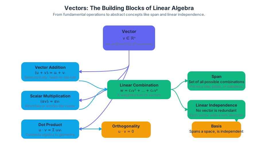
The power of vectors comes from the algebraic structure defined on ℝⁿ. The two primary operations are vector addition and scalar multiplication.
-
Vector Addition: If
u, v ∈ ℝⁿ, their sumu + vis defined by component-wise addition:(u + v)ᵢ = uᵢ + vᵢ. Geometrically, this corresponds to the "head-to-tail" rule, forming a parallelogram. -
Scalar Multiplication: If
v ∈ ℝⁿandα ∈ ℝis a scalar, their productαvis defined by multiplying each component ofvbyα:(αv)ᵢ = αvᵢ. Geometrically, this scales the vector, stretching or shrinking it and possibly reversing its direction ifα < 0.
These two operations together allow us to form linear combinations.
- Dot Product (Inner Product): The dot product of two vectors
u, v ∈ ℝⁿis a scalar value defined as:u ⋅ v = uᵀv = Σᵢ uᵢvᵢ.
The dot product is immensely useful as it connects algebra to geometry. It can be used to find the length of a vector and the angle between two vectors. The geometric definition of the dot product is u ⋅ v = ||u|| ||v|| cos(θ), where θ is the angle between u and v. This shows that two non-zero vectors are orthogonal (perpendicular) if and only if their dot product is zero.
Concrete Example: Vector Operations in Code
While high-level libraries provide optimized routines, implementing these operations from scratch reveals their underlying mechanics.
import numpy as np
import math

def manual_dot_product(v1: np.ndarray, v2: np.ndarray) -> float:
    """
    Computes the dot product of two 1D NumPy arrays without using np.dot or @.
    This demonstrates the fundamental summation algorithm.
    """
    if v1.shape != v2.shape or v1.ndim != 1:
        raise ValueError("Vectors must be 1D and have the same shape.")

    dot_product_sum = 0.0
    for i in range(v1.shape[0]):
        dot_product_sum += v1[i] * v2[i]
    return dot_product_sum

# --- Example Usage ---
u = np.array([1.0, -2.0, 3.0])
v = np.array([4.0, 5.0, 6.0])

# Scalar multiplication and vector addition
w = 2 * u + v
print(f"Vector u = {u}")
print(f"Vector v = {v}")
print(f"Result of 2*u + v = {w}\n")

# Dot product comparison
manual_result = manual_dot_product(u, v)
numpy_result = np.dot(u, v)
operator_result = u @ v # Python 3.5+ infix operator for matrix multiplication

print(f"Manual dot product: {manual_result}")
print(f"NumPy's np.dot result: {numpy_result}")
print(f"Using @ operator: {operator_result}\n")

# Geometric application: finding the angle between u and v
# cos(theta) = (u . v) / (||u|| ||v||)
norm_u = math.sqrt(manual_dot_product(u, u))
norm_v = math.sqrt(manual_dot_product(v, v))
cos_theta = manual_result / (norm_u * norm_v)
angle_rad = math.acos(cos_theta)
angle_deg = math.degrees(angle_rad)

print(f"Norm of u: {norm_u:.4f}")
print(f"Norm of v: {norm_v:.4f}")
print(f"Angle between u and v: {angle_deg:.2f} degrees")
Linear Combinations, Span, and Linear Independence
These concepts form the theoretical foundation of vector spaces.
-
A linear combination of a set of vectors
{v¹, v², ..., vᵏ}is any vectorwthat can be written asw = c₁v¹ + c₂v² + ... + cₖvᵏ, wherecᵢare scalar coefficients. -
The span of a set of vectors is the set of all possible linear combinations of those vectors. The span of a set of vectors in
ℝⁿforms a subspace ofℝⁿ(e.g., a line or a plane passing through the origin). -
A set of vectors
{v¹, v², ..., vᵏ}is linearly independent if the only solution to the equationc₁v¹ + c₂v² + ... + cₖvᵏ = 0isc₁ = c₂ = ... = cₖ = 0. Intuitively, this means no vector in the set can be expressed as a linear combination of the others. They each contribute a unique, non-redundant direction. If a set is not linearly independent, it is linearly dependent.
Why it matters: Linear independence is a cornerstone concept. In solving systems of equations, it tells us whether a solution is unique. In data science, it relates to multicollinearity, where features are redundant. A set of n linearly independent vectors in ℝⁿ forms a basis for that space, meaning any vector in ℝⁿ can be uniquely represented as a linear combination of these basis vectors.
Matrices: Linear Transformations Encapsulated
A matrix can be viewed in several ways: as a grid of numbers, a collection of vectors, or, most powerfully, as an object that represents a linear transformation between vector spaces.
Definition and Notation
An
m × nmatrixAis a rectangular array of numbers withmrows andncolumns. We writeA ∈ ℝ^(m×n). The entry in thei-th row andj-th column is denotedAᵢⱼoraᵢⱼ.
A = \begin{pmatrix}
A_{11} & A_{12} & \dots & A_{1n} \\
A_{21} & A_{22} & \dots & A_{2n} \\
\vdots & \vdots & \ddots & \vdots \\
A_{m1} & A_{m2} & \dots & A_{mn}
\end{pmatrix}
Matrix-Vector Multiplication
The product of an m × n matrix A and an n × 1 vector x results in an m × 1 vector y. This operation, y = Ax, is the engine of linear algebra and has two fundamental interpretations.
Interpretation 1: Row-wise (Dot Products) Each component
yᵢof the output vectoryis the dot product of thei-th row ofAwith the vectorx.
yᵢ = Aᵢ,₁x₁ + Aᵢ,₂x₂ + ... + Aᵢ,ₙxₙ = Σⱼ Aᵢⱼxⱼ
Interpretation 2: Column-wise (Linear Combination) The output vector
yis a linear combination of the columns ofA, where the coefficients are the components ofx.
y = x₁A₁,: + x₂A₂,: + ... + xₙAₙ,:
The column-wise view is often more insightful. It reveals that the output Ax must lie within the span of the columns of A.
// Let A be an m x n matrix and x be an n x 1 vector.
// The product y = Ax is an m x 1 vector.

// Interpretation 1: Dot products with rows
y_i = \sum_{j=1}^{n} A_{ij} x_j \quad \text{for } i=1, \ldots, m

// Example for y_1:
y_1 = (A_{1,1} * x_1) + (A_{1,2} * x_2) + \dots + (A_{1,n} * x_n)

// Interpretation 2: Linear combination of columns
// Let A_{:,j} be the j-th column of A.
y = x_1 A_{:,1} + x_2 A_{:,2} + \dots + x_n A_{:,n}

// Example:
\begin{pmatrix} y_1 \\ \vdots \\ y_m \end{pmatrix} = x_1 \begin{pmatrix} A_{1,1} \\ \vdots \\ A_{m,1} \end{pmatrix} + x_2 \begin{pmatrix} A_{1,2} \\ \vdots \\ A_{m,2} \end{pmatrix} + \dots + x_n \begin{pmatrix} A_{1,n} \\ \vdots \\ A_{m,n} \end{pmatrix}
Column Space & Null Space
These two subspaces are intrinsically linked to any matrix A ∈ ℝ^(m×n) and are critical for understanding the behavior of the linear system Ax = b.
-
Column Space
C(A): The column space ofAis the span of its column vectors. It is a subspace of the output spaceℝᵐ.- What it is: The set of all possible output vectors
bfor which the systemAx = bhas a solution. - Why it matters: If a vector
bis not inC(A), thenAx = bis inconsistent and has no solution. The dimension ofC(A)is the rank of the matrix,rank(A) = r.
- What it is: The set of all possible output vectors
-
Null Space
N(A): The null space ofAis the set of all input vectorsxthat are mapped to the zero vector. It is a subspace of the input spaceℝⁿ.- What it is: The set of all solutions to the homogeneous equation
Ax = 0. - Why it matters: The null space tells us about the uniqueness of solutions. If
N(A)contains only the zero vector, then the solution toAx = b(if it exists) is unique. IfN(A)is non-trivial, there are infinitely many solutions. The dimension ofN(A)is the nullity of the matrix.
- What it is: The set of all solutions to the homogeneous equation
These two spaces are part of the Four Fundamental Subspaces of linear algebra, which provide a complete geometric picture of a linear transformation.
| Subspace | Definition | Resides in | Dimension | Interpretation |
|---|---|---|---|---|
Column Space C(A) |
Span of columns of A |
ℝᵐ |
r (rank) |
All possible outputs b for Ax=b |
Null Space N(A) |
All x such that Ax=0 |
ℝⁿ |
n-r |
Solutions to the homogeneous equation |
Row Space C(Aᵀ) |
Span of rows of A |
ℝⁿ |
r (rank) |
Orthogonal complement of N(A) |
Left Null Space N(Aᵀ) |
All y such that Aᵀy=0 |
ℝᵐ |
m-r |
Orthogonal complement of C(A) |
This structure leads to a profound result: the Rank-Nullity Theorem.
Theorem (Rank-Nullity): For any matrix
A ∈ ℝ^(m×n), the dimension of its column space (rank) plus the dimension of its null space (nullity) equals the number of columnsn.
rank(A) + nullity(A) = n
This theorem provides a beautiful accounting of dimensions. It states that the number of dimensions in the input space (n) is split between the dimensions that are preserved and mapped to the output space (rank) and the dimensions that are collapsed to zero (nullity).
Vector Norms: Measuring Magnitude
In numerical analysis, we constantly need to quantify the size of vectors, especially error vectors. A norm is a function that generalizes the concept of "length" or "magnitude" to vector spaces.
Formal Definition of a Norm
A function ||.|| : ℝⁿ → ℝ is a vector norm if for any vectors x, y ∈ ℝⁿ and any scalar α ∈ ℝ, it satisfies:
- Non-negativity:
||x|| ≥ 0, and||x|| = 0if and only ifx = 0. - Absolute Scalability (Homogeneity):
||αx|| = |α| ||x||. - Triangle Inequality:
||x + y|| ≤ ||x|| + ||y||.
The triangle inequality is the most important property. It formalizes the idea that the shortest path between two points is a straight line.
The p-Norms: A Family of Measures
A broad and useful family of norms are the p-norms (or Lp-norms), defined as:
||x||_p = (Σᵢ |xᵢ|^p)^(1/p) for p ≥ 1.
The three most common instances of p-norms are essential tools in scientific computing and machine learning.
-
L1 Norm (
p=1, Manhattan Norm):||x||₁ = Σᵢ |xᵢ|.- How it works: It sums the absolute values of the components. It's called the "Manhattan norm" because it represents the distance a taxi would travel on a grid of streets.
- Why it matters: The L1 norm is widely used in machine learning (e.g., Lasso regression) because it promotes sparsity. Minimizing the L1 norm of a vector of parameters tends to drive many of the parameters to exactly zero, effectively performing feature selection.
-
L2 Norm (
p=2, Euclidean Norm):||x||₂ = sqrt(Σᵢ xᵢ²).- How it works: This is the standard geometric length of a vector, calculated via the Pythagorean theorem. It is the square root of the dot product of a vector with itself:
||x||₂ = sqrt(xᵀx). - Why it matters: It is the most natural measure of distance. It is used everywhere, from calculating residuals in least-squares problems to regularization in Ridge regression. Unlike the L1 norm, it is differentiable everywhere (except at the origin), which is a convenient property for optimization algorithms.
- How it works: This is the standard geometric length of a vector, calculated via the Pythagorean theorem. It is the square root of the dot product of a vector with itself:
-
L-infinity Norm (
p→∞, Max Norm):||x||_∞ = maxᵢ |xᵢ|.- How it works: It is simply the largest absolute value among the components of the vector.
- Why it matters: The L-infinity norm is used when we care about the worst-case error. It isolates the component with the maximum magnitude, which is often crucial in error analysis and ensuring stability.
Geometric Interpretation and Use Cases
The "unit ball" for each norm (the set of all vectors x such that ||x|| ≤ 1) reveals their geometric character.
| Norm | Formula | Geometric Shape (Unit Ball in ℝ²) | Common Use Case |
|---|---|---|---|
| L1 Norm (` | x | ||
| L2 Norm (` | x | ||
| L-infinity Norm (` | x |
Real-World Usage: Gradient Clipping in Deep Learning
In training deep neural networks, gradients can sometimes become excessively large, leading to unstable training. A common technique to prevent this is gradient clipping, which uses a norm to rescale gradients if their magnitude exceeds a threshold.
import torch

# Imagine this is a gradient tensor for a layer's weights during backpropagation
gradients = torch.tensor([-2.5, 0.8, 1.2, -4.0, 0.1])

# Calculate different norms of the gradient vector
l1_norm = torch.linalg.vector_norm(gradients, ord=1)
l2_norm = torch.linalg.vector_norm(gradients, ord=2)
linf_norm = torch.linalg.vector_norm(gradients, ord=float('inf'))

print(f"Gradient Tensor: {gradients}")
print(f"L1 Norm (Sum of absolute values): {l1_norm:.4f}")
print(f"L2 Norm (Euclidean length): {l2_norm:.4f}")
print(f"L-infinity Norm (Max absolute value): {linf_norm:.4f}")

# A common use case: Gradient Clipping by L2 norm
# If the L2 norm of the gradients exceeds a threshold, scale it down.
max_norm_threshold = 2.0
if l2_norm > max_norm_threshold:
    clip_coefficient = max_norm_threshold / l2_norm
    clipped_gradients = gradients * clip_coefficient

    print(f"\nL2 norm ({l2_norm:.2f}) exceeded threshold {max_norm_threshold}. Gradients clipped.")
    print(f"Clipped Gradients: {clipped_gradients}")
    print(f"New L2 Norm: {torch.linalg.vector_norm(clipped_gradients, ord=2):.4f}")
Matrix Norms: Quantifying Amplification
Just as we need to measure the size of vectors, we also need to measure the "size" or "strength" of matrices. A matrix norm quantifies the maximum effect a matrix can have on a vector.
Induced (or Operator) Norms
The most natural way to define a matrix norm is by its action on vectors. An induced norm measures the maximum "stretching factor" that the matrix applies to any vector, as measured by a specific vector norm.
The matrix norm
||A||induced by a vector norm||.||is defined as:||A|| = sup_{x≠0} (||Ax|| / ||x||) = sup_{||x||=1} ||Ax||
This definition means the matrix norm is the largest possible value of the ratio ||Ax|| / ||x||. It answers the question: "What is the maximum amplification this matrix can produce?"
Each vector p-norm induces a corresponding matrix p-norm.
- Matrix 1-Norm:
||A||₁ = max_j Σᵢ |Aᵢⱼ|(Maximum absolute column sum). - Matrix ∞-Norm:
||A||_∞ = max_i Σⱼ |Aᵢⱼ|(Maximum absolute row sum). - Matrix 2-Norm (Spectral Norm):
||A||₂ = σ_max(A), whereσ_maxis the largest singular value ofA. This norm corresponds to the true maximum stretching factor but is the most computationally expensive to calculate.
The Frobenius Norm: An Alternative View
Not all matrix norms are induced. The Frobenius norm is a commonly used alternative that is easier to compute. It treats the matrix as if it were a single long vector and calculates its L2 norm.
The Frobenius norm of a matrix
A ∈ ℝ^(m×n)is defined as:||A||_F = sqrt(Σᵢ Σⱼ Aᵢⱼ²) = sqrt(tr(AᵀA))
Pitfall: While the Frobenius norm is a valid matrix norm (it satisfies the three defining properties), it is not an induced norm. It does not represent the maximum amplification factor in the same way ||A||₂ does. However, its computational simplicity makes it popular for applications like low-rank matrix approximation.
| Norm | Type | Formula | Computational Cost |
|---|---|---|---|
| Matrix 1-Norm (` | A | ||
| Matrix ∞-Norm (` | A | ||
| Matrix 2-Norm (` | A | ||
| Frobenius Norm (` | A |
Example: Calculating Matrix Norms from the Command Line
We can use command-line tools like Octave/MATLAB for quick calculations, demonstrating another environment where these concepts are applied.
# Using octave-cli for a quick, interactive calculation of various norms for a matrix.
# This shows how these concepts are built into numerical computing environments.

# Define a 2x2 matrix A = [[1, -7], [-2, -3]]
octave-cli --eval "A = [1, -7; -2, -3]; \
                   norm_1 = norm(A, 1); \
                   norm_inf = norm(A, inf); \
                   norm_2 = norm(A, 2); \
                   norm_fro = norm(A, 'fro'); \
                   printf('Matrix A:\n'); disp(A); \
                   printf('1-Norm (max col sum of |1|+|-2|=3 and |-7|+|-3|=10): %f\n', norm_1); \
                   printf('Inf-Norm (max row sum of |1|+|-7|=8 and |-2|+|-3|=5): %f\n', norm_inf); \
                   printf('2-Norm (spectral norm, max singular value): %f\n', norm_2); \
                   printf('Frobenius Norm (sqrt(1^2 + (-7)^2 + (-2)^2 + (-3)^2)): %f\n', norm_fro);"
Output:
Matrix A:
   1  -7
  -2  -3

1-Norm (max col sum of |1|+|-2|=3 and |-7|+|-3|=10): 10.000000
Inf-Norm (max row sum of |1|+|-7|=8 and |-2|+|-3|=5): 8.000000
2-Norm (spectral norm, max singular value): 7.333245
Frobenius Norm (sqrt(1^2 + (-7)^2 + (-2)^2 + (-3)^2)): 7.937254
This example clearly shows that different norms give different measures of the "size" of the same matrix, each with its own interpretation and use case. The concepts of norms are the foundation for the condition number of a matrix, which is one of the most critical quantities in numerical analysis for determining the stability and reliability of a solution to a linear system.
Source Materials
Study CS323: Numerical Analysis and Computing on Lykke
This course page is free to open: signed out, you can read its first two sections, and signing in, on any plan, opens the rest. The free Lykke Chrome extension syncs your own Canvas courses, so ChatGPT, Claude and Muse can answer from your classes and deadlines. It only reads Canvas.
Add the free extensionSign in to open every sectionAll sections of CS323: Numerical Analysis and Computing · Browse more course pages