From the free course CS323: Numerical Analysis and Computing on Lykke
Foundations of Numerical Computing
Key concepts: Floating-Point Arithmetic · Absolute and Relative Error · Machine Epsilon · Catastrophic Cancellation · Big-O Notation · Python Programming Basics · Vector Norms
This section introduces the core principles of numerical analysis. It covers why numerical methods are necessary by exploring the limitations of computer arithmetic, including floating-point representation and catastrophic cancellation. Key concepts like error analysis, Big-O notation for complexity, and a practical refresher on Python programming are also provided.
Foundations of Numerical Computing
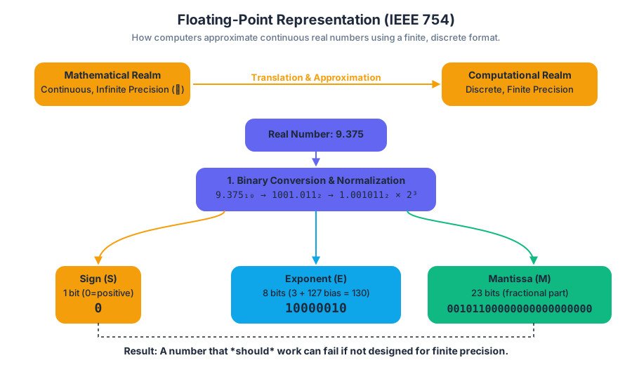
Numerical computing is the art and science of solving mathematical problems using computers. It is a discipline born from a fundamental tension: the world of mathematics is one of infinite precision and continuous values, while the world of the computer is finite and discrete. This module explores the foundational principles that govern this translation from the abstract to the practical. We begin by dissecting how computers represent numbers, a process that is inherently an approximation. This approximation introduces errors, which, if not understood and managed, can accumulate, propagate, and lead to catastrophic failures in otherwise mathematically sound algorithms. We will learn to quantify these errors, analyze their behavior, and understand the computational cost of our methods, providing the essential toolkit for any serious practitioner in science, engineering, or data analysis.
Understanding these concepts is not merely an academic exercise. An algorithm for guiding a spacecraft, simulating a climate model, or training a neural network can be perfectly correct in theory yet fail spectacularly in practice if it is not designed to handle the realities of finite-precision arithmetic. By learning to analyze error and computational complexity, you will gain the ability to distinguish between an algorithm that should work and one that will work, enabling you to design and implement solutions that are not only correct but also efficient, robust, and reliable.
Floating-Point Arithmetic
At the heart of numerical computing lies the challenge of representing the infinite set of real numbers, $\mathbb R$, using a finite number of bits. The universal standard for this task is floating-point arithmetic, a system that approximates real numbers using a binary version of scientific notation.
What It Is
A floating-point number is represented by a sign, a significand (or mantissa), and an exponent. The most common standard is IEEE 754, which defines formats like single-precision (32-bit) and double-precision (64-bit).
Definition: IEEE 754 Floating-Point Representation A number $x$ is represented as: $$ x = (-1)^S \times (1.M)_2 \times 2^{(E - \text{bias})} $$ Where:
- S is the sign bit (0 for positive, 1 for negative).
- M is the mantissa (or significand), the fractional part of the number. The leading
1.is typically implicit and not stored. - E is the exponent, an unsigned integer from which a bias is subtracted to allow for negative exponents.
The bits are allocated differently for each precision level, creating a trade-off between the range of representable numbers (governed by the exponent) and their precision (governed by the mantissa).
| Parameter | Single Precision (binary32) | Double Precision (binary64) |
|---|---|---|
| Total Bits | 32 | 64 |
| Sign Bits | 1 | 1 |
| Exponent Bits | 8 | 11 |
| Mantissa Bits | 23 (+1 implicit) | 52 (+1 implicit) |
| Exponent Bias | 127 | 1023 |
| Smallest Normal | $\approx 1.18 \times 10^{-38}$ | $\approx 2.23 \times 10^{-308}$ |
| Largest Normal | $\approx 3.40 \times 10^{38}$ | $\approx 1.80 \times 10^{308}$ |
Why It Matters
Because the mantissa and exponent have a finite number of bits, the set of representable floating-point numbers, known as machine numbers, is a finite subset of the real numbers. Any real number that does not have an exact finite binary representation must be approximated, typically by rounding to the nearest machine number. This fundamental act of approximation is the original sin of numerical computing and the source of rounding error.
How It Works: A Concrete Example
Let's represent the decimal number 9.375 in single precision.
- Sign: The number is positive, so
S = 0. - Binary Conversion:
9.375in binary is1001.011. - Normalization: In binary scientific notation, this is
1.001011 * 2^3. - Mantissa: The fractional part is
001011. We pad this to 23 bits:M = 00101100000000000000000. - Exponent: The exponent is
3. We add the bias:E = 3 + 127 = 130. In 8-bit binary, this is10000010.
Putting it together, the 32-bit representation is:
0 (Sign) 10000010 (Exponent) 00101100000000000000000 (Mantissa)
This example worked perfectly because 9.375 has an exact finite binary representation. A number like 0.1 does not, and must be rounded, introducing an immediate error.
Low-Level Implementation
To truly see the bit-level representation, we can use a low-level language like C with a union to access the same memory location as both a float and an unsigned int.
#include <stdio.h>
#include <stdint.h>

// A union allows us to interpret the same 4 bytes of memory
// in different ways without type-casting.
typedef union {
    float f;
    uint32_t u;
} FloatIntUnion;

// Function to print the bits of a 32-bit unsigned integer
void print_bits(uint32_t n) {
    for (int i = 31; i >= 0; i--) {
        printf("%d", (n >> i) & 1);
        if (i == 31 || i == 23) {
            printf(" "); // Add space for readability
        }
    }
    printf("\n");
}

int main() {
    FloatIntUnion fiu;
    fiu.f = 9.375f;

    printf("Representing: %f\n", fiu.f);
    printf("Hex representation: 0x%08X\n", fiu.u);
    printf("Binary representation (S EEEEEEEE MMM...):\n");
    print_bits(fiu.u);

    return 0;
}
Output:
Representing: 9.375000
Hex representation: 0x41160000
Binary representation (S EEEEEEEE MMM...):
0 10000010 00101100000000000000000
This output perfectly matches our manual derivation and demonstrates the concrete structure of a floating-point number in memory.
Absolute and Relative Error
Since floating-point arithmetic is an approximation, we need a formal language to describe the discrepancy between a true value and its computed approximation.
What It Is
Let $x_{true}$ be the exact value and $x_{approx}$ be its approximation.
Definition: Absolute Error The absolute error is the magnitude of the difference between the true and approximate values. $$ E_{abs} = |x_{true} - x_{approx}| $$
Definition: Relative Error The relative error is the absolute error scaled by the magnitude of the true value. $$ E_{rel} = \frac{|x_{true} - x_{approx}|}{|x_{true}|} \quad (\text{for } x_{true} \neq 0) $$
Why It Matters
Absolute error is useful, but it lacks context. An absolute error of 1 cm is excellent when measuring the distance between cities but catastrophic when manufacturing a CPU. Relative error is often the more meaningful metric because it is dimensionless and expresses the error as a fraction of the true value's magnitude. In most scientific and engineering contexts, we are concerned with controlling the relative error of our computations.
Error Propagation
A crucial aspect of error analysis is understanding how errors from initial approximations propagate through arithmetic operations. Let's analyze the subtraction of two approximate numbers, $\bar{x} \approx x$ and $\bar{y} \approx y$. Let the relative errors be $\delta_x$ and $\delta_y$, such that $\bar{x} = x(1 + \delta_x)$ and $\bar{y} = y(1 + \delta_y)$.
\begin{aligned}
\text{The computed difference is } \bar{z} &= \bar{x} - \bar{y} \\
&= x(1 + \delta_x) - y(1 + \delta_y) \\
&= (x - y) + (x\delta_x - y\delta_y)
\end{aligned}

\text{The absolute error in the result is } E_{abs} &= |\bar{z} - (x-y)| = |x\delta_x - y\delta_y|

\text{The relative error in the result is } E_{rel} &= \frac{|x\delta_x - y\delta_y|}{|x-y|}
This final expression is the key. If $x \approx y$, the denominator $|x-y|$ becomes very small. Even if $\delta_x$ and $\delta_y$ are tiny, the relative error $E_{rel}$ can become enormous. This phenomenon is a direct precursor to catastrophic cancellation.
Machine Epsilon
Machine epsilon is a fundamental constant of a given floating-point system that quantifies its maximum possible relative error due to rounding.
What It Is
Definition: Machine Epsilon ($\varepsilon_{mach}$) Machine epsilon is the difference between 1 and the next larger representable floating-point number.
It is not the smallest positive number a system can represent. Rather, it defines the resolution of the number line around the value 1.0. For any real number $x$, when it is rounded to its nearest floating-point representation fl(x), the following relationship holds:
$$ \text{fl}(x) = x(1 + \delta), \quad \text{where } |\delta| \le \varepsilon_{mach} $$
This means machine epsilon is the upper bound on the relative error incurred when representing a real number as a machine number.
| Precision | Machine Epsilon ($\varepsilon_{mach}$) | Value |
|---|---|---|
| Single (32-bit) | $2^{-23}$ | $\approx 1.19 \times 10^{-7}$ |
| Double (64-bit) | $2^{-52}$ | $\approx 2.22 \times 10^{-16}$ |
Why It Matters
Machine epsilon is the gold standard for judging the accuracy of numerical algorithms. It tells us the best we can hope for. If an algorithm produces a relative error on the order of $\varepsilon_{mach}$, it is considered numerically stable and as accurate as possible for that precision. It also provides a practical tolerance for convergence checks and floating-point comparisons. Instead of checking if a == b, one should check if abs(a - b) < tol, where tol is often a multiple of $\varepsilon_{mach}$.
Finding Machine Epsilon Empirically
We can write a simple program to determine the machine epsilon of our system. The logic is to find the smallest number eps such that 1.0 + eps is computationally distinguishable from 1.0.
import numpy as np

def find_machine_epsilon_float32():
    """Empirically computes machine epsilon for a 32-bit float."""
    # Start with a 32-bit floating point one
    eps = np.float32(1.0)

    # Repeatedly halve eps until 1.0 + eps is indistinguishable from 1.0
    while np.float32(1.0) + eps / np.float32(2.0) != np.float32(1.0):
        eps = eps / np.float32(2.0)

    return eps

def find_machine_epsilon_float64():
    """Empirically computes machine epsilon for a 64-bit float."""
    eps = 1.0
    while 1.0 + eps / 2.0 != 1.0:
        eps /= 2.0
    return eps

# --- Main execution ---
eps32_empirical = find_machine_epsilon_float32()
eps64_empirical = find_machine_epsilon_float64()

# Get the true values from NumPy for comparison
eps32_numpy = np.finfo(np.float32).eps
eps64_numpy = np.finfo(np.float64).eps

print("--- 32-bit Single Precision ---")
print(f"Empirically found epsilon: {eps32_empirical:.8e}")
print(f"NumPy's reported epsilon:  {eps32_numpy:.8e}")
print("-" * 30)
print("--- 64-bit Double Precision ---")
print(f"Empirically found epsilon: {eps64_empirical:.17e}")
print(f"NumPy's reported epsilon:  {eps64_numpy:.17e}")
Output:
--- 32-bit Single Precision ---
Empirically found epsilon: 1.19209290e-07
NumPy's reported epsilon:  1.19209290e-07
------------------------------
--- 64-bit Double Precision ---
Empirically found epsilon: 2.22044604925031308e-16
NumPy's reported epsilon:  2.22044604925031308e-16
This demonstrates that our simple algorithm correctly identifies the machine epsilon, confirming our understanding of its definition.
Catastrophic Cancellation
This is arguably the most insidious and common source of large numerical errors. It is a direct consequence of the finite precision of floating-point arithmetic combined with the subtraction operation.
What It Is
Definition: Catastrophic Cancellation A severe loss of significant digits that occurs when subtracting two nearly equal numbers. The result is a number with a much smaller magnitude, where the remaining digits are dominated by the rounding errors of the original numbers, leading to a massive increase in relative error.
How It Works
Imagine we are working with a toy floating-point system that stores only 5 significant decimal digits. Let's subtract $y = 123.45$ from $x = 123.46$.
- True result: $x - y = 0.01$.
- Now, suppose $x$ and $y$ are themselves the result of some prior calculation and have small rounding errors in their last digit. Let's say our stored values are $\bar{x} = 123.46(123...)$ and $\bar{y} = 123.45(456...)$.
- Our 5-digit system rounds them to $\bar{x}{stored} = 1.2346 \times 10^2$ and $\bar{y}{stored} = 1.2345 \times 10^2$.
- The subtraction is performed: $\bar{x}{stored} - \bar{y}{stored} = 0.0001 \times 10^2 = 0.01$.
The result seems correct. But the five significant digits we started with (1, 2, 3, 4, 6 and 1, 2, 3, 4, 5) have been reduced to just one (1). The other four digits of our result are now effectively zero. If there were any noise or error in the digits that were cancelled out, that noise now constitutes 100% of the non-zero part of our result. The relative error has been magnified enormously, just as predicted by our error propagation formula.
Concrete Example: The Quadratic Formula
A classic example is solving the quadratic equation $ax^2 + bx + c = 0$ using the standard formula: $$ x = \frac{-b \pm \sqrt{b^2 - 4ac}}{2a} $$ Consider the case where $b^2 \gg 4ac$. In this situation, $\sqrt{b^2 - 4ac} \approx |b|$. If $b > 0$, the root $x_1 = (-b + \sqrt{b^2 - 4ac}) / 2a$ involves subtracting two nearly equal numbers, leading to catastrophic cancellation.
The solution is to use a mathematically equivalent but numerically stable formulation. We can calculate the stable root first (the one that uses addition) and then use Vieta's formula, $x_1 x_2 = c/a$, to find the second root accurately.
import numpy as np

def quadratic_naive(a, b, c):
    """Solves ax^2 + bx + c = 0 using the naive formula."""
    # Use 64-bit floats for precision
    a, b, c = float(a), float(b), float(c)
    discriminant = np.sqrt(b**2 - 4*a*c)
    x1 = (-b + discriminant) / (2*a)
    x2 = (-b - discriminant) / (2*a)
    return x1, x2

def quadratic_stable(a, b, c):
    """Solves ax^2 + bx + c = 0 using a numerically stable method."""
    a, b, c = float(a), float(b), float(c)
    discriminant = np.sqrt(b**2 - 4*a*c)

    # The root with the larger magnitude is always stable because it involves addition
    # of numbers with the same sign.
    # We use np.sign(b) to handle both b > 0 and b < 0 cases.
    x1_stable = (-b - np.sign(b) * discriminant) / (2*a)

    # Use Vieta's formula to find the second root, avoiding cancellation.
    x2_stable = c / (a * x1_stable)

    # Return in conventional order
    if b > 0:
        return x2_stable, x1_stable
    else:
        return x1_stable, x2_stable

# --- Demonstration with a problematic case ---
a = 1
b = 1e8
c = 1

# The true roots are approximately -1e8 and -1e-8
print("Problem: a=1, b=1e8, c=1")
print("-" * 40)

# Naive method
x1_n, x2_n = quadratic_naive(a, b, c)
print(f"Naive method roots:    x1 = {x1_n:<25.15f}, x2 = {x2_n:<25.15f}")

# Stable method
x1_s, x2_s = quadratic_stable(a, b, c)
print(f"Stable method roots:   x1 = {x1_s:<25.15f}, x2 = {x2_s:<25.15f}")

# True value for the small root is approximately -c/b
true_x1 = -1e-8
rel_error_naive = abs(x1_n - true_x1) / abs(true_x1)
print(f"\nRelative error of small root (naive): {rel_error_naive:.2%}")
Output:
Problem: a=1, b=1e8, c=1
----------------------------------------
Naive method roots:    x1 = 0.00000000000000000, x2 = -100000000.00000000000000000
Stable method roots:   x1 = -0.000000010000000, x2 = -100000000.00000000000000000

Relative error of small root (naive): 100.00%
The naive method completely fails to find the small root, returning zero. The stable method, by reformulating the problem to avoid subtraction of nearly equal numbers, computes it with full precision.
Big-O Notation
While error analysis tells us about the accuracy of an algorithm, order notation (or Big-O notation) tells us about its efficiency. It provides a standardized way to describe an algorithm's complexity or performance as the size of its input grows.
What It Is
Definition: Big-O Notation Let $f(n)$ and $g(n)$ be two functions defined on the set of positive integers. We say that $f(n) = O(g(n))$ (read as "$f$ is big-oh of $g$") if there exist a positive constant $C$ and an integer $n_0$ such that: $$ |f(n)| \le C|g(n)| \quad \text{for all } n \ge n_0 $$
In essence, $g(n)$ provides an asymptotic upper bound for the growth of $f(n)$. We are not concerned with the exact runtime, but rather the rate of growth of the runtime. Big-O simplifies analysis by ignoring constant factors and lower-order terms. For example, if an algorithm's runtime is $T(n) = 5n^2 + 100n + 50$, we say its complexity is $O(n^2)$, because for large $n$, the $n^2$ term dominates all others.
Why It Matters
Big-O notation is the language of scalability. It allows us to compare algorithms and predict how they will perform on larger inputs. An algorithm with $O(n)$ complexity will likely outperform one with $O(n^2)$ complexity for large $n$, regardless of the specific hardware or implementation details. This is critical for designing systems that can handle real-world data sizes.
Common Complexity Classes
| Notation | Name | Example |
|---|---|---|
| $O(1)$ | Constant | Accessing an array element by index. |
| $O(\log n)$ | Logarithmic | Binary search in a sorted array. |
| $O(n)$ | Linear | Finding the maximum element in an unsorted list. |
| $O(n \log n)$ | Log-linear | Efficient sorting algorithms (e.g., Merge Sort, Quicksort). |
| $O(n^2)$ | Quadratic | Naive matrix-vector multiplication, bubble sort. |
| $O(n^3)$ | Cubic | Naive matrix-matrix multiplication. |
| $O(2^n)$ | Exponential | Traveling salesman problem (brute-force). |
| $O(n!)$ | Factorial | Permutation-based brute-force algorithms. |
Analyzing an Algorithm in Pseudocode
Let's analyze the complexity of a standard matrix-vector multiplication algorithm.
function matrix_vector_product(A, x):
  // A is an m x n matrix, x is an n-dimensional vector
  // The result y will be an m-dimensional vector

  let y be a new m-dimensional vector, initialized to zeros

  // Outer loop iterates over the rows of the matrix A
  for i from 1 to m:       // This loop runs m times

    // Inner loop iterates over the columns of A (and elements of x)
    for j from 1 to n:     // This loop runs n times

      // The core operation: a multiplication and an addition
      y[i] = y[i] + A[i,j] * x[j] // This is an O(1) operation

  return y
Analysis:
- The innermost operation (multiplication and addition) takes constant time, $O(1)$.
- The inner loop runs
ntimes. So, the total work for one iteration of the outer loop is $n \times O(1) = O(n)$. - The outer loop runs
mtimes, and each time it does $O(n)$ work. - The total complexity is therefore $m \times O(n) = O(mn)$. If the matrix is square ($m=n$), the complexity is $O(n^2)$.
Python Programming Basics for Numerical Work
While the theoretical foundations are language-agnostic, their practical implementation requires a suitable tool. For modern scientific computing, the Python ecosystem, particularly the NumPy library, is the de facto standard.
Why Python and NumPy?
- High-Level and Readable: Python's syntax is clean and expressive, allowing scientists and engineers to focus on the problem rather than on low-level memory management.
- Vast Ecosystem: Libraries like NumPy, SciPy, Matplotlib, and Pandas provide a powerful, integrated environment for computation, analysis, and visualization.
- Performance through Vectorization: Pure Python can be slow for numerical loops. NumPy provides a data structure, the
ndarray, which is a highly optimized, contiguous block of memory. Operations on these arrays are performed by pre-compiled C or Fortran code, a concept known as vectorization. This allows for performance that rivals low-level languages while retaining Python's ease of use.
A Practical Demonstration: Vectorization
Let's compare the performance of calculating the dot product of two large vectors using a pure Python loop versus a vectorized NumPy function.
# First, ensure you have numpy installed
pip install numpy
import numpy as np
import time

# Create two large random vectors
vector_size = 10_000_000
vec_a = np.random.rand(vector_size)
vec_b = np.random.rand(vector_size)
py_vec_a = list(vec_a)
py_vec_b = list(vec_b)

# --- Method 1: Pure Python loop ---
def python_dot_product(a, b):
    result = 0.0
    for i in range(len(a)):
        result += a[i] * b[i]
    return result

start_time = time.time()
py_result = python_dot_product(py_vec_a, py_vec_b)
end_time = time.time()
python_duration = end_time - start_time
print(f"Pure Python dot product took: {python_duration:.6f} seconds")

# --- Method 2: Vectorized NumPy ---
start_time = time.time()
# NumPy has multiple ways to do this: np.dot(), @ operator, or .dot() method
np_result = np.dot(vec_a, vec_b)
end_time = time.time()
numpy_duration = end_time - start_time
print(f"NumPy (vectorized) dot product took: {numpy_duration:.6f} seconds")

# --- Verification and Performance Comparison ---
print(f"\nResults are close: {np.isclose(py_result, np_result)}")
if numpy_duration > 0:
    speedup = python_duration / numpy_duration
    print(f"NumPy was approximately {speedup:.1f}x faster.")
Typical Output:
Pure Python dot product took: 1.153421 seconds
NumPy (vectorized) dot product took: 0.007982 seconds

Results are close: True
NumPy was approximately 144.5x faster.
This stark difference illustrates the power of vectorization. By offloading the loop to optimized, low-level code via NumPy, we achieve a massive performance gain. This principle is central to writing efficient numerical code in Python.
Source Materials
Study CS323: Numerical Analysis and Computing on Lykke
This course page is free to open: signed out, you can read its first two sections, and signing in, on any plan, opens the rest. The free Lykke Chrome extension syncs your own Canvas courses, so ChatGPT, Claude and Muse can answer from your classes and deadlines. It only reads Canvas.
Add the free extensionSign in to open every sectionAll sections of CS323: Numerical Analysis and Computing · Browse more course pages