From the free course Calculus I: Single Variable Calculus on Lykke
Part 3: Coordinate Systems & Infinite Series
Key concepts: Coordinate Systems · Infinite Series · Convergence and Divergence · Taylor Series
Examines advanced topics including polar coordinates and the convergence of infinite sequences and series.
Part 3: Coordinate Systems & Infinite Series
The transition from the calculus of functions in Cartesian space to the study of infinite series and alternative coordinate systems represents a fundamental shift in mathematical maturity. In the previous sections, we focused on the local behavior of functions (derivatives) and the accumulation of quantities (integrals). In Part 3, we address the approximation of reality. As Professor Gigliola Staffilani emphasizes in MIT’s 18.01 curriculum, the goal is to bridge the gap between abstract notation and intuitive physical meaning. Whether we are describing the spiral path of a particle in a magnetic field or approximating a transcendental function for a microprocessor, the tools of coordinate transformation and series expansion are indispensable.
Coordinate Systems: Beyond the Grid
While the Cartesian (rectangular) coordinate system is the bedrock of Euclidean geometry, it is often the most difficult system to use when describing natural phenomena. Circular motion, planetary orbits, and wave propagation often possess radial symmetry that makes $x$ and $y$ coordinates cumbersome.
Polar Coordinates
In a Polar Coordinate System, a point $P$ in the plane is determined by a distance $r$ from a fixed point $O$ (the pole/origin) and an angle $\theta$ from a fixed ray (the polar axis).
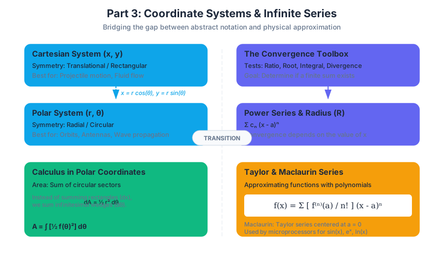
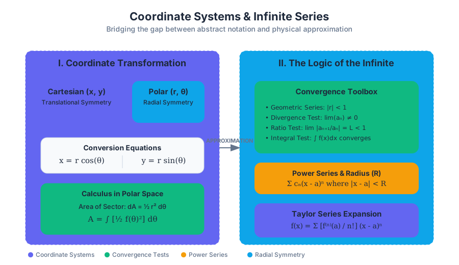
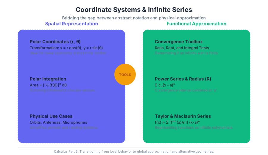
Definition: The relationship between Cartesian coordinates $(x, y)$ and Polar coordinates $(r, \theta)$ is defined by the transformation equations: $$x = r \cos(\theta)$$ $$y = r \sin(\theta)$$ Where $r^2 = x^2 + y^2$ and $\tan(\theta) = y/x$.
Why Polar Coordinates Matter
In engineering and physics, polar coordinates simplify the equations of motion for rotating systems. For instance, the equation of a circle with radius $a$ centered at the origin is the complex $x^2 + y^2 = a^2$ in Cartesian terms, but simply $r = a$ in polar terms.
| Feature | Cartesian $(x, y)$ | Polar $(r, \theta)$ |
|---|---|---|
| Symmetry | Translational / Rectangular | Radial / Circular |
| Grid Lines | Straight lines ($x=c, y=c$) | Concentric circles ($r=c$), Rays ($\theta=c$) |
| Best Use Case | Projectile motion, Fluid flow in pipes | Orbits, Microphones (Polar patterns), Antennas |
| Complexity | High for curves (square roots) | Low for periodic/circular functions |
Calculus in Polar Coordinates: Area and Arc Length
To find the area $A$ of a region bounded by a polar curve $r = f(\theta)$, we do not use rectangles. Instead, we sum the areas of infinitesimal circular sectors.
The area of a sector is given by $dA = \frac{1}{2}r^2 d\theta$. Thus, the total area is: $$A = \int_{\alpha}^{\beta} \frac{1}{2} [f(\theta)]^2 d\theta$$
Infinite Series: The Logic of the Infinite
An Infinite Series is the sum of the terms of an infinite sequence. The central question of series calculus is not "What is the sum?" but rather "Does the sum exist?" (Convergence vs. Divergence).
Convergence and Divergence
A series $\sum_{n=1}^{\infty} a_n$ converges to a sum $S$ if the sequence of its partial sums $S_k = \sum_{n=1}^{k} a_n$ approaches $S$ as $k \to \infty$. If the partial sums do not approach a finite limit, the series diverges.
The Convergence Toolbox
Determining convergence requires a suite of tests. Choosing the right test is a matter of pattern recognition.
| Test Name | Condition for Convergence | Common Use Case |
|---|---|---|
| Geometric Series | $\vert r\vert < 1$ for $\sum ar^n$ | Fractal geometry, Zeno's paradox |
| Divergence Test | If $\lim_{n \to \infty} a_n \neq 0$, it diverges | Quick first check for any series |
| Integral Test | $\int_{1}^{\infty} f(x) dx$ converges | $p$-series, logarithmic series |
| Ratio Test | $\lim_{n \to \infty} \vert \frac{a_{n+1}}{a_n}\vert < 1$ | Power series, factorials, exponentials |
| Root Test | $\lim_{n \to \infty} \sqrt[n]{\vert a_n\vert } < 1$ | Terms raised to the $n$-th power |
The Ratio Test: The Engineer's Favorite
The Ratio Test is arguably the most powerful tool for power series. It measures the "growth rate" of terms. If the terms shrink fast enough (faster than a geometric series), the sum is finite.
\text{Given } \sum a_n, \text{ calculate } L = \lim_{n \to \infty} \left| \frac{a_{n+1}}{a_n} \right|
\begin{cases}
L < 1 & \text{Absolutely Convergent} \\
L > 1 & \text{Divergent} \\
L = 1 & \text{Inconclusive (Try Integral Test)}
\end{cases}
Power Series and the Radius of Convergence
A Power Series is a series of the form: $$\sum_{n=0}^{\infty} c_n (x - a)^n = c_0 + c_1(x-a) + c_2(x-a)^2 + \dots$$ This is essentially an "infinite polynomial" centered at $a$. Unlike a standard series, a power series may converge for some values of $x$ and diverge for others.
The Radius of Convergence ($R$)
Every power series has a Radius of Convergence $R$.
- The series converges only when $x = a$ ($R=0$).
- The series converges for all $x$ ($R=\infty$).
- The series converges for $|x - a| < R$ and diverges for $|x - a| > R$.
The behavior at the endpoints ($x = a-R$ and $x = a+R$) must be checked separately using other convergence tests.
Taylor and Maclaurin Series
The pinnacle of single-variable calculus is the Taylor Series. It allows us to represent any infinitely differentiable function as a power series. This is how calculators compute $\sin(1.5)$ or $\ln(2)$; they don't look up a table, they calculate a polynomial approximation.
The General Formula
The Taylor series for a function $f(x)$ centered at $a$ is: $$f(x) = \sum_{n=0}^{\infty} \frac{f^{(n)}(a)}{n!} (x - a)^n$$ If $a=0$, the series is specifically called a Maclaurin Series.
Theorem (Taylor’s Theorem): If $f(x)$ is approximated by its $n$-th degree Taylor polynomial $P_n(x)$, the remainder (error) $R_n(x) = f(x) - P_n(x)$ is given by: $$R_n(x) = \frac{f^{(n+1)}(c)}{(n+1)!} (x - a)^{n+1}$$ for some $c$ between $a$ and $x$. This allows us to bound the error of our approximation.
Common Maclaurin Series
These series are the "building blocks" of mathematical analysis.
| Function | Series Expansion | Interval of Convergence |
|---|---|---|
| $e^x$ | $1 + x + \frac{x^2}{2!} + \frac{x^3}{3!} + \dots$ | $(-\infty, \infty)$ |
| $\sin x$ | $x - \frac{x^3}{3!} + \frac{x^5}{5!} - \dots$ | $(-\infty, \infty)$ |
| $\cos x$ | $1 - \frac{x^2}{2!} + \frac{x^4}{4!} - \dots$ | $(-\infty, \infty)$ |
| $\frac{1}{1-x}$ | $1 + x + x^2 + x^3 + \dots$ | $(-1, 1)$ |
Real-World Application: Small Angle Approximation
In physics and structural engineering, Taylor series are used to simplify differential equations. For small oscillations (like a pendulum), we use the first term of the Taylor series for $\sin \theta$: $$\sin \theta \approx \theta$$ This turns a non-linear differential equation into a linear one, which is solvable by hand. This "linearization" is the foundation of control theory and stability analysis.
Common Pitfalls and Misconceptions
- Ignoring the Interval of Convergence: A common mistake is using a Taylor series outside its radius of convergence. For example, the series for $\ln(1+x)$ only converges for $-1 < x \leq 1$. Trying to calculate $\ln(5)$ using this series directly will result in divergence.
- Confusing Sequences and Series: A sequence is a list ($a_1, a_2, \dots$); a series is a sum ($a_1 + a_2 + \dots$). A sequence can converge to zero while its series diverges (e.g., the Harmonic Series $\sum 1/n$).
- Polar Coordinate Ambiguity: Unlike Cartesian coordinates, polar coordinates are not unique. The point $(1, \pi)$ is the same as $(-1, 0)$ and $(1, 3\pi)$. This "multi-valued" nature can lead to errors when setting integration limits.
- The "Divergence Test" Fallacy: If $\lim a_n = 0$, the series might converge. It is not a guarantee. The Harmonic Series is the classic counter-example.
Pedagogical Insight: Visualizing the Abstract
Professor Staffilani’s approach to these topics emphasizes that "math is not just symbols on a page." When teaching polar coordinates, she often uses physical props—like a balloon being inflated—to show how radial growth ($dr$) relates to the surface area. For infinite series, she bridges the gap by relating them to digital signals: every digital audio file is essentially a series of approximations (Fourier Series, a relative of Taylor Series) that our ears perceive as continuous sound.
By moving from the rigid grid of Descartes to the fluid rotations of Polar space, and from the exactness of closed-form functions to the flexible power of infinite series, we gain the ability to model the complex, the non-linear, and the infinite.
Source Materials
Study Calculus I: Single Variable Calculus on Lykke
This course page is free to open: signed out, you can read its first two sections, and signing in, on any plan, opens the rest. The free Lykke Chrome extension syncs your own Canvas courses, so ChatGPT, Claude and Muse can answer from your classes and deadlines. It only reads Canvas.
Add the free extensionSign in to open every sectionAll sections of Calculus I: Single Variable Calculus · Browse more course pages