From the free course Calculus I: Single Variable Calculus on Lykke
Part 2: Integration
Key concepts: Integration · Fundamental Theorem of Calculus · Accumulation Functions · Area Under a Curve
Covers the principles of integration, focusing on accumulation and the area under curves.
Part 2: Integration
Integration is often introduced as the "inverse" of differentiation, but this characterization, while technically true, undersells its profound conceptual depth. If differentiation is the study of local change—the "instantaneous" snapshot of a system—then integration is the study of accumulation. It is the mathematical machinery that allows us to reconstruct the whole from its infinitesimal parts.
In the pedagogical tradition of MIT’s 18.01, as championed by Professor Gigliola Staffilani, integration is not merely a set of algorithmic procedures (like the Power Rule in reverse). Instead, it is approached as a bridge between the abstract and the tangible. By using visual tools, physical props, and digital applets, we move from the "black box" of the integral symbol $\int$ to a deep understanding of how quantities like area, volume, work, and probability are built from the ground up.
The Definite Integral: The Geometry of Accumulation
The formal journey into integration begins with the Area Problem: how do we calculate the area under a curve $f(x)$ between two points $a$ and $b$? While Euclidean geometry gives us formulas for squares and circles, it fails for the arbitrary, fluctuating curves of the real world.
The Riemann Sum
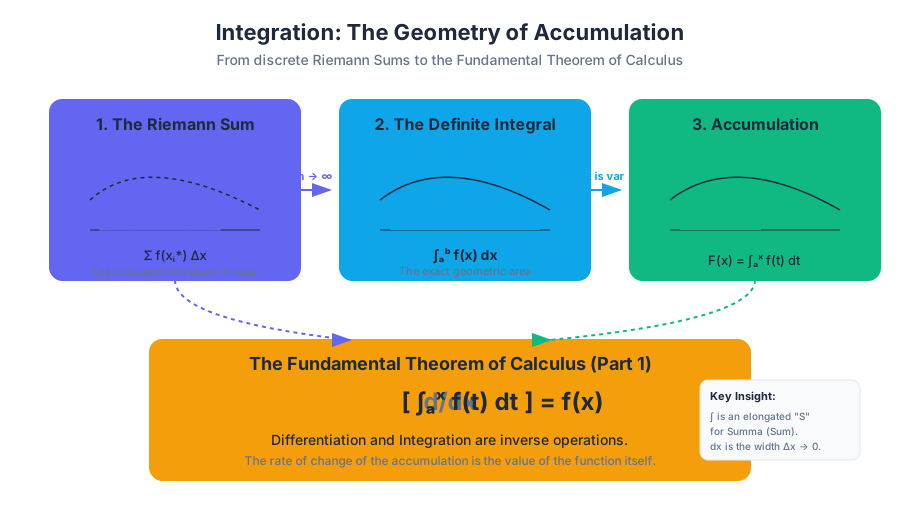
The solution lies in the Riemann Sum. We partition the interval $[a, b]$ into $n$ sub-intervals of width $\Delta x = \frac{b-a}{n}$. Within each sub-interval, we pick a sample point $x_i^$ and construct a rectangle with height $f(x_i^)$. The total area is approximated by the sum of these rectangles:
$$S_n = \sum_{i=1}^{n} f(x_i^*) \Delta x$$
As $n \to \infty$ (and $\Delta x \to 0$), this sum converges to the Definite Integral:
$$\int_{a}^{b} f(x) , dx = \lim_{n \to \infty} \sum_{i=1}^{n} f(x_i^*) \Delta x$$
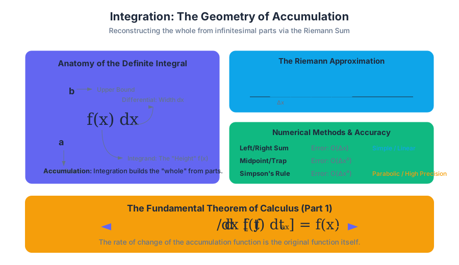
Key Insight: The $dx$ in the integral notation is not just a decorative tag; it represents the infinitesimal width of the rectangles, while $f(x)$ represents the height. The integral sign $\int$ is an elongated "S," standing for summa (sum).
Comparison of Approximation Methods
Depending on where we choose $x_i^*$ (the sample point), the accuracy of our finite sum varies significantly.
| Method | Selection of $x_i^*$ | Error Characteristic | Best Use Case |
|---|---|---|---|
| Left Riemann Sum | Left endpoint of sub-interval | $O(\Delta x)$; Overestimates if $f$ is decreasing | Quick manual approximations |
| Right Riemann Sum | Right endpoint of sub-interval | $O(\Delta x)$; Overestimates if $f$ is increasing | Theoretical proofs |
| Midpoint Rule | Center of sub-interval | $O(\Delta x^2)$; Much more accurate than L/R | General numerical integration |
| Trapezoidal Rule | Average of endpoints | $O(\Delta x^2)$; Connects points with lines | Data sets with discrete points |
| Simpson's Rule | Parabolic fit over two intervals | $O(\Delta x^4)$; Extremely high precision | Scientific computing / Engineering |
The Accumulation Function
Before we can link integration to differentiation, we must understand the Accumulation Function, denoted as $F(x)$.
$$F(x) = \int_{a}^{x} f(t) , dt$$
The Dummy Variable
A common point of confusion for students is the introduction of $t$. In the expression above, $x$ is the independent variable of $F$, defining the right-hand boundary of the area. $t$ is a dummy variable—a placeholder that "sweeps" across the interval $[a, x]$.
Physical Intuition
Think of $f(t)$ as the rate of water flowing into a tank (liters per second). $F(x)$ is the total volume of water in the tank at time $x$. If the flow rate $f(t)$ is high, the volume $F(x)$ increases rapidly. If $f(t)$ is zero, the volume $F(x)$ stays constant.
The Fundamental Theorem of Calculus (FTC)
The FTC is the "Great Unification" of calculus. It bridges the gap between the geometry of areas (integration) and the physics of motion (differentiation). It consists of two parts.
FTC Part 1: The Derivative of an Integral
FTC Part 1 states that if $f$ is continuous, then the accumulation function $F(x)$ is the antiderivative of $f(x)$.
$$\frac{d}{dx} \left[ \int_{a}^{x} f(t) , dt \right] = f(x)$$
This tells us that differentiation and integration are inverse operations. If you accumulate a rate of change and then look at the rate at which that accumulation is growing, you get back to the original rate.
Derivation of FTC Part 1
We use the limit definition of the derivative on the accumulation function $F(x)$:
\begin{aligned}
F'(x) &= \lim_{h \to 0} \frac{F(x+h) - F(x)}{h} \\
&= \lim_{h \to 0} \frac{1}{h} \left[ \int_{a}^{x+h} f(t)dt - \int_{a}^{x} f(t)dt \right] \\
&= \lim_{h \to 0} \frac{1}{h} \int_{x}^{x+h} f(t)dt
\end{aligned}
By the Mean Value Theorem for Integrals, there exists a $c$ in $[x, x+h]$ such that $\int_{x}^{x+h} f(t)dt = f(c) \cdot h$. Substituting this in:
$$F'(x) = \lim_{h \to 0} \frac{f(c) \cdot h}{h} = \lim_{h \to 0} f(c)$$
As $h \to 0$, $c$ is forced to $x$. Since $f$ is continuous, $f(c) \to f(x)$. Thus, $F'(x) = f(x)$.
FTC Part 2: The Evaluation Theorem
FTC Part 2 provides the practical tool for calculating definite integrals without resorting to limits of sums.
$$\int_{a}^{b} f(x) , dx = F(b) - F(a)$$
where $F$ is any antiderivative of $f$ (i.e., $F' = f$).
Techniques of Integration: The Toolbelt
While differentiation is largely mechanical (follow the rules), integration is an art form. It often requires pattern recognition and strategic transformations.
| Technique | Mathematical Form | Logic / Motivation |
|---|---|---|
| Substitution ($u$-sub) | $\int f(g(x))g'(x)dx = \int f(u)du$ | The "Chain Rule" in reverse; simplifies compositions. |
| Integration by Parts | $\int u , dv = uv - \int v , du$ | The "Product Rule" in reverse; useful for products of functions ($x e^x$, $x \sin x$). |
| Partial Fractions | $\frac{P(x)}{Q(x)} = \sum \frac{A_i}{x - r_i}$ | Breaks complex rational functions into simple logs/arctans. |
| Trig Substitution | $x = a \sin \theta$ | Uses Pythagorean identities to eliminate square roots ($\sqrt{a^2 - x^2}$). |
Real-World Applications: Beyond the Area
Integration is the language of physics and engineering. It allows us to move from "rates" to "totals" across various domains.
1. Physics: Work and Energy
Work is defined as the integral of force over a displacement. If a force $F(x)$ varies as an object moves from $a$ to $b$: $$W = \int_{a}^{b} F(x) , dx$$ This is essential for calculating the energy required to launch a rocket, where gravity weakens as distance increases.
2. Geometry: Volumes of Revolution
By integrating the cross-sectional area of a solid, we can find its volume. Using the Disk Method, the volume of a solid formed by rotating $f(x)$ around the x-axis is: $$V = \pi \int_{a}^{b} [f(x)]^2 , dx$$
3. Data Science: Probability Density
In statistics, the probability that a continuous random variable $X$ falls between $a$ and $b$ is the integral of its probability density function (PDF): $$P(a \le X \le b) = \int_{a}^{b} f(x) , dx$$
Comparison of Physical Interpretations
| If $f(x)$ represents... | Then $\int f(x) dx$ represents... |
|---|---|
| Velocity $v(t)$ | Displacement $s(t)$ |
| Acceleration $a(t)$ | Change in Velocity $\Delta v$ |
| Power $P(t)$ | Energy $E$ |
| Linear Density $\lambda(x)$ | Total Mass $M$ |
| Marginal Cost $MC(q)$ | Total Variable Cost $TVC$ |
Pedagogy, Equity, and Intuition
Professor Staffilani emphasizes that the "intimidation factor" of calculus often stems from its abstraction. In the MIT 18.01 curriculum, integration is taught with an eye toward Equity and Implicit Bias.
Bridging the Gap
Many students enter calculus with a "procedural" bias—they believe math is about memorizing steps. This creates a barrier for those who didn't attend elite secondary schools. To counter this, the course uses:
- Visual Sketching: Encouraging students to draw the "slices" of an integral before writing the formula.
- Physical Props: Using items like loaves of bread to explain the "Slicing Method" for volumes.
- Digital Applets: Allowing students to interactively manipulate $n$ in a Riemann sum to see the error shrink.
Common Pitfalls in Integration
Even senior engineers make mistakes when the context shifts.
| Pitfall | Description | Consequence |
|---|---|---|
| Forgetting $+ C$ | Omitting the constant of integration in indefinite integrals. | Loss of a family of solutions; incorrect initial value problems. |
| Improper Integrals | Integrating over a vertical asymptote without taking limits. | Calculating a finite area for an infinite "hole." |
| Variable Mismatch | Confusing the variable of integration with a parameter. | Treating $x$ as a constant when it is the independent variable. |
| Substitution Bounds | Failing to update the limits of integration ($a, b$) when performing $u$-substitution. | Calculating the area in the wrong coordinate space. |
Source Materials
Study Calculus I: Single Variable Calculus on Lykke
This course page is free to open: signed out, you can read its first two sections, and signing in, on any plan, opens the rest. The free Lykke Chrome extension syncs your own Canvas courses, so ChatGPT, Claude and Muse can answer from your classes and deadlines. It only reads Canvas.
Add the free extensionSign in to open every sectionAll sections of Calculus I: Single Variable Calculus · Browse more course pages