From the free course Backpropagation on Lykke
Backpropagation for Specialized Architectures
Key concepts: Backpropagation through time (BPTT) · Backpropagation through structure (BPTS) · Recurrent Neural Networks (RNN) · Network Unfolding
How backpropagation is adapted for sequential and recursive data structures.
Backpropagation for Specialized Architectures
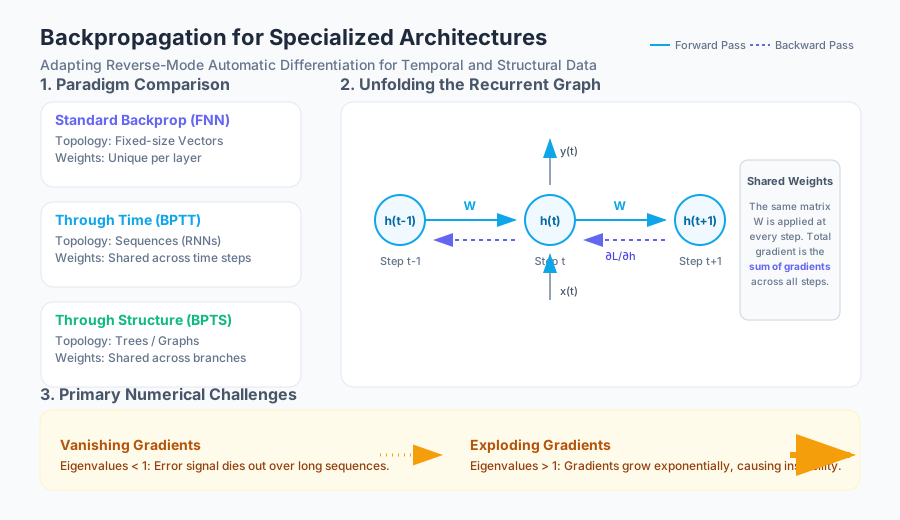
The fundamental algorithm of modern deep learning, Backpropagation, is often misunderstood as a synonym for learning itself. In reality, it is a specific application of Reverse-Mode Automatic Differentiation (AD) designed to compute the gradient of a scalar loss function with respect to the weights of a neural network. While the standard algorithm suffices for Feedforward Neural Networks (FNNs), it encounters significant theoretical and practical hurdles when applied to architectures with temporal dependencies, structural hierarchies, or shared parameters.
To train models like Recurrent Neural Networks (RNNs) or Recursive Neural Networks, we must adapt the backpropagation algorithm to account for parameter sharing and the topology of the data. This article explores the mathematical foundations and implementation nuances of Backpropagation Through Time (BPTT) and Backpropagation Through Structure (BPTS).
AI_SVGI_SVG## The Mathematical Foundation: Chain Rule and Dynamic Programming
At its core, backpropagation is an exercise in the Chain Rule of calculus, optimized via Dynamic Programming. For a composite function $y = f(g(x))$, the derivative is $\frac{dy}{dx} = \frac{dy}{dg} \cdot \frac{dg}{dx}$. In a neural network, this allows us to propagate the "error signal" from the output layer back to the input.
Theorem: The Principle of Reverse-Mode AD Given a computational graph representing a function $f: \mathbb{R}^n \rightarrow \mathbb{R}$, the gradient $\nabla f$ can be computed in a single backward pass with a temporal complexity proportional to the forward pass. This is achieved by caching intermediate partial derivatives (the "forward" values) and multiplying them in reverse order.
Comparison of Backpropagation Paradigms
| Feature | Standard Backprop (FNN) | Backpropagation Through Time (BPTT) | Backpropagation Through Structure (BPTS) |
|---|---|---|---|
| Data Topology | Fixed-size vectors | Sequences (Time-series) | Trees / Graphs |
| Weight Sharing | None (usually) | Across time steps | Across nodes/branches |
| Graph Structure | Static Directed Acyclic Graph (DAG) | Unfolded linear chain | Unfolded tree/recursive structure |
| Primary Challenge | Vanishing Gradients | Long-term dependencies | Structural complexity / Parsing |
Backpropagation Through Time (BPTT)
Backpropagation Through Time (BPTT) is the standard algorithm for training Recurrent Neural Networks (RNNs). Unlike feedforward networks where each layer has its own set of weights, an RNN applies the same weight matrix $W$ at every time step.
1. What it is
BPTT is a technique where the recurrent network is "unfolded" into a deep feedforward network where each layer represents a time step. Because the weights are shared across all time steps, the gradient of the loss with respect to a weight matrix is the sum of the gradients at each time step.
2. Why it matters
RNNs are designed to handle sequential data (speech, text, sensor logs). Without BPTT, we could not compute how a weight update at time $t=0$ affects the loss at time $t=100$. It allows the model to "remember" information by propagating error signals back through the hidden states across the temporal dimension.
3. How it works: The Derivation
Consider a simple RNN with hidden state $h_t$ and input $x_t$: $h_t = \sigma(W_h h_{t-1} + W_x x_t + b)$ $y_t = \text{softmax}(W_y h_t + b_y)$
The total loss $\mathcal{L}$ over $T$ time steps is: $\mathcal{L} = \sum_{t=1}^T \mathcal{L}_t$
To compute the gradient with respect to the recurrent weights $W_h$, we apply the chain rule: $\frac{\partial \mathcal{L}}{\partial W_h} = \sum_{t=1}^T \frac{\partial \mathcal{L}_t}{\partial W_h}$
For a specific time step $t$, the gradient depends on all previous states because $h_t$ is a function of $h_{t-1}$, which is a function of $h_{t-2}$, and so on. $\frac{\partial \mathcal{L}t}{\partial W_h} = \sum{k=1}^t \frac{\partial \mathcal{L}t}{\partial y_t} \frac{\partial y_t}{\partial h_t} \left( \prod{j=k+1}^t \frac{\partial h_j}{\partial h_{j-1}} \right) \frac{\partial h_k}{\partial W_h}$
4. Concrete Example: Truncated BPTT Implementation
In practice, unfolding a network for 1,000 steps leads to memory exhaustion and the Vanishing Gradient Problem. We use Truncated BPTT (TBPTT) to limit the backward pass to a fixed number of steps $k$.
import torch
import torch.nn as nn

class SimpleRNN(nn.Module):
    def __init__(self, input_size, hidden_size):
        super(SimpleRNN, self).__init__()
        self.hidden_size = hidden_size
        self.rnn_cell = nn.RNNCell(input_size, hidden_size)
        self.fc = nn.Linear(hidden_size, 1)

    def forward(self, x, h_prev):
        # x: (batch, seq_len, input_size)
        outputs = []
        h_t = h_prev
        for t in range(x.size(1)):
            h_t = self.rnn_cell(x[:, t, :], h_t)
            outputs.append(self.fc(h_t))
        return torch.stack(outputs, dim=1), h_t

# Training Loop with Truncated BPTT
def train_step(model, data, target, h_prev, k_steps=20):
    # Detach hidden state to prevent backprop beyond k_steps
    h_prev = h_prev.detach()

    output, h_final = model(data, h_prev)
    loss = nn.MSELoss()(output, target)

    loss.backward() # This performs BPTT for the current window
    optimizer.step()
    optimizer.zero_grad()

    return h_final
AI_DEMOI_DEMO### 5. Common Pitfalls: Vanishing and Exploding Gradients The term $\prod_{j=k+1}^t \frac{\partial h_j}{\partial h_{j-1}}$ is the "engine" of BPTT. If the eigenvalues of the weight matrix $W_h$ are less than 1, the gradient shrinks exponentially as it travels back in time (Vanishing Gradient). If they are greater than 1, the gradient grows exponentially (Exploding Gradient).
| Problem | Symptom | Solution |
|---|---|---|
| Exploding Gradients | Loss becomes NaN, weights overflow |
Gradient Clipping (norm scaling) |
| Vanishing Gradients | Model fails to learn long-term dependencies | LSTM/GRU cells, Identity initialization |
| Memory Bottleneck | Out of Memory (OOM) on GPU | Truncated BPTT, Gradient Checkpointing |
Backpropagation Through Structure (BPTS)
While BPTT handles linear sequences, Backpropagation Through Structure (BPTS) generalizes the concept to Recursive Neural Networks (not to be confused with Recurrent). These networks operate on tree-structured data, such as the syntactic parse tree of a sentence or the molecular structure of a chemical compound.
1. What it is
BPTS is an optimization technique for networks where the computational graph is a tree. In a recursive network, a "cell" (similar to an RNN cell) is applied to the children of a node to produce the parent's representation. BPTS propagates the error from the root of the tree down to the leaves.
2. Why it matters
Many real-world phenomena are hierarchical rather than sequential. In Natural Language Processing (NLP), the meaning of a sentence is often better captured by its hierarchical structure (Subject-Verb-Object) than by the linear order of words. BPTS allows the model to learn distributed representations that respect this hierarchy.
3. How it works: The Recursive Step
Let a node $p$ have children $c_1$ and $c_2$. The representation of the parent is: $h_p = \sigma(W [h_{c1}; h_{c2}] + b)$
Where $[h_{c1}; h_{c2}]$ is the concatenation of the children's hidden states. The weight matrix $W$ is shared across all nodes in the tree.
During the backward pass:
- The gradient is received at node $p$ from its parent.
- The gradient is also contributed by the local loss function at node $p$ (if applicable).
- The gradient is backpropagated through the concatenation and the weight matrix $W$ to the children $c_1$ and $c_2$.
- The gradients for $W$ are accumulated across all nodes in the tree.
4. Concrete Example: Sentiment Analysis on a Parse Tree
Imagine a sentence "Not good" parsed as a tree where "Not" and "good" are leaves.
# Pseudocode for BPTS logic
def backprop_through_structure(node, d_loss_d_hp):
    """
    node: current node in the tree
    d_loss_d_hp: gradient of loss w.r.t. current node's hidden state
    """
    if node.is_leaf():
        # Update leaf embeddings
        node.embedding_grad += d_loss_d_hp
        return

    # 1. Compute local gradient w.r.t. weights W
    # h_p = sigma(W * [h_left, h_right] + b)
    combined_children = concat(node.left.h, node.right.h)
    d_W = outer_product(d_loss_d_hp * sigma_prime, combined_children)
    global_W_grad += d_W

    # 2. Propagate gradient to children
    d_children = W.T @ (d_loss_d_hp * sigma_prime)
    d_left, d_right = split(d_children)

    # 3. Recursive calls
    backprop_through_structure(node.left, d_left)
    backprop_through_structure(node.right, d_right)
5. Variations: Tree-LSTMs
Standard BPTS suffers from the same vanishing gradient issues as RNNs. To solve this, researchers developed the Tree-LSTM, which applies the LSTM gating mechanism to tree structures. In a Tree-LSTM, a parent node has a "forget gate" for each child, allowing it to selectively retain or discard information from specific branches of the hierarchy.
Advanced Gradient Management
Training specialized architectures requires more than just the basic algorithm. Several techniques are essential to ensure convergence.
Gradient Clipping
To prevent exploding gradients in BPTT, we scale the gradient if its norm exceeds a threshold $\tau$: $\text{if } |\nabla \mathcal{L}| > \tau: \nabla \mathcal{L} \leftarrow \tau \frac{\nabla \mathcal{L}}{|\nabla \mathcal{L}|}$
Gradient Checkpointing
For extremely long sequences or massive trees, storing all intermediate activations for the backward pass is impossible. Gradient Checkpointing trades computation for memory by only storing activations for a subset of nodes (checkpoints) and re-computing the intermediate activations during the backward pass.
Complexity Analysis
| Algorithm | Time Complexity (Forward) | Time Complexity (Backward) | Space Complexity |
|---|---|---|---|
| Standard Backprop | $O(N)$ | $O(N)$ | $O(N)$ |
| BPTT | $O(T \times H^2)$ | $O(T \times H^2)$ | $O(T \times H)$ |
| Truncated BPTT | $O(T \times H^2)$ | $O(k \times H^2)$ | $O(k \times H)$ |
| BPTS | $O(N \times H^2)$ | $O(N \times H^2)$ | $O(\text{depth} \times H)$ |
(Where $N$ is nodes/layers, $T$ is time steps, $H$ is hidden size, and $k$ is truncation window.)
Backpropagation in Graph Neural Networks (GNNs)
Modern specialized architectures often involve graphs that are neither linear nor tree-like. GNNs use a form of backpropagation that operates on Message Passing phases.
In a GNN, the "forward pass" involves nodes aggregating features from their neighbors. The "backward pass" must propagate gradients through these aggregations. If the graph is static, this is equivalent to backpropagation through a very large, sparse computational graph. If the graph is dynamic or contains cycles, techniques similar to BPTT (iterative message passing) are used, often requiring the system to reach a fixed point or using a fixed number of iterations.
Key Insight: Backpropagation through any specialized architecture is essentially the process of defining a topological sort of the computational graph and applying the chain rule in reverse order. The "specialization" lies in how we handle shared parameters and how we manage the memory of intermediate states.
Summary of Best Practices
- Initialize Carefully: For BPTT, initializing the recurrent weight matrix $W_h$ as an identity matrix or using orthogonal initialization can significantly mitigate vanishing gradients.
- Monitor Norms: Always track the $L_2$ norm of your gradients. Sudden spikes are a precursor to divergence.
- Use Frameworks: While understanding the derivation is crucial, use autograd engines (PyTorch, JAX, TensorFlow). They handle the complex bookkeeping of shared weights and structural unfolding more efficiently than manual implementations.
- Batching: Batching tree structures (BPTS) is significantly harder than batching sequences (BPTT). Use libraries like
DGL(Deep Graph Library) orPyTorch Geometricwhich implement specialized batching kernels for non-linear structures.
AI_STUDY_GUIDEI_STUDY_GUIDE### Flashcards (Conceptual)
- Q: What is the main difference between Backpropagation and BPTT?
- A: Standard backpropagation assumes independent weights per layer, while BPTT handles shared weights across time steps by summing gradients across the temporal unfolding.
- Q: Why is Truncated BPTT used?
- A: To reduce memory consumption and prevent the vanishing gradient problem from becoming unmanageable over very long sequences.
- Q: In BPTS, how are weight updates calculated?
- A: The gradient is calculated at each node in the tree structure, and because the weights are shared across all nodes, the individual gradients are summed to produce the final update.
- Q: What is the "Jacobian" in the context of BPTT?
- A: It is the matrix of partial derivatives of the hidden state at time $t$ with respect to the hidden state at time $t-1$. Its eigenvalues determine gradient stability.
Quiz: Backpropagation Mastery
- True/False: In BPTT, the number of layers in the unfolded network is equal to the number of time steps in the input sequence.
- Multiple Choice: Which technique is specifically designed to handle the "Exploding Gradient" problem?
- A) Dropout
- B) Gradient Clipping
- C) Batch Normalization
- D) Xavier Initialization
- Short Answer: Explain why recursive neural networks (BPTS) are more computationally expensive to batch than recurrent neural networks (BPTT).
- Calculation: If an RNN has a sequence length of 3, and the gradient of the loss w.r.t the hidden state at each step is $\delta_1, \delta_2, \delta_3$, write the simplified expression for the total gradient w.r.t the shared weight $W$.
Study Guide: Specialized Backpropagation
- Core Concept: Backpropagation is Reverse-Mode AD.
- BPTT Focus: Temporal unfolding, weight sharing across time, vanishing/exploding gradients, TBPTT.
- BPTS Focus: Structural unfolding (trees), recursive application of weights, hierarchical representations.
- Implementation: Use
detach()for truncation, usesum()for shared weight gradients, useclip_grad_norm_for stability. - Further Reading: Rumelhart et al. (1986) for the original backprop; Hochreiter (1991) for vanishing gradients; Goller & Küchler (1996) for BPTS.
Source Materials
Study Backpropagation on Lykke
This course page is free to open: signed out, you can read its first two sections, and signing in, on any plan, opens the rest. The free Lykke Chrome extension syncs your own Canvas courses, so ChatGPT, Claude and Muse can answer from your classes and deadlines. It only reads Canvas.
Add the free extensionSign in to open every section