From the free course Backpropagation on Lykke
Advanced Optimization and Efficiency
Key concepts: Levenberg–Marquardt (LM) algorithm · Quasi-Hessian matrix · Jacobian matrix storage · Second-order training
Methods to improve the speed and memory efficiency of backpropagation-based training.
Advanced Optimization and Efficiency
In the landscape of machine learning, the transition from theoretical models to production-ready systems is governed by the efficiency of optimization. While the fundamental goal remains the minimization of a loss function $L(\theta)$, the path to that minimum is fraught with computational bottlenecks, vanishing signals, and memory constraints. Advanced optimization focuses on two fronts: the algorithmic efficiency of gradient computation across diverse architectures and the convergence speed provided by higher-order mathematical approximations.
AI_SVGI_SVG## The Foundation: Backpropagation as Reverse-Mode AD
At its core, Backpropagation is an application of the chain rule from calculus, optimized through Dynamic Programming. While often conflated with the entire training process, it is strictly a method for calculating the gradient of a loss function with respect to the weights of a neural network.
1. What it is
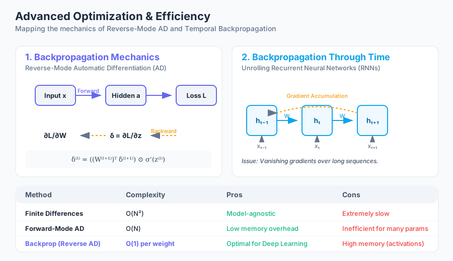
Backpropagation is a specific case of Reverse-Mode Automatic Differentiation (AD). It computes the partial derivatives $\frac{\partial L}{\partial w_{ij}}$ by traversing the computational graph from the output back to the input.
Definition: Backpropagation is an efficient algorithm for computing the gradient of a scalar-valued function of multiple variables, specifically designed for functions represented as a directed acyclic graph (DAG) of elementary operations.
2. Why it matters
Before backpropagation became widely recognized in the mid-1980s (notably by Rumelhart, Hinton, and Williams), training deep networks was considered computationally intractable. A naive approach would require $O(N)$ forward passes to compute gradients for $N$ parameters via finite differences. Backpropagation reduces this to a single backward pass, making the complexity $O(1)$ relative to the forward pass cost per parameter.
3. How it works: The Mechanics
The algorithm operates in two distinct phases:
- Forward Pass: Input data is propagated through the network. At each node, the intermediate activations $a^{(l)}$ and pre-activations $z^{(l)}$ are stored.
- Backward Pass: The "error" signal $\delta^{(l)}$ is computed starting from the output layer.
Mathematically, for a layer $l$: $$z^{(l)} = W^{(l)}a^{(l-1)} + b^{(l)}$$ $$a^{(l)} = \sigma(z^{(l)})$$
The gradient for the weights is: $$\frac{\partial L}{\partial W^{(l)}} = \delta^{(l)} (a^{(l-1)})^T$$ Where the error $\delta$ is propagated backward: $$\delta^{(l)} = ((W^{(l+1)})^T \delta^{(l+1)}) \odot \sigma'(z^{(l)})$$
4. Comparison of Computational Approaches
| Method | Complexity | Pros | Cons |
|---|---|---|---|
| Finite Differences | $O(N^2)$ | Simple to implement, model-agnostic | Extremely slow for large $N$ |
| Forward-Mode AD | $O(N)$ | Low memory overhead | Inefficient for many parameters, one output |
| Backpropagation (Reverse-Mode) | $O(1)$ per weight | Highly efficient for many parameters | High memory (must store all activations) |
5. Implementation Example (Python/NumPy)
import numpy as np

def sigmoid(x):
    return 1 / (1 + np.exp(-x))

def sigmoid_derivative(x):
    return x * (1 - x)

def backprop_step(x, y, weights_input_hidden, weights_hidden_output):
    # 1. Forward Pass
    hidden_layer_input = np.dot(x, weights_input_hidden)
    hidden_layer_output = sigmoid(hidden_layer_input)

    output_layer_input = np.dot(hidden_layer_output, weights_hidden_output)
    predicted_output = sigmoid(output_layer_input)

    # 2. Compute Output Error
    error = y - predicted_output
    d_predicted_output = error * sigmoid_derivative(predicted_output)

    # 3. Backpropagate to Hidden Layer
    error_hidden_layer = d_predicted_output.dot(weights_hidden_output.T)
    d_hidden_layer = error_hidden_layer * sigmoid_derivative(hidden_layer_output)

    # 4. Gradient Calculation
    grad_weights_hidden_output = hidden_layer_output.T.dot(d_predicted_output)
    grad_weights_input_hidden = x.T.dot(d_hidden_layer)

    return grad_weights_input_hidden, grad_weights_hidden_output
Temporal Dynamics: Backpropagation Through Time (BPTT)
When dealing with sequential data, standard backpropagation fails because the network's state at time $t$ depends on its state at $t-1$. Backpropagation Through Time (BPTT) solves this by "unfolding" the recurrent neural network (RNN).
1. What it is
BPTT is the application of the backpropagation algorithm to a Recurrent Neural Network that has been unrolled into a deep feedforward network where each layer represents a time step and all layers share the same parameters.
2. Why it matters
RNNs are essential for time-series, speech, and natural language. However, the shared weight matrix $W$ is applied repeatedly. This creates a deep dependency chain, leading to the Vanishing/Exploding Gradient Problem, where the gradient signal either disappears or grows exponentially as it travels back through many time steps.
3. Mechanics of Unfolding
Consider a hidden state $h_t = \sigma(W_h h_{t-1} + W_x x_t)$. To compute the gradient of the loss $L$ at time $T$ with respect to $W_h$: $$\frac{\partial L_T}{\partial W_h} = \sum_{t=1}^T \frac{\partial L_T}{\partial h_T} \frac{\partial h_T}{\partial h_t} \frac{\partial h_t}{\partial W_h}$$
The term $\frac{\partial h_T}{\partial h_t}$ involves a product of Jacobian matrices: $$\frac{\partial h_T}{\partial h_t} = \prod_{k=t+1}^T \frac{\partial h_k}{\partial h_{k-1}}$$
4. Variations of BPTT
| Variation | Description | Use Case |
|---|---|---|
| Full BPTT | Unfolds the network for the entire sequence length. | Short sequences, high precision. |
| Truncated BPTT | Unfolds for a fixed number of steps $k$, then stops. | Long sequences (e.g., character-level language models). |
| Real-Time Recurrent Learning (RTRL) | Computes gradients forward in time. | Online learning where sequences are infinite. |
5. Common Pitfalls: The Vanishing Gradient
In BPTT, if the eigenvalues of the weight matrix $W_h$ are less than 1, the product $\prod \frac{\partial h_k}{\partial h_{k-1}}$ will shrink to zero.
- Symptom: The model fails to learn long-term dependencies (e.g., the beginning of a sentence doesn't affect the end).
- Solution: Use Gated architectures (LSTM, GRU) or Gradient Clipping.
AI_DEMOI_DEMO--
Structural Generalization: Backpropagation Through Structure (BPTS)
While BPTT handles linear sequences, Backpropagation Through Structure (BPTS) extends the concept to recursive structures, such as trees or graphs.
1. What it is
BPTS is a gradient-based technique for training Recursive Neural Networks. Unlike Recurrent networks (linear), Recursive networks process data in a hierarchical fashion (e.g., a parse tree of a sentence).
2. Why it matters
In Natural Language Processing, sentences have a nested, hierarchical structure. BPTS allows the model to learn distributed representations of phrases and sentences by following the syntax tree, rather than just the word order.
3. How it works
- Topology: The network structure is defined by the input (e.g., a binary tree).
- Forward Pass: Nodes are computed from leaves to root.
- Backward Pass: Gradients are propagated from the root down to the leaves. If a weight $W$ is used at multiple nodes in the tree, the total gradient is the sum of gradients at each node.
4. Comparison: BPTT vs. BPTS
| Feature | BPTT (Recurrent) | BPTS (Recursive) |
|---|---|---|
| Data Structure | Linear Sequence | Tree / DAG |
| Dependency | Temporal (Time $t$) | Structural (Parent/Child) |
| Complexity | $O(T)$ where $T$ is length | $O(N)$ where $N$ is number of nodes |
| Primary Application | Speech, Sensors | NLP Parsing, Chemistry (Molecules) |
Second-Order Optimization: The Levenberg–Marquardt (LM) Algorithm
Standard backpropagation uses first-order derivatives (the gradient). However, first-order methods can be slow to converge near local minima. Second-order methods use the Hessian matrix (second derivatives) to find the optimal step size and direction.
1. What it is
The Levenberg–Marquardt (LM) algorithm is an optimization technique that interpolates between the Gauss-Newton algorithm and the method of Gradient Descent. It is specifically designed for least-squares problems.
2. Why it matters
LM is significantly faster than standard gradient descent for small-to-medium-sized neural networks. It avoids the "zig-zagging" behavior of first-order methods in narrow valleys of the loss surface.
3. Mechanics and the Quasi-Hessian
The update rule for LM is: $$\theta_{k+1} = \theta_k - [J^T J + \mu I]^{-1} J^T e$$
Where:
- $J$ is the Jacobian matrix containing first derivatives of the errors with respect to parameters.
- $J^T J$ is the Quasi-Hessian approximation.
- $e$ is the vector of network errors.
- $\mu$ is the damping factor.
Key Insight: When $\mu$ is large, the algorithm behaves like Gradient Descent with a small step size. When $\mu$ is small (or zero), it behaves like the Gauss-Newton method, which has quadratic convergence properties.
4. Comparison of Optimization Methods
| Method | Update Rule | Convergence Speed | Memory Cost |
|---|---|---|---|
| Gradient Descent | $-\alpha \nabla L$ | Linear | Low ($O(N)$) |
| Newton's Method | $-H^{-1} \nabla L$ | Quadratic | Very High ($O(N^2)$) |
| Levenberg-Marquardt | $-(J^T J + \mu I)^{-1} J^T e$ | Super-linear | High ($O(N^2)$) |
5. Memory Efficiency in LM
The primary bottleneck of LM is storing the Jacobian $J$ and inverting the matrix $J^T J$. For a network with $N$ parameters and $M$ training patterns, $J$ is an $M \times N$ matrix. Modern implementations use Jacobian-free products or Memory-Efficient LM which calculates $J^T J$ and $J^T e$ incrementally: $$J^T J = \sum_{i=1}^M j_i j_i^T$$ This allows the algorithm to run without ever storing the full Jacobian matrix in memory.
Synthesis: Choosing the Right Optimizer
Efficiency in deep learning is not a "one size fits all" solution. The choice of algorithm depends on the architecture and the scale of the data.
- For Massive Scale (LLMs, Vision Transformers): First-order methods with momentum (Adam, AdamW) are preferred. The $O(N^2)$ memory cost of second-order methods like LM is prohibitive when $N$ is in the billions.
- For High Precision (Control Systems, Shallow Networks): LM is superior. It converges in far fewer iterations and can find much more precise minima.
- For Structured Data (Code, Syntax): BPTS is necessary to capture the recursive nature of the input, even if it is more complex to implement than BPTT.
Summary of Efficiency Trade-offs
| Scenario | Recommended Approach | Reason |
|---|---|---|
| Real-time streaming data | Truncated BPTT | Limits memory usage and latency. |
| Small dataset, high accuracy needed | Levenberg-Marquardt | Faster convergence to global/local minima. |
| Standard Deep Learning | Backprop + Adam | Best balance of speed and memory. |
| Hierarchical/Nested data | BPTS | Captures structural dependencies. |
AI_STUDY_GUIDEI_STUDY_GUIDE## Study Guide: Advanced Optimization and Efficiency
Core Concepts to Master
- Reverse-Mode AD: Understand why backpropagation is a dynamic programming problem. Be able to derive the gradient for a single neuron.
- The Unfolding Process: Visualize how an RNN becomes a deep feedforward network. Understand that $W$ is the same at every layer.
- Vanishing Gradients: Explain why the product of many small numbers leads to zero and how this kills learning in BPTT.
- The Jacobian vs. The Hessian: Know that the Jacobian is first-order (slopes) and the Hessian is second-order (curvature).
- Damping Factor ($\mu$): Explain how $\mu$ in the LM algorithm switches the strategy between Gradient Descent and Gauss-Newton.
Mathematical Identities to Remember
- Chain Rule: $\frac{dz}{dx} = \frac{dz}{dy} \cdot \frac{dy}{dx}$
- LM Update: $\Delta \theta = (J^T J + \mu I)^{-1} J^T e$
- RNN State: $h_t = f(Wh_{t-1} + Ux_t)$
Practical Application Tips
- When using BPTT, always monitor the norm of the gradients. If they exceed a threshold, use Gradient Clipping.
- If your model is not converging with SGD, try a second-order approximation like L-BFGS or LM if the parameter count allows.
- For BPTS, ensure your input data is pre-processed into a consistent tree structure (e.g., using a Penn Treebank parser).
Source Materials
Study Backpropagation on Lykke
This course page is free to open: signed out, you can read its first two sections, and signing in, on any plan, opens the rest. The free Lykke Chrome extension syncs your own Canvas courses, so ChatGPT, Claude and Muse can answer from your classes and deadlines. It only reads Canvas.
Add the free extensionSign in to open every section