From the free course Applied Linear Algebra and Least Squares on Lykke
Linear Functions, Norms, and Distance
Key concepts: Superposition · Euclidean norm · Triangle inequality · Cauchy-Schwarz inequality · RMS value
Explores linear functions via superposition and measures of magnitude and distance using the Euclidean norm.
Linear Functions, Norms, and Distance
In the study of applied linear algebra, the transition from basic vector arithmetic to functional analysis marks a critical shift in perspective. While vectors can be viewed simply as lists of numbers, their true power is unlocked when we treat them as inputs to linear functions and measure their geometric properties through norms and distances. This section establishes the rigorous mathematical foundation for understanding how vectors interact within a space, how we quantify their magnitude, and how we define the "closeness" of data points—concepts that underpin everything from signal processing to modern machine learning.
Linear Functions
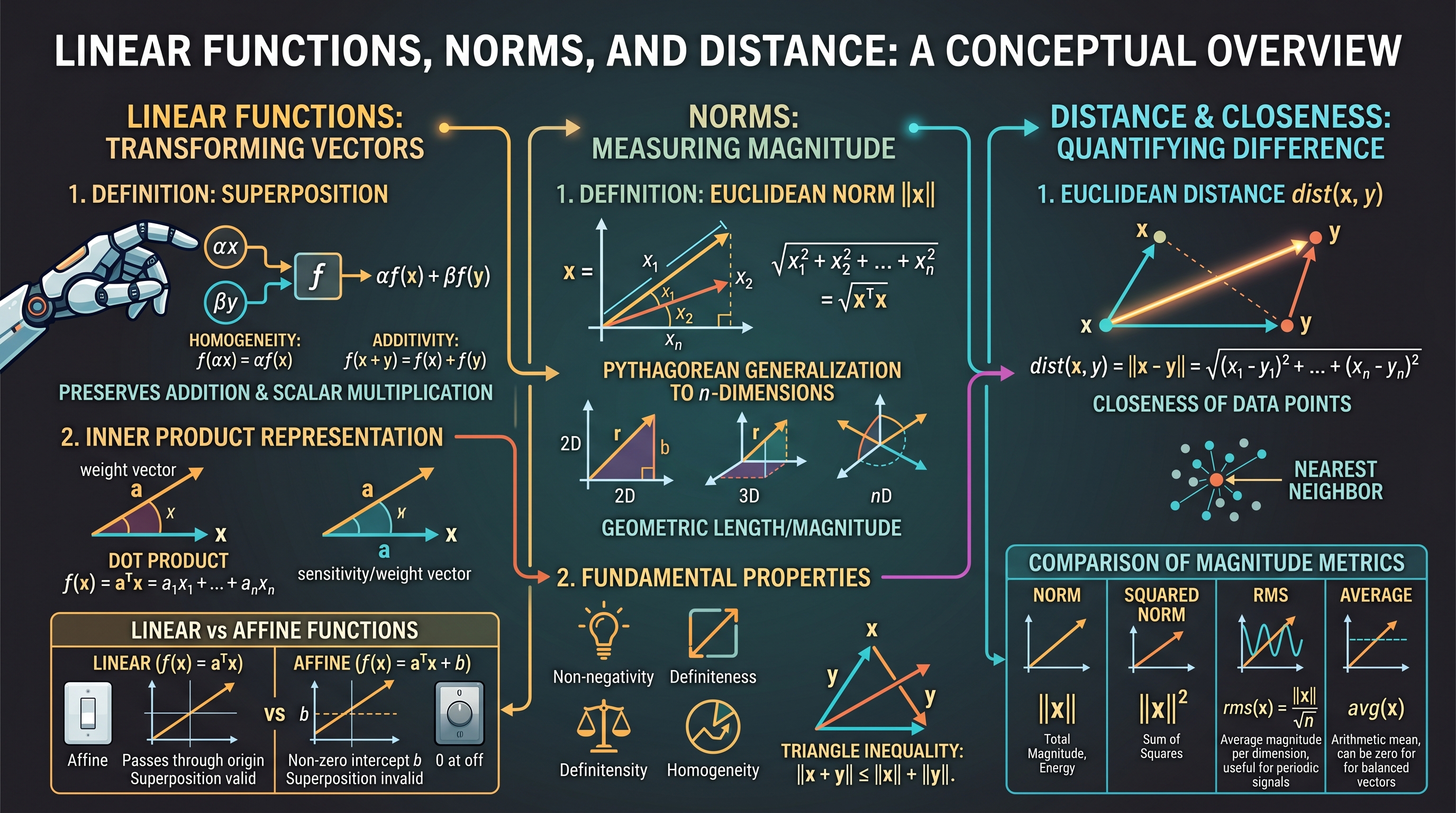
A function $f: \mathbb{R}^n \to \mathbb{R}$ is considered linear if it preserves the operations of addition and scalar multiplication. This is captured by the superposition property, which is the defining characteristic of linearity in any system.
The Superposition Property
The principle of superposition states that the response of a linear system to a weighted sum of inputs is the same as the weighted sum of the responses to those individual inputs. Mathematically, a function $f$ is linear if for all vectors $x, y$ and all scalars $\alpha, \beta$:
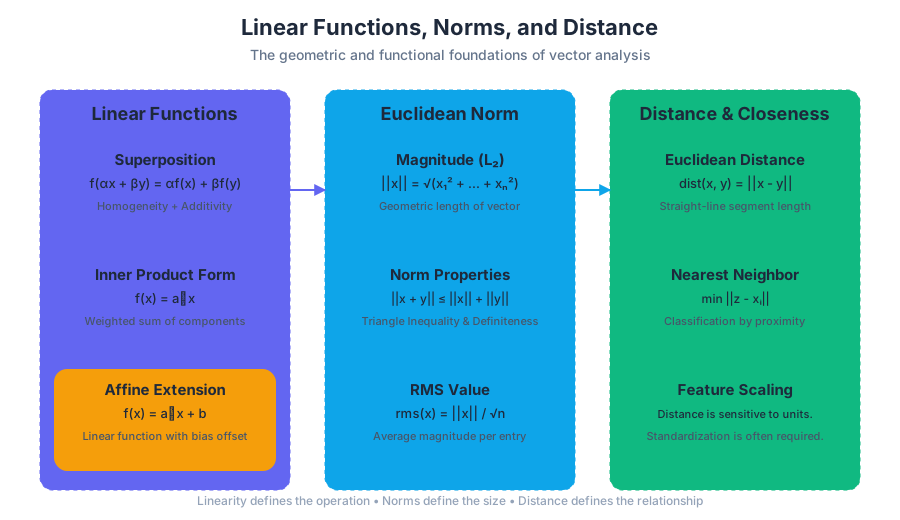
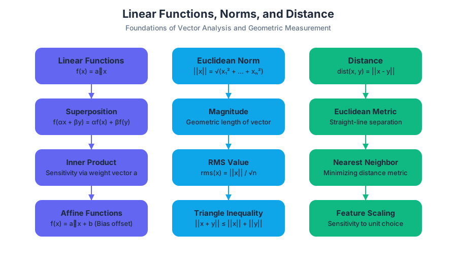
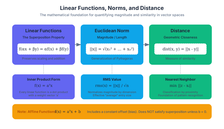
Definition: Superposition $$f(\alpha x + \beta y) = \alpha f(x) + \beta f(y)$$
This property can be decomposed into two distinct requirements:
- Homogeneity: $f(\alpha x) = \alpha f(x)$ (scaling the input scales the output).
- Additivity: $f(x + y) = f(x) + f(y)$ (the output of a sum is the sum of the outputs).
Inner Product Representation
One of the most profound results in finite-dimensional linear algebra is that every linear function $f: \mathbb{R}^n \to \mathbb{R}$ can be expressed as an inner product with some fixed vector $a$. This means that for any linear function, there exists a unique vector $a$ such that: $$f(x) = a^Tx = a_1x_1 + a_2x_2 + \dots + a_nx_n$$ In this context, the vector $a$ is often called the weight vector or the coefficient vector. Each component $a_i$ represents the sensitivity of the function's output to changes in the corresponding input $x_i$.
Affine Functions
In practice, many functions we encounter are not strictly linear but are affine. An affine function is a linear function plus a constant offset: $$f(x) = a^Tx + b$$ where $b$ is a scalar called the bias or offset. While affine functions do not satisfy the superposition property (unless $b=0$), they are often colloquially referred to as "linear" in fields like regression and neural networks.
| Feature | Linear Function ($f(x) = a^Tx$) | Affine Function ($f(x) = a^Tx + b$) |
|---|---|---|
| Passes through origin? | Yes ($f(0) = 0$) | No (unless $b=0$) |
| Superposition? | Valid | Invalid |
| Homogeneity? | Valid | Invalid |
| Additivity? | Valid | Invalid |
| Constant Term? | Always 0 | Any real number $b$ |
The Euclidean Norm
While the inner product gives us a way to relate two vectors, the norm gives us a way to measure a single vector. The Euclidean norm (also known as the $L_2$ norm) is the standard geometric measure of a vector's "length" or "magnitude."
Definition and Calculation
The Euclidean norm of an $n$-vector $x$ is denoted by $|x|$ and is defined as the square root of the sum of the squares of its components:
Definition: Euclidean Norm $$|x| = \sqrt{x_1^2 + x_2^2 + \dots + x_n^2} = \sqrt{x^Tx}$$
This definition is a direct generalization of the Pythagorean theorem from 2D and 3D space to $n$-dimensional space.
Fundamental Properties of Norms
For any vector $x$ and scalar $\alpha$, the Euclidean norm satisfies several critical properties:
- Non-negativity: $|x| \ge 0$.
- Definiteness: $|x| = 0$ if and only if $x = 0$.
- Homogeneity: $|\alpha x| = |\alpha| |x|$.
- Triangle Inequality: $|x + y| \le |x| + |y|$.
Root Mean Square (RMS) Value
In many engineering applications, particularly those involving periodic signals or large datasets, the norm can become very large as the dimension $n$ increases. To normalize for the number of components, we use the RMS value: $$rms(x) = \frac{|x|}{\sqrt{n}} = \sqrt{\frac{x_1^2 + \dots + x_n^2}{n}}$$ The RMS value provides a measure of the "typical" size of an entry in the vector. For example, if a vector represents a voltage signal over time, the RMS value represents the effective constant voltage that would deliver the same power.
| Metric | Formula | Interpretation |
|---|---|---|
| Norm $|x|$ | $\sqrt{\sum x_i^2}$ | Total magnitude / "Length" |
| Squared Norm $|x|^2$ | $\sum x_i^2$ | Energy / Sum of Squares |
| RMS $rms(x)$ | $|x| / \sqrt{n}$ | Average magnitude per dimension |
| Average $avg(x)$ | $(\sum x_i) / n$ | Arithmetic mean (can be zero for large $x$) |
Distance and Closeness
The concept of "distance" allows us to quantify how similar or different two vectors are. In the Euclidean framework, the distance between two vectors $x$ and $y$ is simply the norm of their difference.
Euclidean Distance
The distance $dist(x, y)$ is defined as: $$dist(x, y) = |x - y| = \sqrt{(x_1 - y_1)^2 + \dots + (x_n - y_n)^2}$$ This represents the length of the straight-line segment connecting the points $x$ and $y$ in $n$-dimensional space.
Applications: Nearest Neighbor Classification
Distance is the fundamental metric used in Nearest Neighbor (NN) algorithms. Given a set of "training" vectors $x_1, \dots, x_N$ with known labels, and a new "test" vector $z$, the NN algorithm finds the training vector $x_i$ that minimizes $|z - x_i|$.
- Feature Vectors: In this context, vectors represent "features" of an object (e.g., height, weight, age).
- Scaling: It is crucial to note that distance is sensitive to the units of the components. If one component is measured in millimeters and another in kilometers, the kilometer-scale component will dominate the distance calculation. This necessitates feature scaling or standardization.
The Cauchy-Schwarz Inequality
The Cauchy-Schwarz inequality is one of the most important inequalities in all of mathematics. It relates the inner product of two vectors to the product of their norms.
Theorem: Cauchy-Schwarz Inequality For any $n$-vectors $a$ and $b$: $$|a^Tb| \le |a| |b|$$
Implications and Equality Conditions
The inequality tells us that the absolute value of the inner product can never exceed the product of the lengths of the vectors.
- Equality: The equality $|a^Tb| = |a| |b|$ holds if and only if $a$ and $b$ are linearly dependent (i.e., one is a scalar multiple of the other, $a = \beta b$ or $b = \beta a$).
- Upper Bound: It provides a way to bound the output of a linear function. If $f(x) = a^Tx$, then $|f(x)| \le |a| |x|$.
The Triangle Inequality
A direct consequence of the Cauchy-Schwarz inequality is the Triangle Inequality: $$|x + y| \le |x| + |y|$$ Geometrically, this states that the length of one side of a triangle cannot exceed the sum of the lengths of the other two sides. In the context of vectors, it means that the "shortcut" (the vector sum $x+y$) is always shorter than or equal to the path taken by traveling along $x$ and then along $y$.
| Inequality | Mathematical Statement | Geometric/Physical Meaning |
|---|---|---|
| Cauchy-Schwarz | $ | x^Ty |
| Triangle Inequality | $|x+y| \le |x| + |y|$ | The straight line is the shortest path. |
| Reverse Triangle | $|x-y| \ge | |x| - |y| |
Angles and Orthogonality
By combining the inner product and the norm, we can define the angle between two vectors in $\mathbb{R}^n$, extending our 3D intuition to arbitrary dimensions.
Defining the Angle
The angle $\theta$ between two non-zero vectors $a$ and $b$ is defined as: $$\cos \theta = \frac{a^Tb}{|a| |b|}$$ Because of the Cauchy-Schwarz inequality, the term on the right is always between $-1$ and $1$, ensuring that a unique angle $\theta \in [0, \pi]$ always exists.
Orthogonality
Two vectors are said to be orthogonal if their inner product is zero: $$a^Tb = 0 \iff a \perp b$$ In geometric terms, orthogonal vectors are at a $90^\circ$ angle to each other. This is a central concept in linear algebra, leading to the development of orthonormal bases and projections.
Correlation Coefficient
In statistics, the correlation coefficient $\rho$ between two vectors of data (with zero mean) is exactly the cosine of the angle between them.
- If $\theta = 0$ ($\cos \theta = 1$), the vectors are perfectly correlated.
- If $\theta = \pi$ ($\cos \theta = -1$), the vectors are perfectly negatively correlated.
- If $\theta = \pi/2$ ($\cos \theta = 0$), the vectors are uncorrelated (orthogonal).
Common Pitfalls and Misconceptions
Even experienced practitioners can stumble on the nuances of norms and linear functions.
- Linear vs. Affine Confusion: In many software libraries (like scikit-learn), a "Linear Regression" model actually fits an affine function ($y = ax + b$). Forgetting the bias term $b$ in a purely linear model can lead to poor fits if the data does not pass through the origin.
- The "Square Root" Oversight: When calculating the Euclidean norm, beginners often forget to take the square root of the sum of squares, resulting in the squared norm $|x|^2$. While the squared norm is useful (and computationally cheaper), it does not satisfy the triangle inequality or the homogeneity property of a true norm.
- Dimensionality and Distance: In very high dimensions, the concept of "distance" becomes counter-intuitive. In a phenomenon known as the curse of dimensionality, the distance between any two random points in a high-dimensional cube tends to become almost equal, making "nearest neighbor" searches less effective.
- RMS vs. Average: The RMS value is always greater than or equal to the absolute value of the average. $rms(x) \ge |avg(x)|$. Using the average to describe the "magnitude" of a signal like a sine wave is useless (as the average is zero), whereas the RMS provides the correct physical context of power.
Summary of Key Formulas
| Concept | Formula |
|---|---|
| Linear Function | $f(x) = a^Tx$ |
| Euclidean Norm | $|x| = \sqrt{\sum x_i^2}$ |
| RMS Value | $rms(x) = |x| / \sqrt{n}$ |
| Distance | $dist(x, y) = |x - y|$ |
| Cauchy-Schwarz | $ |
| Angle ($\theta$) | $\cos \theta = (x^Ty) / (|x| |y|)$ |
Source Materials
Study Applied Linear Algebra and Least Squares on Lykke
This course page is free to open: signed out, you can read its first two sections, and signing in, on any plan, opens the rest. The free Lykke Chrome extension syncs your own Canvas courses, so ChatGPT, Claude and Muse can answer from your classes and deadlines. It only reads Canvas.
Add the free extensionSign in to open every sectionAll sections of Applied Linear Algebra and Least Squares · Browse more course pages