From the free course Applied Linear Algebra and Least Squares on Lykke
Nonlinear Least Squares
Key concepts: Gauss-Newton algorithm · Levenberg-Marquardt algorithm · Augmented Lagrangian · Penalty algorithm
Introduces iterative algorithms for solving least squares problems where the model is nonlinear.
Nonlinear Least Squares
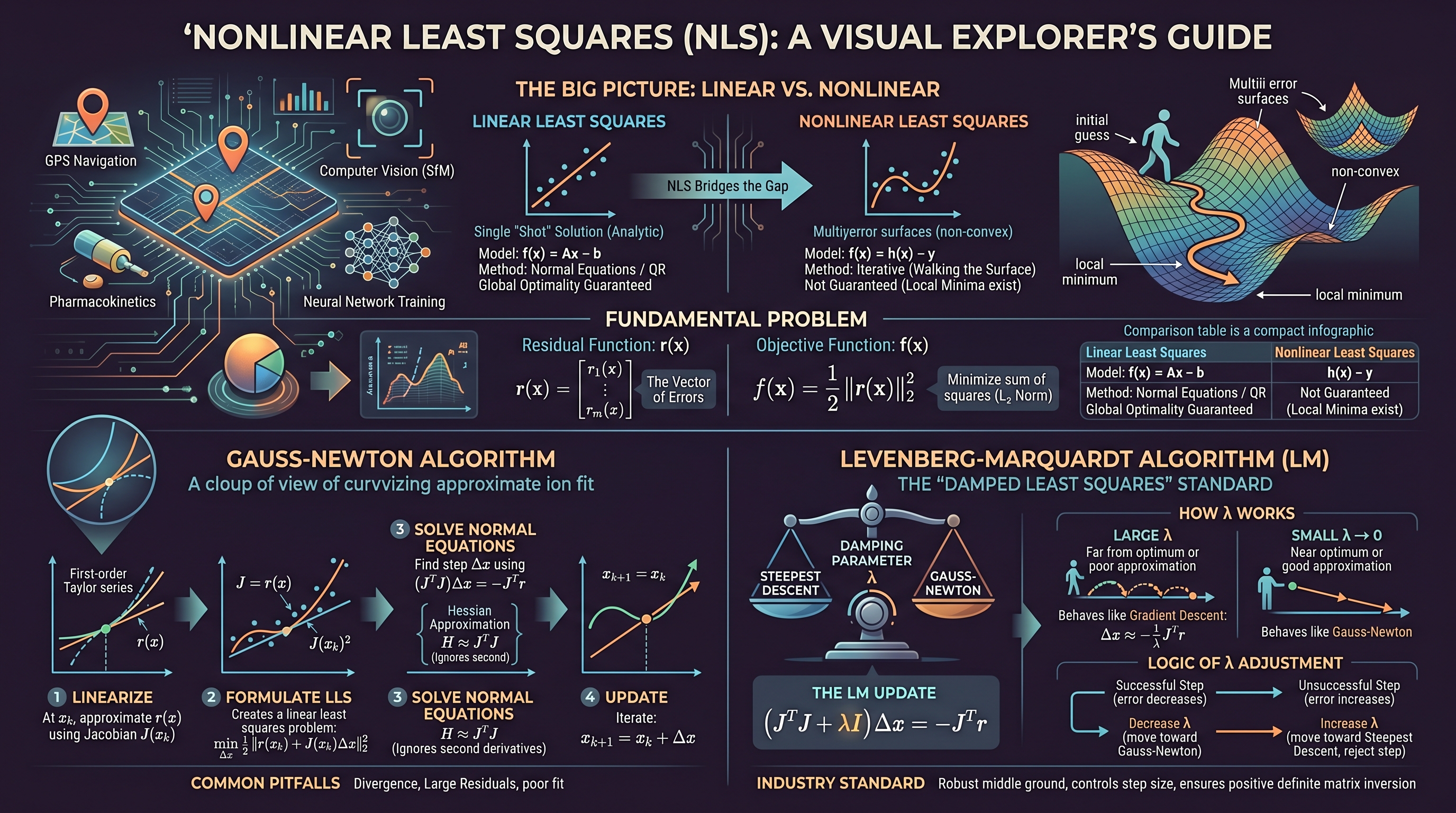
In the landscape of mathematical optimization, Nonlinear Least Squares (NLS) represents the bridge between the simple, closed-form solutions of linear regression and the complex, iterative world of general non-convex optimization. While linear least squares can be solved in a single "shot" using the Normal Equations or QR factorization, NLS arises when the model function depends nonlinearly on the parameters. This is the standard regime for real-world problems ranging from satellite navigation (GPS) and computer vision (Structure from Motion) to pharmacokinetics and neural network training.
The Fundamental Problem
The goal of Nonlinear Least Squares is to find a parameter vector $x \in \mathbb{R}^n$ that minimizes the sum of the squares of the errors (residuals) between observed data and a nonlinear model.
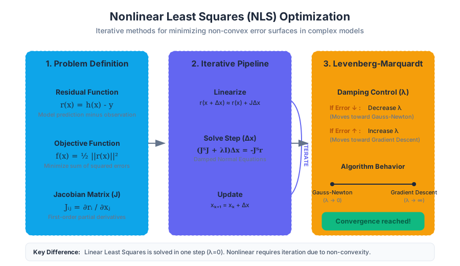
Formally, we define the residual function $r: \mathbb{R}^n \to \mathbb{R}^m$ (where $m \geq n$): $$r(x) = \begin{bmatrix} r_1(x) \ r_2(x) \ \vdots \ r_m(x) \end{bmatrix}$$ The objective function to minimize is the squared $L_2$ norm of these residuals: $$f(x) = \frac{1}{2} |r(x)|^2_2 = \frac{1}{2} \sum_{i=1}^m r_i(x)^2$$
Unlike linear least squares, where $r(x) = Ax - b$, the nonlinear nature of $r(x)$ means $f(x)$ is generally non-convex. This implies the existence of multiple local minima, and our algorithms must iteratively "walk" down the error surface from an initial guess $x_0$.
| Feature | Linear Least Squares | Nonlinear Least Squares |
|---|---|---|
| Model Form | $f(x) = Ax - b$ | $f(x) = h(x) - y$ |
| Solution Method | Analytic (Normal Equations, QR) | Iterative (Gauss-Newton, LM) |
| Complexity | $O(mn^2)$ | $O(K \cdot mn^2)$ where $K$ is iterations |
| Global Optimality | Guaranteed (if $A$ is full rank) | Not guaranteed (depends on $x_0$) |
| Requirements | Linear independence | Differentiability of $r(x)$ |
Gauss-Newton Algorithm
The Gauss-Newton Algorithm is the foundational iterative method for solving NLS. It is a modification of Newton's method for optimization that avoids the computational burden of calculating the second derivatives (the Hessian matrix) of the residual functions.
1. What it is
Gauss-Newton is an iterative descent method that linearizes the residual function $r(x)$ around the current estimate $x_k$ using a first-order Taylor expansion and then solves the resulting linear least squares problem.
2. Why it matters
In pure Newton's method, the Hessian $H$ of $f(x)$ is required: $$H(x) = J(x)^T J(x) + \sum_{i=1}^m r_i(x) \nabla^2 r_i(x)$$ Calculating $\nabla^2 r_i(x)$ is often computationally expensive or analytically impossible. Gauss-Newton assumes the second-term (the sum of residuals times their second derivatives) is small enough to be ignored, particularly when the residuals $r_i(x)$ are near zero (a "good fit").
3. How it works
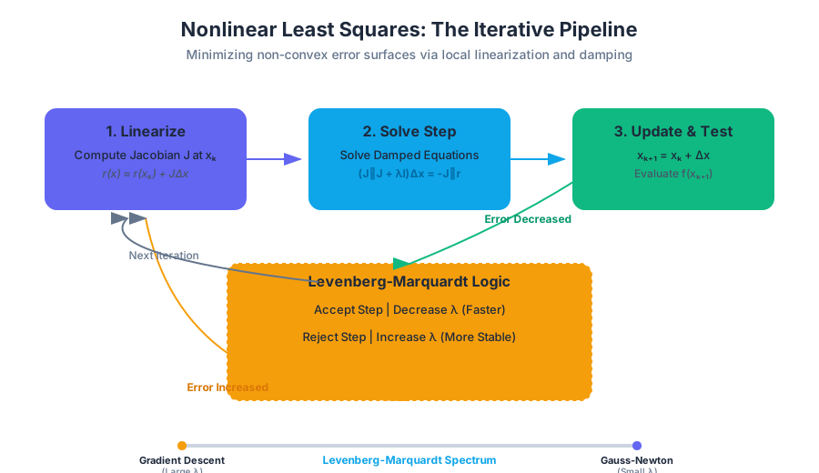
- Linearize: At the current point $x_k$, approximate $r(x)$ as: $$r(x_k + \Delta x) \approx r(x_k) + J(x_k) \Delta x$$ where $J(x_k)$ is the Jacobian matrix ($J_{ij} = \frac{\partial r_i}{\partial x_j}$).
- Formulate LLS: Substitute this into the objective: $$\min_{\Delta x} \frac{1}{2} |r(x_k) + J(x_k) \Delta x|^2_2$$
- Solve: This is now a standard linear least squares problem. The solution (the step $\Delta x$) is found via the normal equations: $$(J^T J) \Delta x = -J^T r$$
- Update: $x_{k+1} = x_k + \Delta x$.
4. Common Pitfalls
- Divergence: If the initial guess $x_0$ is too far from the solution, or if $J^T J$ is nearly singular, the algorithm can oscillate or diverge.
- Large Residuals: If the model is a poor fit (residuals are large), the approximation $H \approx J^T J$ breaks down, leading to poor convergence.
Levenberg-Marquardt Algorithm (LM)
The Levenberg-Marquardt Algorithm, often called the "Damped Least Squares" method, is the industry standard for NLS. It provides a robust middle ground between the Gauss-Newton algorithm and the method of Gradient Descent.
1. What it is
LM introduces a damping parameter $\lambda$ to the Gauss-Newton update equation. It behaves like Gradient Descent when far from the optimum and like Gauss-Newton when near the optimum.
2. Why it matters
Gauss-Newton often fails when the Jacobian is rank-deficient or when the quadratic approximation is poor. LM fixes this by ensuring the matrix being inverted is always positive definite and by controlling the step size.
3. How it works
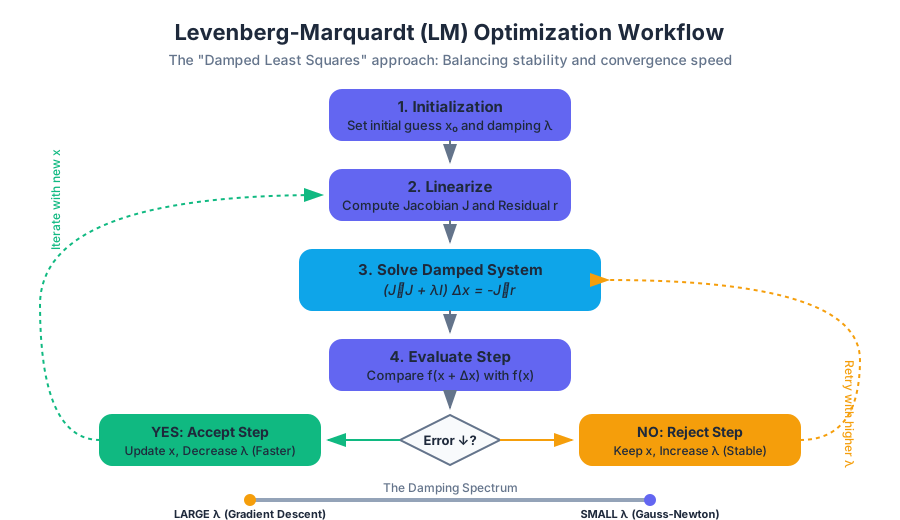
The LM update equation is: $$(J^T J + \lambda I) \Delta x = -J^T r$$ Where:
- If $\lambda$ is large, the term $\lambda I$ dominates. The step becomes $\Delta x \approx -\frac{1}{\lambda} J^T r$, which is a small step in the direction of the steepest descent.
- If $\lambda$ is small (approaching 0), the equation reverts to the Gauss-Newton update.
The Logic of $\lambda$ Adjustment:
The LM Logic: After calculating a step $\Delta x$, evaluate the new error $f(x_k + \Delta x)$.
- If the error decreased: Accept the step and decrease $\lambda$ (move closer to Gauss-Newton speed).
- If the error increased: Reject the step and increase $\lambda$ (move closer to Gradient Descent stability).
4. Comparison of Parameters
| Parameter | Effect of Increase | Effect of Decrease |
|---|---|---|
| Damping ($\lambda$) | More stable, smaller steps, Gradient Descent behavior | Faster convergence, larger steps, Gauss-Newton behavior |
| Jacobian ($J$) | Higher sensitivity to parameter changes | Lower sensitivity, potential for "flat" regions |
| Residual ($r$) | Indicates poor model fit or high noise | Indicates convergence or good model fit |
Constrained Nonlinear Least Squares
In many engineering contexts, parameters cannot take any value. They are subject to constraints (e.g., a physical length cannot be negative, or a probability must sum to one). We handle these using Penalty Algorithms and the Augmented Lagrangian.
Penalty Algorithms
A Penalty Method converts a constrained problem into an unconstrained one by adding a term to the objective function that "punishes" the violation of constraints.
Given the constraint $g(x) = 0$, we minimize: $$F(x, \rho) = \frac{1}{2} |r(x)|^2_2 + \frac{\rho}{2} |g(x)|^2_2$$ As the penalty parameter $\rho \to \infty$, the solution to the unconstrained problem converges to the solution of the constrained problem.
- Pros: Extremely simple to implement; works with standard NLS solvers.
- Cons: As $\rho$ becomes very large, the problem becomes ill-conditioned, making it nearly impossible for solvers like Gauss-Newton to find the minimum.
Augmented Lagrangian Method (ALM)
The Augmented Lagrangian is a more sophisticated approach that combines the Penalty method with Lagrange Multipliers. It overcomes the ill-conditioning of the simple penalty method.
The Augmented Lagrangian function is: $$\mathcal{L}_A(x, \lambda, \rho) = \frac{1}{2} |r(x)|^2_2 + \lambda^T g(x) + \frac{\rho}{2} |g(x)|^2_2$$ Where $\lambda$ is an estimate of the Lagrange multipliers.
The ALM Pipeline:
- Minimize $x$: Fix $\lambda_k$ and $\rho_k$, solve for $x$ using LM or GN.
- Update $\lambda$: $\lambda_{k+1} = \lambda_k + \rho_k g(x_{k+1})$.
- Update $\rho$: Increase $\rho$ if the constraint violation $g(x)$ isn't decreasing fast enough.
Key Insight: Unlike the penalty method, the Augmented Lagrangian does not require $\rho \to \infty$ to reach the exact solution. The inclusion of the $\lambda^T g(x)$ term "shifts" the objective so the minimum of the unconstrained function coincides with the constrained optimum even for finite $\rho$.
Implementation: Gauss-Newton in Python
The following code demonstrates a manual implementation of the Gauss-Newton algorithm to fit a nonlinear exponential decay model $y = a \cdot e^{bx}$ to noisy data.
import numpy as np

def model(x, params):
    """Nonlinear model: y = a * exp(b * x)"""
    a, b = params
    return a * np.exp(b * x)

def jacobian(x, params):
    """Jacobian matrix of the model with respect to [a, b]"""
    a, b = params
    # dr/da = exp(b*x)
    # dr/db = a * x * exp(b*x)
    da = np.exp(b * x)
    db = a * x * np.exp(b * x)
    return np.column_stack([da, db])

def gauss_newton(x_data, y_data, p0, iterations=10):
    p = np.array(p0, dtype=float)

    print(f"{'Iter':<5} | {'a':<10} | {'b':<10} | {'Cost':<10}")
    print("-" * 40)

    for i in range(iterations):
        # Calculate residuals
        r = y_data - model(x_data, p)
        cost = 0.5 * np.sum(r**2)

        # Calculate Jacobian
        J = jacobian(x_data, p)

        # Solve Normal Equations: (J^T J) * dp = J^T * r
        # Note: We use r = y - h(x), so dp = (J^T J)^-1 J^T r
        dp, _, _, _ = np.linalg.lstsq(J.T @ J, J.T @ r, rcond=None)

        # Update parameters
        p += dp

        print(f"{i:<5} | {p[0]:<10.4f} | {p[1]:<10.4f} | {cost:<10.4e}")

        if np.linalg.norm(dp) < 1e-6:
            break

    return p

# Generate synthetic data
x_true = np.linspace(0, 1, 20)
y_true = 2.5 * np.exp(-1.5 * x_true) + np.random.normal(0, 0.05, 20)

# Initial guess [a=1.0, b=-1.0]
final_params = gauss_newton(x_true, y_true, [1.0, -1.0])
Complexity and Performance Analysis
The computational bottleneck of NLS algorithms is typically the construction and inversion of the matrix $J^T J$.
| Operation | Complexity (Big O) | Notes |
|---|---|---|
| Jacobian Computation | $O(m \cdot n \cdot C)$ | $C$ is the cost of one partial derivative |
| Matrix Product ($J^T J$) | $O(m \cdot n^2)$ | Dominant term when $m \gg n$ |
| Matrix Inversion/Solve | $O(n^3)$ | Solved via Cholesky or QR factorization |
| Total per Iteration | $O(mn^2 + n^3)$ | Efficient for small $n$, even if $m$ is large |
Choosing the Right Algorithm
- Use Gauss-Newton if: You have a very good initial guess and the residuals at the solution are expected to be nearly zero (zero-residual problems).
- Use Levenberg-Marquardt if: You need a "workhorse" that is robust to poor initial guesses and handles ill-conditioned Jacobians. This is the default choice for most engineering applications.
- Use Penalty Methods if: You have simple constraints and a solver that can handle high-condition numbers.
- Use Augmented Lagrangian if: You need high precision for constrained problems and want to avoid the numerical instability of pure penalty methods.
Advanced Variations
1. Dogleg Method (Powell's Dogleg)
An alternative to LM, the Dogleg method is a Trust Region approach. It explicitly defines a region around $x_k$ where the linear model is trusted. It chooses a path that combines the Gauss-Newton step and the Steepest Descent step, staying strictly within the trust radius.
2. Robust Least Squares (M-Estimators)
In the presence of outliers, the squared error $|r(x)|^2$ is problematic because it gives too much weight to large residuals. Robust NLS replaces the square with a loss function $\rho(r_i)$, such as the Huber loss or the Cauchy loss, which "downweights" outliers.
3. Iteratively Reweighted Least Squares (IRLS)
IRLS is a technique to solve M-estimation problems by solving a sequence of weighted NLS problems. In each step, weights are calculated based on the residuals of the previous step: $$w_i = \frac{\psi(r_i)}{r_i}$$ where $\psi$ is the derivative of the robust loss function.
Summary of Key Connections
The evolution of these methods reflects a constant trade-off between convergence speed and robustness.
- Linear Least Squares is the "base case" where the surface is a perfect parabola.
- Gauss-Newton assumes the surface is "locally" a parabola and jumps to the bottom of that local approximation.
- Levenberg-Marquardt realizes the local parabola might be "flat" or "wrong" and adds a safety buffer (damping) to ensure we always move downhill.
- Augmented Lagrangian takes these unconstrained "downhill" walkers and gives them a way to respect walls and boundaries (constraints) without tripping over the numerical "stiffness" of those walls.
Source Materials
Study Applied Linear Algebra and Least Squares on Lykke
This course page is free to open: signed out, you can read its first two sections, and signing in, on any plan, opens the rest. The free Lykke Chrome extension syncs your own Canvas courses, so ChatGPT, Claude and Muse can answer from your classes and deadlines. It only reads Canvas.
Add the free extensionSign in to open every sectionAll sections of Applied Linear Algebra and Least Squares · Browse more course pages