From the free course Applied Linear Algebra and Least Squares on Lykke
Matrix Basics and Geometric Examples
Key concepts: Transpose · Matrix-vector multiplication · Incidence matrix · Convolution
Defines matrix dimensions, multiplication with vectors, and applications in geometry and graph theory.
Matrix Basics and Geometric Examples
In the landscape of applied linear algebra, a matrix is far more than a static rectangular grid of numbers. It is a linear operator—a mathematical machine that transforms vectors from one space to another. While a vector represents a point or a direction in $n$-dimensional space, a matrix represents a relationship between spaces. This section explores the fundamental mechanics of matrices, their geometric interpretations, and their specialized applications in graph theory and signal processing.
The Matrix as a Linear Operator
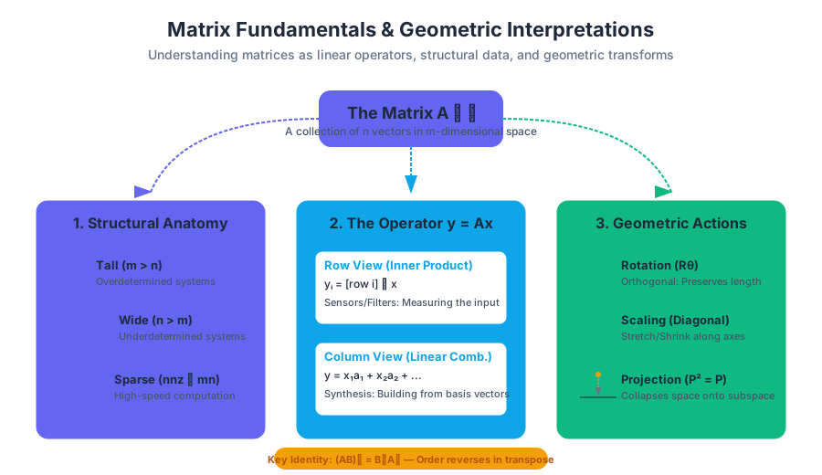
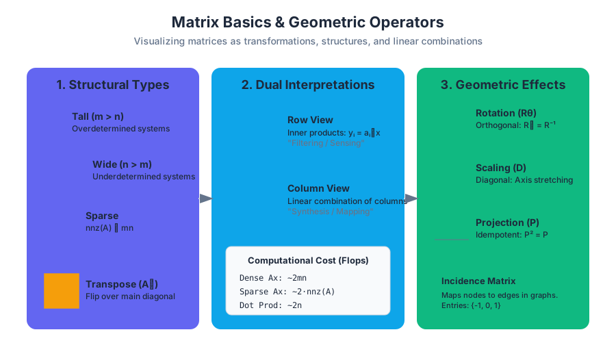
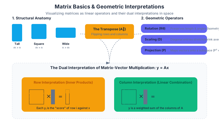
A matrix $A \in \mathbb{R}^{m \times n}$ consists of $m$ rows and $n$ columns. We refer to $m \times n$ as the dimensions of the matrix. If $m = n$, the matrix is square; if $m > n$, it is tall; and if $n > m$, it is wide.
Definition: A matrix $A$ is a collection of $n$ vectors $a_1, \dots, a_n \in \mathbb{R}^m$ arranged side-by-side: $$A = [a_1 \quad a_2 \quad \dots \quad a_n]$$ Alternatively, it can be viewed as a stack of $m$ row vectors.
Matrix Anatomy and Types
Understanding the structure of a matrix is the first step in determining the efficiency of the algorithms applied to it.
| Matrix Type | Condition | Significance |
|---|---|---|
| Square | $m = n$ | Represents transformations within the same dimensional space. |
| Tall | $m > n$ | Often represents overdetermined systems (more equations than variables). |
| Wide | $n > m$ | Often represents underdetermined systems (more variables than equations). |
| Sparse | $nnz(A) \ll mn$ | Most entries are zero; allows for specialized, high-speed computation. |
| Diagonal | $A_{ij} = 0$ for $i \neq j$ | Represents simple scaling along the axes. |
The Transpose Operation
The transpose of a matrix $A$, denoted $A^T$, is the matrix obtained by flipping $A$ over its main diagonal. Formally, $(A^T){ij} = A{ji}$.
Why it Matters
The transpose is not merely a reorientation of data; it is fundamental to the concept of duality. In optimization and physical systems, if $A$ represents a transformation from input to output, $A^T$ often represents the relationship between the sensitivities or forces in the reverse direction.
Mechanics and Properties
The transpose satisfies several algebraic identities that are essential for deriving complex linear models:
- $(A^T)^T = A$
- $(A + B)^T = A^T + B^T$
- $(\alpha A)^T = \alpha A^T$
- $(AB)^T = B^T A^T$ (Note the reversal of order)
Common Pitfalls
A frequent mistake is assuming that $A^T A = A A^T$. This is only true for normal matrices. For a tall matrix $A$, $A^T A$ is an $n \times n$ matrix (often the Gram matrix), while $A A^T$ is a much larger $m \times m$ matrix.
Matrix-Vector Multiplication
The operation $y = Ax$ is the cornerstone of linear algebra. It can be interpreted in two distinct, equally important ways.
1. The Row Interpretation (Inner Products)
In this view, each entry $y_i$ of the resulting vector is the inner product of the $i$-th row of $A$ with the vector $x$: $$y_i = \sum_{j=1}^n A_{ij} x_j$$ This perspective is useful when $A$ represents a set of sensors or filters, and $x$ is the input signal. Each $y_i$ is the "score" or "response" of the $i$-th filter to the input.
2. The Column Interpretation (Linear Combination)
This is the "geometric" view favored in modern data science. Here, $y$ is a linear combination of the columns of $A$, weighted by the entries of $x$: $$y = x_1 a_1 + x_2 a_2 + \dots + x_n a_n$$ This tells us that $y$ lies in the span of the columns of $A$. If $x$ is a vector of coefficients, $Ax$ is the process of synthesizing a new signal from the basis vectors stored in $A$.
Complexity and Performance
The computational cost of matrix-vector multiplication is a key constraint in large-scale systems.
| Operation | Flops (Floating Point Operations) |
|---|---|
| Inner product ($n$-vector) | $2n - 1$ |
| $Ax$ (where $A \in \mathbb{R}^{m \times n}$) | $\approx 2mn$ |
| $Ax$ (where $A$ is sparse) | $\approx 2 \cdot nnz(A)$ |
Geometric Transformations in 2D and 3D
Matrices act as geometric operators. By multiplying a vector (representing a point) by a specific matrix, we can rotate, scale, or project that point.
Scaling and Reflection
A diagonal matrix $D$ scales space along the principal axes. If $D = \text{diag}(2, 0.5)$, every $x$-coordinate doubles, and every $y$-coordinate is halved. Reflection across the $y$-axis is achieved by the matrix: $$ \text{Ref}_y = \begin{bmatrix} -1 & 0 \ 0 & 1 \end{bmatrix} $$
Rotation
To rotate a vector in $\mathbb{R}^2$ counter-clockwise by an angle $\theta$, we use the rotation matrix: $$ R_\theta = \begin{bmatrix} \cos \theta & -\sin \theta \ \sin \theta & \cos \theta \end{bmatrix} $$ This matrix is orthogonal, meaning $R_\theta^T = R_\theta^{-1}$, which implies that rotation preserves the length of vectors (isometry).
Projections
A projection matrix $P$ maps a vector onto a subspace. For example, projecting onto the $x$-axis in 2D: $$ P_x = \begin{bmatrix} 1 & 0 \ 0 & 0 \end{bmatrix} $$ Note that $P^2 = P$. Once you have projected a point onto a line, projecting it again changes nothing.
The Incidence Matrix
In graph theory and network analysis, the incidence matrix $A$ is a mathematical representation of a directed graph. It maps the relationship between $n$ nodes and $m$ edges.
Definition and Construction
For a graph with $n$ nodes and $m$ directed edges, the incidence matrix $A \in \mathbb{R}^{n \times m}$ is defined as:
- $A_{ij} = 1$ if edge $j$ enters node $i$.
- $A_{ij} = -1$ if edge $j$ leaves node $i$.
- $A_{ij} = 0$ otherwise.
Physical Interpretation: Flow and Potential
The incidence matrix is the bridge between local interactions (edges) and global states (nodes).
- Flow Conservation ($Ax = s$): If $x$ is a vector of flows on each edge, then $Ax$ is a vector where each entry $(Ax)_i$ represents the net flow out of node $i$. If $(Ax)_i = 0$, the node satisfies Kirchhoff's Current Law (flow in = flow out).
- Potential Difference ($v = A^T u$): If $u$ is a vector of potentials at each node (e.g., voltage or pressure), then $A^T u$ is a vector of potential differences across each edge.
Example: A Simple Triangle Graph
Consider a graph with 3 nodes and 3 edges forming a triangle:
- Edge 1: Node 1 $\to$ Node 2
- Edge 2: Node 2 $\to$ Node 3
- Edge 3: Node 3 $\to$ Node 1
The incidence matrix $A$ would be: $$ A = \begin{bmatrix} -1 & 0 & 1 \ 1 & -1 & 0 \ 0 & 1 & -1 \end{bmatrix} $$
| Feature | Interpretation in $Ax = b$ |
|---|---|
| Rows | Represent nodes; sum of row entries is always 0. |
| Columns | Represent edges; each column has exactly one $1$ and one $-1$. |
| Nullspace | The vector $\mathbf{1}$ (all ones) is always in the nullspace of $A^T$. |
Convolution as a Matrix Operation
Convolution is a fundamental operation in signal processing and deep learning. While often defined using a sliding window summation, it can be elegantly represented as a matrix-vector multiplication.
The Toeplitz Structure
When we convolve a signal $x$ with a filter $h$, we are essentially performing a weighted moving average. This can be written as $y = Hx$, where $H$ is a Toeplitz matrix. A Toeplitz matrix has the property that each descending diagonal from left to right is constant.
Example: 1D Moving Average
Suppose we have a 3-point moving average filter $h = [1/3, 1/3, 1/3]$. For an input signal $x \in \mathbb{R}^4$, the convolution (with zero padding) can be represented as: $$ \begin{bmatrix} y_1 \ y_2 \ y_3 \ y_4 \end{bmatrix} = \begin{bmatrix} 1/3 & 0 & 0 & 0 \ 1/3 & 1/3 & 0 & 0 \ 1/3 & 1/3 & 1/3 & 0 \ 0 & 1/3 & 1/3 & 1/3 \end{bmatrix} \begin{bmatrix} x_1 \ x_2 \ x_3 \ x_4 \end{bmatrix} $$
Why it Matters in Deep Learning
In Convolutional Neural Networks (CNNs), the "convolution" layer is actually a cross-correlation operation. However, the principle remains: the layer applies a sparse, weight-shared matrix to the input data. The sparsity and the Toeplitz-like structure allow CNNs to learn local features with far fewer parameters than a "fully connected" (dense) matrix.
Summary of Matrix Operations
To wrap up the basics, we compare the primary ways matrices interact with vectors and other matrices.
| Operation | Mathematical Form | Primary Application |
|---|---|---|
| Transformation | $y = Ax$ | Computer graphics, robotics, coordinate shifts. |
| System of Equations | $Ax = b$ | Solving for unknowns, engineering statics. |
| Change of Basis | $x = B\tilde{x}$ | Data compression (PCA), frequency analysis (DFT). |
| Graph Mapping | $b = Ax$ | Network flow, circuit analysis, logistics. |
| Filtering | $y = Hx$ | Audio processing, image blurring, trend extraction. |
Common Pitfalls in Matrix Basics
- Dimension Mismatch: The most common error in matrix-vector multiplication $Ax$ is attempting to multiply an $m \times n$ matrix by a vector of size $m$. The vector must be size $n$ (matching the number of columns).
- Non-Commutativity: In matrix-matrix multiplication, $AB \neq BA$ in general. Geometrically, this means the order of transformations matters—rotating then translating is not the same as translating then rotating.
- Interpreting Zero Net Flow: In incidence matrices, a net flow of zero at a node doesn't mean there is no activity; it means the system is in steady-state equilibrium.
- Transpose of a Product: Forgetting to reverse the order: $(AB)^T = B^T A^T$. This is vital when calculating gradients in machine learning (the "Backpropagation" rule).
Source Materials
Study Applied Linear Algebra and Least Squares on Lykke
This course page is free to open: signed out, you can read its first two sections, and signing in, on any plan, opens the rest. The free Lykke Chrome extension syncs your own Canvas courses, so ChatGPT, Claude and Muse can answer from your classes and deadlines. It only reads Canvas.
Add the free extensionSign in to open every sectionAll sections of Applied Linear Algebra and Least Squares · Browse more course pages