From the free course Applied Linear Algebra and Least Squares on Lykke
Matrix Multiplication and Inverses
Key concepts: Matrix multiplication · QR Factorization · Left and Right Inverses · Pseudo-inverse
Explains matrix-matrix multiplication, QR factorization, and the conditions for matrix invertibility.
Matrix Multiplication and Inverses
Overview
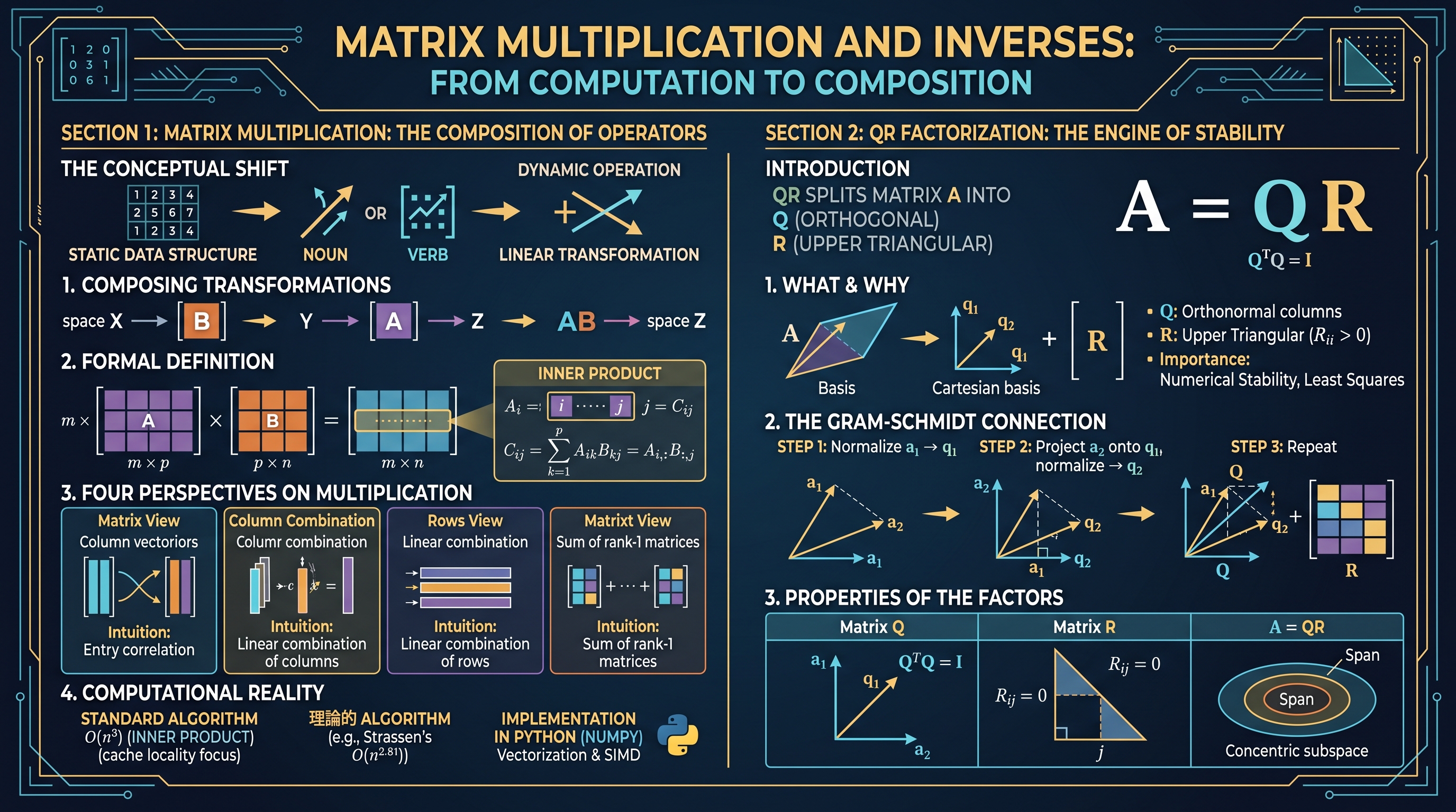
In the landscape of applied linear algebra, matrix multiplication and inversion represent the transition from static data structures to dynamic operations. While a vector might represent a state, a matrix represents a transformation—a "verb" that acts upon the "noun" of the vector. This section explores the mechanics of composing these transformations through multiplication and the sophisticated methods required to reverse them. We move beyond the elementary view of matrices as grids of numbers, treating them instead as operators, basis changes, and systems of linear equations.
Matrix Multiplication: The Composition of Operators
Matrix multiplication is the fundamental operation for composing linear transformations. If a matrix $B$ represents a transformation from space $\mathcal{X}$ to $\mathcal{Y}$, and a matrix $A$ represents a transformation from $\mathcal{Y}$ to $\mathcal{Z}$, then the product $C = AB$ represents the direct transformation from $\mathcal{X}$ to $\mathcal{Z}$.
1. Formal Definition
For an $m \times p$ matrix $A$ and a $p \times n$ matrix $B$, the product $C = AB$ is an $m \times n$ matrix. The entry in the $i$-th row and $j$-th column is defined as the inner product of the $i$-th row of $A$ and the $j$-th column of $B$:
Definition: Matrix-Matrix Product $$C_{ij} = \sum_{k=1}^{p} A_{ik}B_{kj} = A_{i,:} B_{:,j}$$ where $A_{i,:}$ is the $i$-th row of $A$ and $B_{:,j}$ is the $j$-th column of $B$.
2. Four Perspectives on Multiplication
To truly master matrix multiplication, one must be able to switch between different mental models of the operation:
| Perspective | Mathematical View | Intuition |
|---|---|---|
| Inner Product | $C_{ij} = \text{row}_i(A) \cdot \text{col}_j(B)$ | Each entry is a correlation between a row and a column. |
| Column Combination | $\text{col}_j(C) = A \cdot \text{col}_j(B)$ | Each column of $C$ is a linear combination of the columns of $A$. |
| Row Combination | $\text{row}_i(C) = \text{row}_i(A) \cdot B$ | Each row of $C$ is a linear combination of the rows of $B$. |
| Outer Product Sum | $C = \sum_{k=1}^{p} A_{:,k} B_{k,:}$ | $C$ is the sum of $p$ rank-1 matrices. |
3. Computational Complexity
The standard algorithm for multiplying an $m \times p$ matrix by a $p \times n$ matrix requires $m \cdot n \cdot p$ multiplications and $m \cdot n \cdot (p-1)$ additions. In asymptotic notation, for square $n \times n$ matrices, this is $O(n^3)$. While theoretical algorithms like Strassen's ($O(n^{2.81})$) exist, the "inner product" approach optimized for cache locality remains the standard in high-performance libraries like BLAS (Basic Linear Algebra Subprograms).
4. Implementation in Python (NumPy)
In modern engineering, we rarely implement the triple-nested loop. Instead, we use vectorized libraries that leverage SIMD instructions.
import numpy as np

# Define two matrices
A = np.array([[1, 2], [3, 4]])
B = np.array([[5, 6], [7, 8]])

# Matrix multiplication (Operator @ or np.matmul)
C = A @ B

# Verification of the Row-Column rule for C[0,0]
# C[0,0] = A[0,0]*B[0,0] + A[0,1]*B[1,0] = 1*5 + 2*7 = 19
print(f"Resulting Matrix C:\n{C}")
assert C[0,0] == 19
QR Factorization: The Engine of Stability
QR Factorization is the decomposition of a matrix $A$ into the product of an orthogonal matrix $Q$ and an upper triangular matrix $R$. It is the practical workhorse behind solving least squares problems and eigenvalue computations.
1. What it is
For an $m \times n$ matrix $A$ with linearly independent columns, the QR factorization is: $$A = QR$$
- $Q$ ($m \times n$): Has orthonormal columns ($Q^TQ = I$).
- $R$ ($n \times n$): An upper triangular matrix with positive diagonal entries ($R_{ii} > 0$).
2. Why it matters
Solving systems via the standard inverse is numerically risky. $R$, being triangular, allows for back-substitution, which is computationally efficient and stable. $Q$, being orthonormal, preserves lengths and angles, ensuring that rounding errors do not explode during computation.
3. The Gram-Schmidt Connection
The QR factorization is essentially the Gram-Schmidt orthogonalization process recorded in matrix form.
- Take the first column of $A$ ($a_1$) and normalize it to get $q_1$.
- Take the second column ($a_2$), subtract its projection onto $q_1$, and normalize the result to get $q_2$.
- Repeat for all $n$ columns.
- The coefficients used to "build" the original $a_i$ from the new $q_i$ form the matrix $R$.
4. Properties of the Factors
| Matrix | Property | Significance |
|---|---|---|
| $Q$ | $Q^T Q = I$ | $Q$ is a rigid transformation (rotation/reflection). |
| $R$ | $R_{ij} = 0$ for $i > j$ | Encapsulates the "dependency" structure of the columns. |
| $A=QR$ | $\text{span}(a_1 \dots a_k) = \text{span}(q_1 \dots q_k)$ | $Q$ provides an orthonormal basis for the same space. |
Matrix Inverses: Undoing Transformations
The inverse of a matrix $A$, denoted $A^{-1}$, is a matrix that "reverses" the effect of $A$. If $Ax = y$, then $x = A^{-1}y$.
1. The Square Case (Standard Inverse)
A square matrix $A$ has an inverse if and only if it is non-singular (its determinant is non-zero, or it has full rank).
- $AA^{-1} = I$
- $A^{-1}A = I$
2. Left and Right Inverses
In many real-world applications (like sensor fusion or over-determined control), matrices are not square. We then look for "one-sided" inverses.
3. Left Inverse (Tall Matrices)
If $A$ is $m \times n$ with $m > n$ (more equations than variables) and has full column rank, it has a left inverse $L$ such that $LA = I_n$.
- Formula: $L = (A^T A)^{-1} A^T$
- Application: This is the core of the Least Squares solution. It finds the $x$ that minimizes $|Ax - b|^2$.
4. Right Inverse (Wide Matrices)
If $A$ is $m \times n$ with $m < n$ (more variables than equations) and has full row rank, it has a right inverse $R$ such that $AR = I_m$.
- Formula: $R = A^T (AA^T)^{-1}$
- Application: This is used for Minimum Norm problems. Among all $x$ that satisfy $Ax = b$, the right inverse finds the one with the smallest magnitude ($|x|$).
| Inverse Type | Shape | Condition | Formula ($A^\dagger$) | Result |
|---|---|---|---|---|
| Standard | Square ($n \times n$) | Full Rank | $A^{-1}$ | $AA^{-1} = A^{-1}A = I$ |
| Left | Tall ($m \times n$) | Full Col Rank | $(A^T A)^{-1} A^T$ | $A^\dagger A = I$ |
| Right | Wide ($m \times n$) | Full Row Rank | $A^T (AA^T)^{-1}$ | $AA^\dagger = I$ |
The Pseudo-inverse (Moore-Penrose)
When a matrix is singular or not square, the Moore-Penrose Pseudo-inverse ($A^\dagger$) provides a generalized solution. It is the unique matrix that satisfies four criteria (the Moore-Penrose conditions), the most intuitive being that $AA^\dagger A = A$ and $A^\dagger A A^\dagger = A^\dagger$.
1. Computation via QR
Using the QR factorization $A = QR$, the pseudo-inverse (for a full-rank tall matrix) can be computed as: $$A^\dagger = R^{-1} Q^T$$ This is significantly more stable than calculating $(A^TA)^{-1}A^T$ directly, as forming $A^TA$ squares the condition number of the problem, potentially doubling the loss of precision.
2. Numerical Example
Consider a simple tall matrix: $$A = \begin{bmatrix} 1 \ 2 \end{bmatrix}$$ The left inverse is: $$A^\dagger = (A^T A)^{-1} A^T = ([1, 2] \begin{bmatrix} 1 \ 2 \end{bmatrix})^{-1} [1, 2] = (5)^{-1} [1, 2] = [0.2, 0.4]$$ Verification: $$A^\dagger A = [0.2, 0.4] \begin{bmatrix} 1 \ 2 \end{bmatrix} = 0.2(1) + 0.4(2) = 1$$
Common Pitfalls and Engineering Considerations
1. The "Never Invert" Rule
In numerical computing, there is a famous adage: "Never compute the inverse of a matrix explicitly."
- Why? Computing $A^{-1}$ is more expensive and less stable than solving the system $Ax = b$ using decompositions like QR or LU.
- Exception: When you need to update the solution for many different $b$ vectors very quickly and can tolerate slight precision loss, or in specific theoretical derivations.
2. Rank Deficiency
If a matrix does not have full rank, $(A^TA)$ or $(AA^T)$ will be non-invertible (singular).
- Symptom: A "Singular Matrix" error in code.
- Solution: Use the Singular Value Decomposition (SVD) to compute the pseudo-inverse, which handles rank deficiency by zeroing out the singular values below a certain threshold.
3. Non-Commutativity
A frequent mistake is assuming $AB = BA$. In the context of transformations, this is obvious: rotating a cube then sliding it is not the same as sliding it then rotating it.
- Algebraic Trap: $(AB)^{-1} = B^{-1}A^{-1}$. Note the reversal of order. This is the "Shoes and Socks" principle: to undo the process of putting on socks then shoes, you must first take off the shoes, then the socks.
4. Complexity Comparison
| Operation | Complexity | Notes |
|---|---|---|
| Matrix-Vector Mult | $O(n^2)$ | Highly parallelizable. |
| Matrix-Matrix Mult | $O(n^3)$ | The bottleneck of deep learning. |
| QR Factorization | $O(mn^2)$ | Stable, used for Least Squares. |
| Inversion (Square) | $O(n^3)$ | Generally avoided in favor of solve. |
Summary of Connections
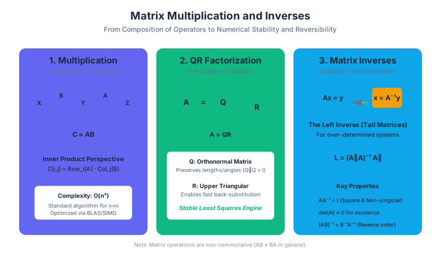
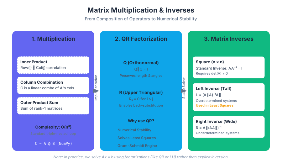
Matrix multiplication allows us to build complex models by stacking simpler ones. QR factorization provides the surgical precision needed to look inside those models and see which components are truly independent. Inverses and pseudo-inverses give us the power to work backward from observations to causes. Together, these tools form the mathematical backbone of everything from GPS positioning to the training of large language models.
Source Materials
Study Applied Linear Algebra and Least Squares on Lykke
This course page is free to open: signed out, you can read its first two sections, and signing in, on any plan, opens the rest. The free Lykke Chrome extension syncs your own Canvas courses, so ChatGPT, Claude and Muse can answer from your classes and deadlines. It only reads Canvas.
Add the free extensionSign in to open every sectionAll sections of Applied Linear Algebra and Least Squares · Browse more course pages