From the free course Applied Linear Algebra and Least Squares on Lykke
Linear Equations and Dynamical Systems
Key concepts: Affine functions · Systems of linear equations · State-space model · Population dynamics
Covers the representation of systems of equations and the modeling of time-varying states.
Linear Equations and Dynamical Systems
The transition from static vector operations to the study of Linear Equations and Dynamical Systems represents the shift from data representation to functional modeling. In this domain, we move beyond simply storing numbers in arrays to understanding how those numbers interact through transformations and how they evolve over time. By leveraging the structured properties of matrices, we can solve complex systems of constraints and predict the trajectory of physical, economic, and biological systems with high precision.
1. Affine and Linear Functions
At the core of linear modeling is the distinction between Linear Functions and Affine Functions. While often used interchangeably in casual conversation, their mathematical distinction is critical for accurate system modeling, particularly in data fitting and control theory.
What it is
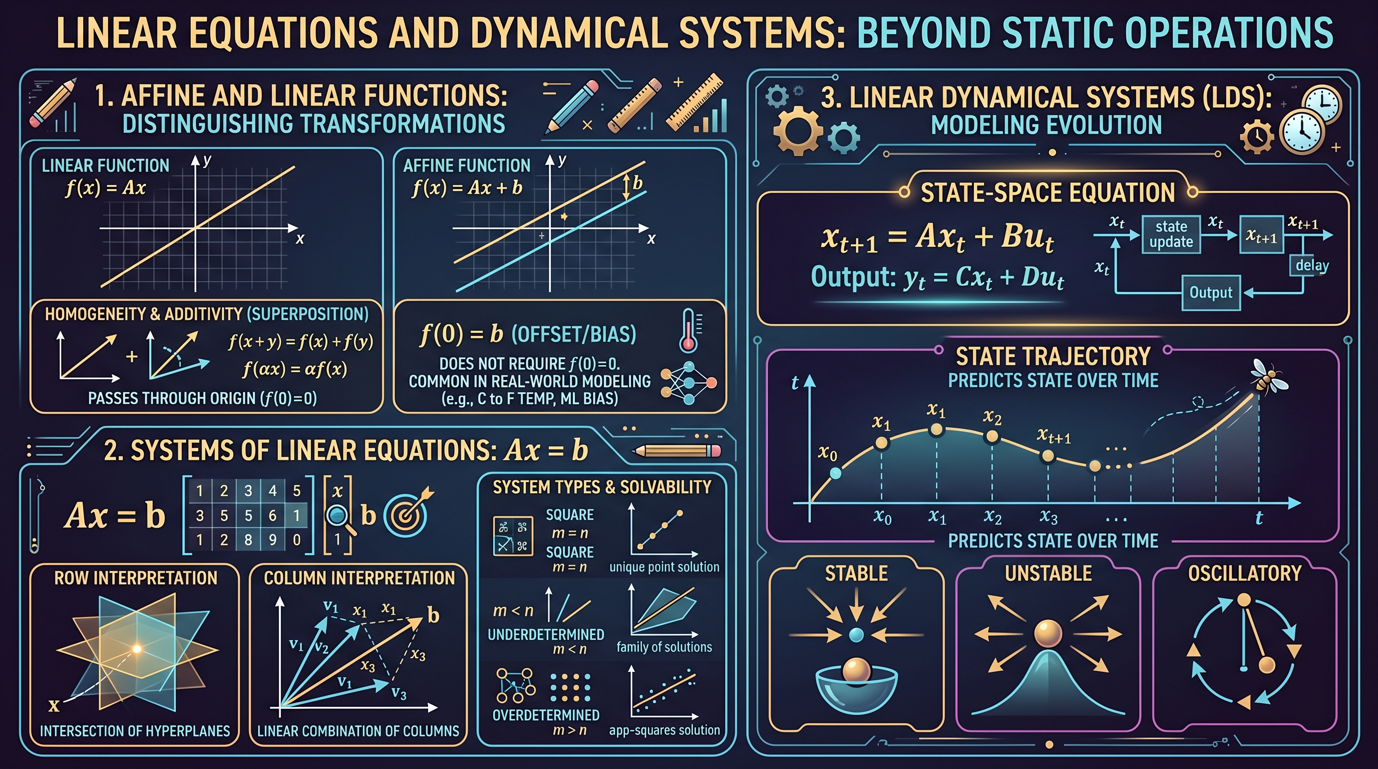
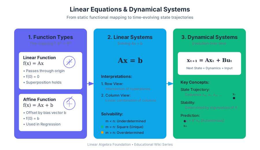
A function $f: \mathbb{R}^n \to \mathbb{R}^m$ is linear if it satisfies the properties of homogeneity and additivity (superposition). Mathematically, $f(x) = Ax$ for some matrix $A$. An affine function is a linear function plus a constant offset.
Definition: Affine Function A function $f: \mathbb{R}^n \to \mathbb{R}^m$ is affine if it can be expressed in the form: $$f(x) = Ax + b$$ where $A$ is an $m \times n$ matrix and $b$ is an $m$-vector (the offset or bias).
Why it matters
Most real-world relationships are not strictly linear; they do not pass through the origin $(0,0)$. For example, a temperature conversion from Celsius to Fahrenheit is affine ($F = 1.8C + 32$), not linear. In machine learning, the "weights" represent the linear transformation $A$, while the "bias" represents the affine offset $b$.
How it works
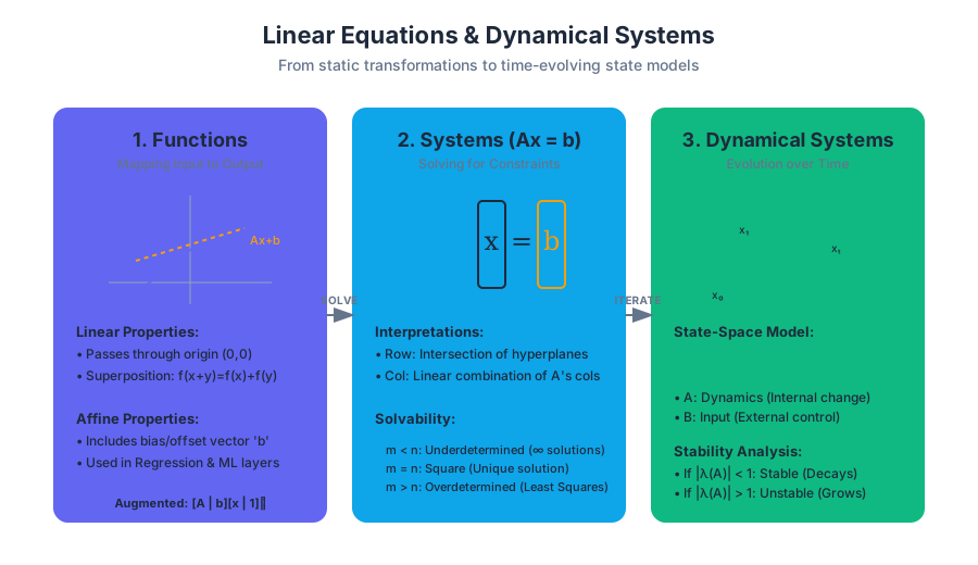
- Linearity Check: A function is linear if $f(0) = 0$. If $f(0) \neq 0$, the function is affine.
- Superposition: Linear functions satisfy $f(\alpha x + \beta y) = \alpha f(x) + \beta f(y)$. Affine functions do not satisfy this unless the sum of coefficients $\alpha + \beta = 1$.
- Matrix Representation: Any linear function can be represented as a matrix-vector product. To represent an affine function as a pure matrix-vector product, we often use augmented coordinates (adding a 1 to the vector $x$).
Comparison of Function Types
| Property | Linear Function ($Ax$) | Affine Function ($Ax + b$) |
|---|---|---|
| Passes through origin? | Yes ($f(0) = 0$) | No (unless $b=0$) |
| Superposition? | Always | Only if weights sum to 1 |
| Complexity (FLOPs) | $2mn$ | $2mn + m$ |
| Common Use Case | Physical scaling, rotations | Regression, Neural Network layers |
2. Systems of Linear Equations
A system of linear equations is a collection of $m$ equations involving $n$ variables. This is the "bread and butter" of applied linear algebra, represented compactly as $Ax = b$.
What it is
The equation $Ax = b$ represents a search for a vector $x$ that, when transformed by the matrix $A$, results in the vector $b$.
The Fundamental Problem Given $A \in \mathbb{R}^{m \times n}$ and $b \in \mathbb{R}^m$, find $x \in \mathbb{R}^n$ such that: $$ \sum_{j=1}^n A_{ij}x_j = b_i, \quad i = 1, \dots, m $$
Why it matters
Solving $Ax=b$ is the computational engine behind GPS positioning, structural engineering, circuit analysis, and economic equilibrium models. It allows us to reverse-engineer a cause ($x$) from an effect ($b$) given a known mechanism ($A$).
Interpretations of $Ax = b$
- Row Interpretation: Each row of $A$ represents a hyperplane in $n$-dimensional space. The solution $x$ is the intersection point of all these hyperplanes.
- Column Interpretation: $Ax$ is a linear combination of the columns of $A$. We are looking for the weights $x_1, \dots, x_n$ that combine the columns to produce $b$.
Solvability and System Types
| System Type | Relation | Interpretation | Typical Outcome |
|---|---|---|---|
| Square | $m = n$ | Same number of equations and unknowns | Unique solution (usually) |
| Underdetermined | $m < n$ | More unknowns than equations | Infinitely many solutions |
| Overdetermined | $m > n$ | More equations than unknowns | No exact solution (requires Least Squares) |
Common Pitfalls
- Singularity: A square matrix $A$ might not have a solution if its columns are linearly dependent (the matrix is "singular").
- Ill-conditioning: Small changes in $b$ can lead to massive changes in $x$ if the matrix $A$ is nearly singular, leading to numerical instability.
3. Linear Dynamical Systems (LDS)
A Linear Dynamical System describes how a state vector $x$ evolves over discrete time steps. It is the primary tool for modeling systems that change, from the cooling of a coffee cup to the fluctuations of the stock market.
What it is
An LDS is defined by a state-space equation where the next state is a linear function of the current state.
State-Space Model (Discrete Time) $$x_{t+1} = Ax_t + Bu_t$$ Where:
- $x_t$: State vector at time $t$ (the "memory" of the system).
- $A$: Dynamics matrix (describes internal evolution).
- $u_t$: Input vector (external forces or control signals).
- $B$: Input matrix (how external forces affect the state).
Why it matters
Dynamical systems allow for prediction and control. If we know the current state $x_0$ and the dynamics $A$, we can predict the state at any future time $T$ by calculating $x_T = A^T x_0$.
How it works: The Trajectory
The sequence of states $x_0, x_1, x_2, \dots$ is called the trajectory of the system.
- Autonomous Systems: If there are no inputs ($u_t = 0$), the system is $x_{t+1} = Ax_t$.
- Evolution: The state at time $t$ is $x_t = A^t x_0$.
- Stability:
- If the eigenvalues of $A$ are all less than 1 in magnitude, the system is stable ($x_t \to 0$).
- If any eigenvalue is greater than 1, the system explodes ($x_t \to \infty$).
Components of a State-Space Model
| Component | Symbol | Role |
|---|---|---|
| State | $x_t$ | Minimum information needed to predict the future. |
| Dynamics Matrix | $A$ | Determines the "physics" or "rules" of the system. |
| Input | $u_t$ | External control (e.g., accelerator pedal, medicine dosage). |
| Output | $y_t$ | What we actually observe (often $y_t = Cx_t$). |
4. Population Dynamics: A Concrete Case Study
One of the most intuitive applications of LDS is Population Dynamics, specifically using the Leslie Matrix model to track age-structured populations.
The Scenario
Imagine a population of animals divided into three age groups: Young, Juvenile, and Adult. We want to model how this population changes every year.
The Mechanics
The state vector is $x_t = [x_{1,t}, x_{2,t}, x_{3,t}]^T$, representing the number of individuals in each group. The dynamics are governed by:
- Birth rates ($b_i$): How many offspring each group produces.
- Survival rates ($s_i$): The probability of moving to the next age group.
The matrix $A$ (Leslie Matrix) looks like this: $$ A = \begin{bmatrix} b_1 & b_2 & b_3 \ s_1 & 0 & 0 \ 0 & s_2 & 0 \end{bmatrix} $$
Worked Example
Suppose:
- Birth rates: $b_1=0, b_2=0.5, b_3=2.0$
- Survival rates: $s_1=0.8, s_2=0.5$
- Initial population: $x_0 = [100, 50, 20]^T$
Step 1: Calculate $x_1$ $$ x_1 = Ax_0 = \begin{bmatrix} 0 & 0.5 & 2.0 \ 0.8 & 0 & 0 \ 0 & 0.5 & 0 \end{bmatrix} \begin{bmatrix} 100 \ 50 \ 20 \end{bmatrix} = \begin{bmatrix} (0.5 \times 50) + (2 \times 20) \ 0.8 \times 100 \ 0.5 \times 50 \end{bmatrix} = \begin{bmatrix} 65 \ 80 \ 25 \end{bmatrix} $$
Step 2: Analysis The total population changed from 170 to 170. However, the distribution shifted. Over many iterations, the population will either stabilize to a specific age distribution or grow/shrink exponentially depending on the dominant eigenvalue of $A$.
Population Dynamics Parameters
| Parameter | Symbol | Impact on System |
|---|---|---|
| Fecundity | $b_i$ | Increases the first entry of $x_{t+1}$ (births). |
| Survivorship | $s_i$ | Shifts population from $x_i$ to $x_{i+1}$. |
| Growth Factor | $\lambda$ | The rate at which the total population scales per step. |
5. Computational Complexity and FLOPs
Understanding the cost of these operations is vital for large-scale engineering.
Matrix-Vector Multiplication
To compute $y = Ax$ where $A \in \mathbb{R}^{m \times n}$:
- Each of the $m$ rows requires $n$ multiplications and $n-1$ additions.
- Total FLOPs (Floating Point Operations) $\approx 2mn$.
Dynamical System Simulation
To simulate $T$ steps of an autonomous LDS $x_{t+1} = Ax_t$:
- Each step is one matrix-vector multiply ($2n^2$ flops).
- Total complexity: $O(T \cdot n^2)$.
Insight: Sparsity In many real-world systems (like power grids or social networks), the matrix $A$ is sparse (mostly zeros). If $A$ has only $nnz$ non-zero entries, the complexity drops to $O(T \cdot nnz)$, which is significantly faster.
6. Summary of Extensions
Linear equations and dynamical systems serve as the foundation for more advanced topics:
- Least Squares: When $Ax=b$ has no solution (overdetermined), we find $x$ that minimizes $|Ax - b|^2$.
- Control Theory: Finding a sequence of inputs $u_0, u_1, \dots$ to drive the state $x_T$ to a desired target.
- Markov Chains: A special case of LDS where $x_t$ represents probabilities and the columns of $A$ sum to 1.
- Linear Regression: An affine modeling problem where we solve for the matrix $A$ and bias $b$ given observed data.
Study Guide: Linear Equations and Dynamical Systems
1. Core Definitions
- Linear Function: $f(x) = Ax$. Must satisfy $f(0)=0$ and superposition.
- Affine Function: $f(x) = Ax + b$. A linear transformation plus a translation.
- State Vector ($x_t$): A vector representing the condition of a system at time $t$.
- Dynamics Matrix ($A$): A square matrix defining how the state transitions from $t$ to $t+1$.
2. Solving $Ax=b$
- If $A$ is invertible, $x = A^{-1}b$.
- If $A$ is overdetermined, use the Normal Equations: $x = (A^T A)^{-1} A^T b$.
- If $A$ is underdetermined, there are infinitely many solutions; we often seek the one with the minimum norm.
3. Dynamical System Properties
- Autonomous: $x_{t+1} = Ax_t$.
- Input-Driven: $x_{t+1} = Ax_t + Bu_t$.
- Stability: Determined by the eigenvalues of $A$. If $\max|\lambda_i| < 1$, the system is stable.
- Leslie Matrix: A specific LDS used in biology to model age-structured population growth.
4. Computational Efficiency
- Matrix-vector multiplication: $2mn$ flops.
- Sparse matrices significantly reduce the cost of simulating high-dimensional dynamical systems.
- Solving $Ax=b$ via Gaussian elimination or QR factorization typically costs $O(n^3)$ for an $n \times n$ matrix.
5. Common Pitfalls to Avoid
- Confusing linear and affine functions in models where the offset $b$ is non-zero.
- Ignoring the "curse of dimensionality" when the state vector $x$ becomes extremely large.
- Assuming a system is stable without checking the properties of the dynamics matrix $A$.
Source Materials
Study Applied Linear Algebra and Least Squares on Lykke
This course page is free to open: signed out, you can read its first two sections, and signing in, on any plan, opens the rest. The free Lykke Chrome extension syncs your own Canvas courses, so ChatGPT, Claude and Muse can answer from your classes and deadlines. It only reads Canvas.
Add the free extensionSign in to open every sectionAll sections of Applied Linear Algebra and Least Squares · Browse more course pages