From the free course Applied Linear Algebra and Least Squares on Lykke
The Least Squares Problem and Data Fitting
Key concepts: Residual norm · Normal equations · Feature engineering · Overfitting · Least squares classifier
Focuses on minimizing the residual norm and applying least squares to regression and classification.
The Least Squares Problem and Data Fitting
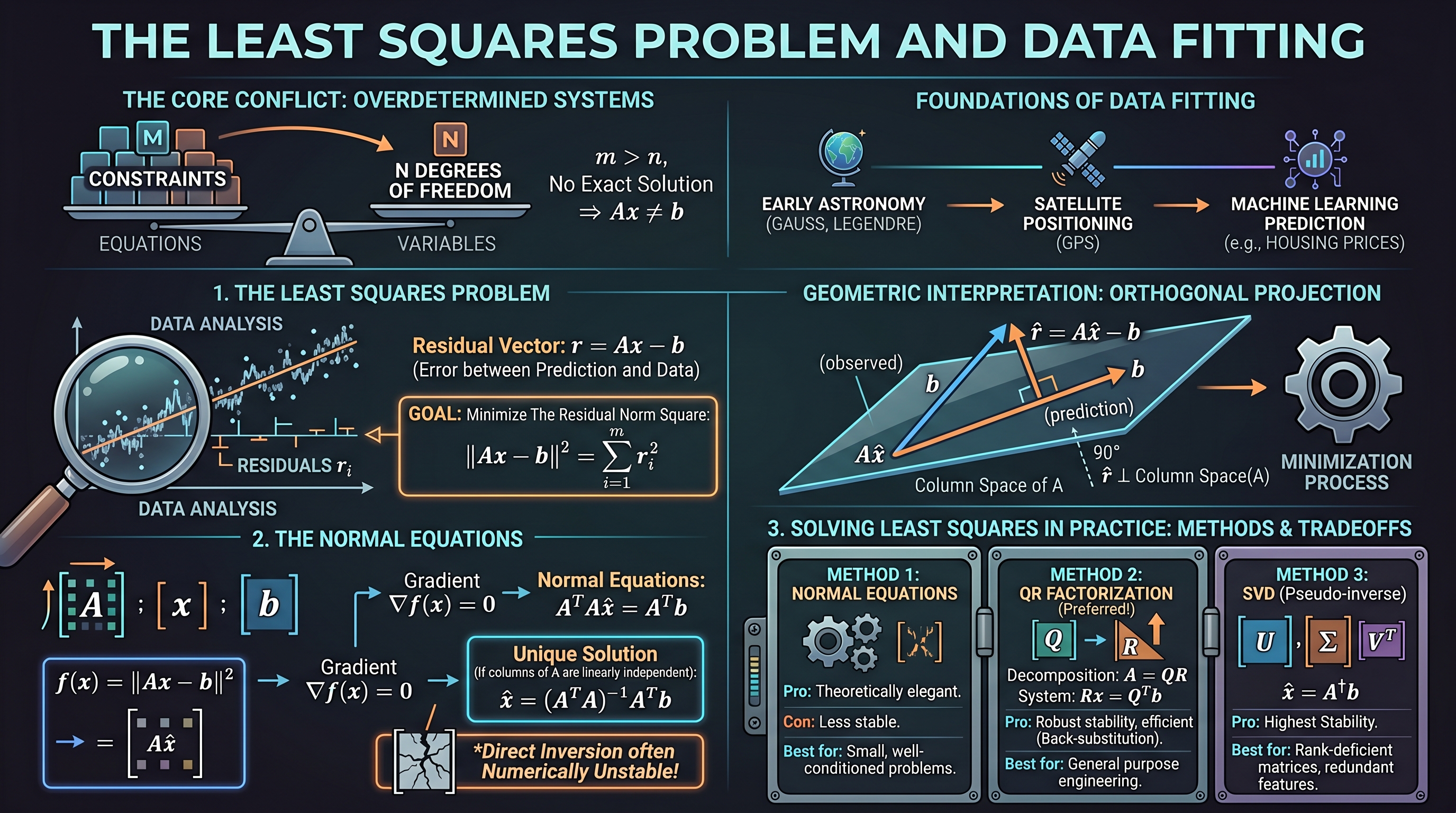
In the landscape of applied mathematics and engineering, few tools are as ubiquitous or as foundational as the Least Squares method. At its core, the least squares problem addresses a fundamental conflict: how do we "solve" a system of linear equations when no exact solution exists? This situation, known as an overdetermined system, occurs whenever we have more constraints (equations) than degrees of freedom (variables).
Whether it is a satellite determining its position from noisy GPS signals, a machine learning model predicting housing prices, or a control system stabilizing an aircraft, least squares provides the mathematical framework for finding the "best fit" solution by minimizing the discrepancy between observation and prediction.
1. The Least Squares Problem
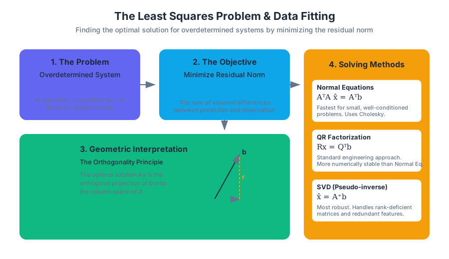
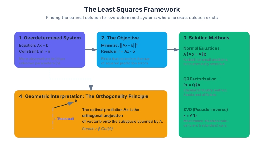
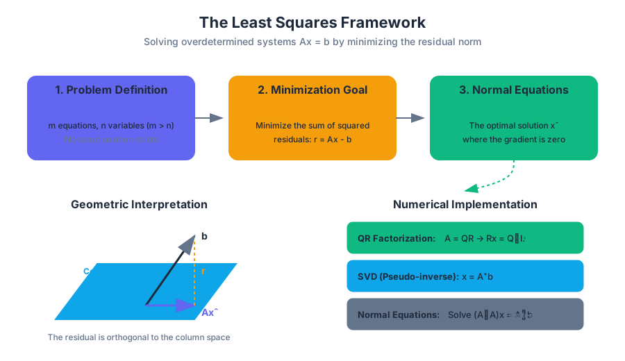
The least squares problem is defined by an overdetermined system of linear equations $Ax = b$, where $A$ is an $m \times n$ matrix with $m > n$. In such cases, the vector $b$ is typically not in the range (column space) of $A$, meaning there is no $x$ such that $Ax$ exactly equals $b$.
1.1 The Residual Norm
To find the best approximation, we define the residual vector $r$, which represents the error between our prediction $Ax$ and the actual data $b$:
Definition: Residual Vector For a given $x$, the residual $r$ is defined as: $$r = Ax - b$$ The "size" of this error is measured using the Euclidean norm (or $L_2$ norm), and the goal of least squares is to find the $x$ that minimizes the square of this norm: $$\text{minimize } |Ax - b|^2 = \sum_{i=1}^m (a_i^T x - b_i)^2$$
By squaring the norm, we ensure the objective function is differentiable and penalize larger errors more heavily than smaller ones.
1.2 The Objective Function
The function $f(x) = |Ax - b|^2$ is a convex quadratic function. Because it is convex, any local minimum is also a global minimum. The point $\hat{x}$ that minimizes this function is called the least squares solution.
| Component | Symbol | Dimension | Description |
|---|---|---|---|
| Feature Matrix | $A$ | $m \times n$ | The data matrix containing $m$ observations and $n$ features. |
| Parameter Vector | $x$ | $n \times 1$ | The unknown coefficients we seek to estimate. |
| Target Vector | $b$ | $m \times 1$ | The observed outcomes or measurements. |
| Residual | $r$ | $m \times 1$ | The difference $Ax - b$; the "unexplained" part of the data. |
| Residual Norm | $|r|$ | Scalar | The total magnitude of error. |
2. The Normal Equations
To find the minimum of $|Ax - b|^2$, we can use multivariable calculus. By setting the gradient of the objective function with respect to $x$ to zero, we derive the Normal Equations.
2.1 Derivation and Mechanics
Expanding the squared norm gives: $$|Ax - b|^2 = (Ax - b)^T(Ax - b) = x^T A^T A x - 2b^T A x + b^T b$$
Taking the derivative with respect to $x$ and setting it to zero results in: $$2A^T A x - 2A^T b = 0$$ Which simplifies to the standard form of the normal equations:
The Normal Equations $$A^T A \hat{x} = A^T b$$ If the columns of $A$ are linearly independent, then the matrix $A^T A$ (the Gram matrix) is invertible, and the unique solution is: $$\hat{x} = (A^T A)^{-1} A^T b$$
2.2 Geometric Interpretation: The Orthogonality Principle
Geometrically, the least squares solution $\hat{x}$ has a profound property: the optimal residual vector $\hat{r} = A\hat{x} - b$ is orthogonal to the column space of $A$. This means that the error is perpendicular to every feature vector in our model. In other words, $A\hat{x}$ is the orthogonal projection of $b$ onto the subspace spanned by the columns of $A$.
3. Solving Least Squares in Practice
While the formula $\hat{x} = (A^T A)^{-1} A^T b$ is theoretically elegant, it is often numerically unstable to compute $(A^T A)^{-1}$ directly, especially if $A$ is "ill-conditioned" (meaning some columns are nearly linearly dependent).
3.1 QR Factorization
The preferred method for solving least squares in modern software is QR Factorization. We decompose $A$ into an $m \times n$ matrix $Q$ with orthonormal columns and an $n \times n$ upper triangular matrix $R$: $$A = QR$$
Substituting this into the normal equations: $$(QR)^T (QR) x = (QR)^T b$$ $$R^T Q^T Q R x = R^T Q^T b$$ Since $Q^T Q = I$ (identity matrix) and $R$ is invertible: $$R x = Q^T b$$
This system can be solved efficiently using back-substitution because $R$ is upper triangular.
| Method | Complexity (Flops) | Stability | Best For |
|---|---|---|---|
| Normal Equations | $n^2 m + \frac{1}{3}n^3$ | Lower | Small, well-conditioned problems. |
| QR Factorization | $2n^2 m - \frac{2}{3}n^3$ | High | General purpose, robust engineering. |
| SVD (Pseudo-inverse) | $O(mn^2)$ | Highest | Rank-deficient matrices (redundant features). |
import numpy as np

# Example: Solving Least Squares using NumPy
# A is 100x3 (100 observations, 3 features)
# b is 100x1 (100 targets)
A = np.random.randn(100, 3)
b = np.random.randn(100)

# Method 1: Direct solver (uses QR or SVD internally)
x_hat, residuals, rank, s = np.linalg.lstsq(A, b, rcond=None)

# Method 2: Manual Normal Equations (Not recommended for production)
x_normal = np.linalg.inv(A.T @ A) @ A.T @ b

print(f"Least Squares Coefficients: {x_hat}")
4. Data Fitting and Feature Engineering
Least squares is the engine behind Data Fitting, where we attempt to find a mathematical function $f(u)$ that maps an input $u$ to an output $y$.
4.1 From Linear to Non-linear Fitting
Even though the method is called "linear" least squares, it can fit highly non-linear relationships. The "linear" refers to the parameters $x$, not the input data $u$. We achieve this through feature engineering—transforming the raw input $u$ into a vector of features $a = \phi(u)$.
The model takes the form: $$y \approx x_1 \phi_1(u) + x_2 \phi_2(u) + \dots + x_n \phi_n(u)$$
4.2 Common Basis Functions
To fit complex data, we choose a set of basis functions that we believe represent the underlying physical or statistical process.
| Basis Type | Transformation $\phi(u)$ | Application |
|---|---|---|
| Linear | $[1, u]$ | Simple trend lines. |
| Polynomial | $[1, u, u^2, \dots, u^p]$ | Curves, non-linear growth. |
| Sinusoidal | $[\sin(u), \cos(u)]$ | Seasonal data, periodic signals. |
| Logarithmic | $[\log(u)]$ | Diminishing returns, saturation effects. |
| Radial Basis | $\exp(-|u - c|^2 / \sigma^2)$ | Localized fitting, non-parametric shapes. |
5. Overfitting and Validation
A common pitfall in data fitting is overfitting. This occurs when a model is so complex (e.g., a high-degree polynomial) that it fits the noise in the training data rather than the underlying pattern.
5.1 The Training vs. Test Split
To detect overfitting, we never evaluate a model solely on the data used to train it. Instead, we split our data into two or three sets:
- Training Set: Used to solve the least squares problem and find $\hat{x}$.
- Validation Set: Used to choose "hyperparameters," such as the degree of the polynomial or the number of features.
- Test Set: Used for a final, unbiased evaluation of the model's performance on unseen data.
5.2 Generalization Error
If the residual norm on the training set is very low, but the residual norm on the test set is very high, the model has failed to generalize.
Key Insight: The Complexity Tradeoff As model complexity (number of features $n$) increases:
- Training Error always decreases (or stays the same).
- Test Error initially decreases but eventually starts to increase as the model begins to "memorize" noise.
| Metric | Training Error | Test Error | Interpretation |
|---|---|---|---|
| High / High | High | High | Underfitting: Model is too simple. |
| Low / High | Low | High | Overfitting: Model is too complex/noisy. |
| Low / Low | Low | Low | Good Fit: Model has captured the pattern. |
6. The Least Squares Classifier
While least squares is primarily a regression tool (predicting continuous numbers), it can be adapted for classification (predicting categories).
6.1 Binary Classification
Suppose we want to classify data into two groups, labeled $+1$ and $-1$. We can fit a linear function $f(u) = a^T x + b$ such that:
- $f(u) \approx +1$ for class 1
- $f(u) \approx -1$ for class 2
To classify a new point $u$, we simply look at the sign of the prediction: $$\hat{y} = \text{sign}(a^T \hat{x} + \hat{b})$$
6.2 The Decision Boundary
The set of points where $a^T \hat{x} + \hat{b} = 0$ defines the decision boundary. For a 2D input, this is a line; for 3D, a plane; and for higher dimensions, a hyperplane. Points on one side are classified as positive, and points on the other as negative.
6.3 Multi-class Classification (One-vs-All)
To classify data into $K$ classes, we can train $K$ separate least squares classifiers. For each class $k$, we create a target vector $b^{(k)}$ where $b_i = 1$ if observation $i$ belongs to class $k$, and $b_i = -1$ otherwise. To classify a new point, we run it through all $K$ models and choose the class that yields the highest (most positive) value.
7. Common Pitfalls and Best Practices
- Ignoring the Intercept: Always include a "ones" column in your matrix $A$ (unless your data is centered). Without it, your model is forced to pass through the origin $(0,0)$, which rarely fits real-world data.
- Multi-collinearity: If two features are highly correlated (e.g., height in inches and height in centimeters), the matrix $A^T A$ becomes nearly singular. This leads to massive, unstable values in $\hat{x}$.
- Outliers: Because least squares minimizes the squared error, a single outlier (a data point very far from the rest) can pull the entire model toward it, ruining the fit for the majority of the data. In such cases, robust regression or $L_1$ minimization might be preferred.
- Feature Scaling: While theoretically not required for the basic least squares solution, scaling features to have similar ranges (e.g., between 0 and 1) is crucial for numerical stability and when adding regularization.
Summary of the Least Squares Pipeline
- Data Collection: Gather $m$ pairs of inputs $u_i$ and outputs $y_i$.
- Feature Engineering: Choose basis functions $\phi(u)$ to form the feature matrix $A$.
- Partitioning: Split data into training and test sets.
- Optimization: Solve $A^T A \hat{x} = A^T b$ using QR factorization on the training set.
- Validation: Evaluate the residual norm on the test set.
- Iteration: Adjust features or model complexity if the test error is too high.
Source Materials
Study Applied Linear Algebra and Least Squares on Lykke
This course page is free to open: signed out, you can read its first two sections, and signing in, on any plan, opens the rest. The free Lykke Chrome extension syncs your own Canvas courses, so ChatGPT, Claude and Muse can answer from your classes and deadlines. It only reads Canvas.
Add the free extensionSign in to open every sectionAll sections of Applied Linear Algebra and Least Squares · Browse more course pages