From the free course Applied Linear Algebra and Least Squares on Lykke
Regularization and Constrained Least Squares
Key concepts: Tikhonov regularization · Trade-off curves · KKT equations · Constrained least squares
Covers Tikhonov regularization for stability and solving least squares with equality constraints.
Regularization and Constrained Least Squares
In the pursuit of fitting models to data, the standard least squares approach—minimizing the sum of squared residuals—is often insufficient. While it provides the "best fit" in a purely algebraic sense, it frequently fails in the face of noisy data, collinear features, or physical requirements that the solution must satisfy. To address these challenges, we turn to Regularization and Constrained Least Squares. These techniques allow us to incorporate prior knowledge, ensure numerical stability, and manage the fundamental trade-off between model complexity and accuracy.
Tikhonov Regularization
Standard least squares seeks to minimize $|Ax - b|^2$. However, when the matrix $A$ is ill-conditioned (i.e., its columns are nearly linearly dependent) or when the number of parameters exceeds the number of observations, the resulting solution $x$ can have extremely large magnitudes. This phenomenon, often called "overfitting," results in a model that captures noise rather than the underlying signal.
Tikhonov regularization, also known as Ridge Regression or $L_2$ Regularization, addresses this by adding a penalty term to the objective function.
1. What it is
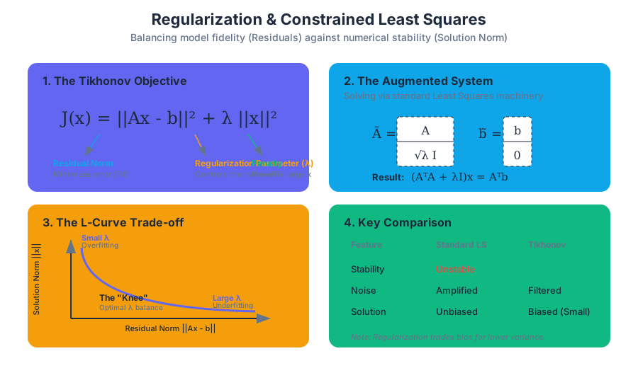
Tikhonov regularization modifies the least squares objective to include a weighted penalty on the norm of the solution vector $x$. The regularized objective function $J(x)$ is defined as:
Definition: Tikhonov Regularized Objective $$J(x) = |Ax - b|^2 + \lambda |x - x_{prior}|^2$$ Where $\lambda > 0$ is the regularization parameter and $x_{prior}$ is a suggested or "default" value for $x$ (often the zero vector).
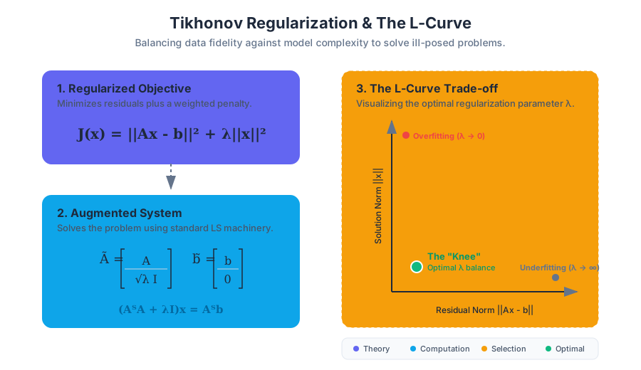
In the most common case where $x_{prior} = 0$, the objective becomes: $$J(x) = |Ax - b|^2 + \lambda |x|^2$$
2. Why it matters
Regularization is the primary tool for solving ill-posed problems. It provides several critical benefits:
- Numerical Stability: It ensures that the matrix $(A^TA + \lambda I)$ is invertible, even if $A^TA$ is singular.
- Generalization: By penalizing large coefficients, it prevents the model from "chasing noise," leading to better performance on unseen data.
- Preference Incorporation: It allows the user to specify that the solution should be "small" or "smooth," which is a common physical or logical requirement.
3. How it works: The Augmented Matrix
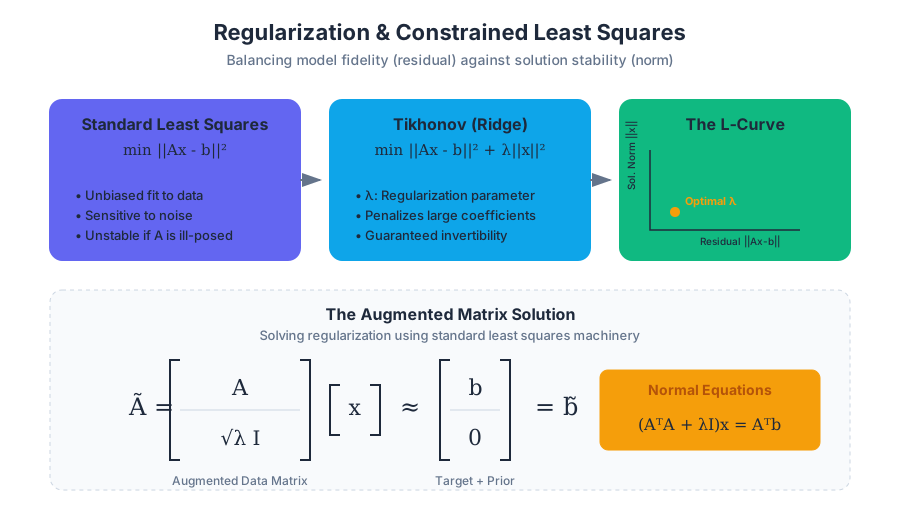
One of the most elegant aspects of Tikhonov regularization is that it can be solved using the standard least squares machinery. We can reformulate the regularized problem as an augmented least squares problem.
To minimize $|Ax - b|^2 + \lambda |x|^2$, we define an augmented matrix $\tilde{A}$ and an augmented vector $\tilde{b}$: $$\tilde{A} = \begin{bmatrix} A \ \sqrt{\lambda}I \end{bmatrix}, \quad \tilde{b} = \begin{bmatrix} b \ 0 \end{bmatrix}$$
The problem then becomes minimizing $|\tilde{A}x - \tilde{b}|^2$. The normal equations for this augmented system are: $$(A^TA + \lambda I)x = A^Tb$$
| Feature | Standard Least Squares | Tikhonov Regularization |
|---|---|---|
| Objective | Minimize $|Ax - b|^2$ | Minimize $|Ax - b|^2 + \lambda |x|^2$ |
| Normal Equations | $A^TAx = A^Tb$ | $(A^TA + \lambda I)x = A^Tb$ |
| Invertibility | Requires $A$ to have full column rank | Guaranteed for any $\lambda > 0$ |
| Solution Norm | Can be very large | Controlled by $\lambda$ |
| Sensitivity to Noise | High | Low (Filtered) |
4. Concrete Example: Polynomial Interpolation
Imagine fitting a 10th-degree polynomial to 5 data points. A standard least squares fit will pass through every point perfectly but will oscillate wildly between them. By applying Tikhonov regularization with a small $\lambda$, we penalize the magnitude of the polynomial coefficients. This "flattens" the oscillations, resulting in a curve that captures the general trend of the data without over-fitting the specific noise in the 5 points.
5. Common Pitfalls
- Scaling Matters: Because the penalty $\lambda |x|^2$ treats all components of $x$ equally, it is crucial to scale the features (columns of $A$) so they have similar magnitudes. If one feature is measured in millimeters and another in kilometers, the regularization will disproportionately affect the one with the smaller numerical values.
- Bias-Variance Trade-off: Regularization introduces bias (the solution is no longer the "unbiased" minimum of the residuals) to reduce variance (sensitivity to the specific data sample). Choosing $\lambda$ too high will lead to "underfitting," where the model is too simple to capture the signal.
Trade-off Curves and the Pareto Frontier
The choice of the regularization parameter $\lambda$ is the central challenge in regularized least squares. It represents a fundamental trade-off between two competing goals: minimizing the residual norm (fit to data) and minimizing the solution norm (model complexity).
1. The Concept of Pareto Optimality
For any given $\lambda$, the resulting solution $x_\lambda$ is Pareto optimal. This means you cannot improve the fit (decrease $|Ax - b|$) without increasing the complexity (increasing $|x|$), and vice versa.
2. The L-Curve
When we plot the residual norm $|Ax_\lambda - b|$ against the solution norm $|x_\lambda|$ for a wide range of $\lambda$ values, we typically see an L-shaped curve.
- The Horizontal Part: Large $\lambda$. The solution norm is small, but the residual is very sensitive to changes in $\lambda$.
- The Vertical Part: Small $\lambda$. The residual is small, but the solution norm explodes as we try to fit the noise.
- The "Knee": The point of maximum curvature. This is often considered the "optimal" $\lambda$ as it balances both objectives effectively.
3. Parameter Sensitivity Table
| $\lambda$ Value | Residual $|Ax-b|$ | Solution Norm $|x|$ | Model Character |
|---|---|---|---|
| $\lambda \to 0$ | Minimum possible | Maximum (potentially $\infty$) | Overfit, unstable, high variance |
| Small $\lambda$ | Low | Moderate | Good balance (The "Knee") |
| Large $\lambda$ | High | Small | Underfit, biased, low variance |
| $\lambda \to \infty$ | $|b|$ | $0$ | Null model |
Constrained Least Squares
While regularization provides a "soft" penalty for violating a preference, Constrained Least Squares (CLS) enforces "hard" requirements that the solution must satisfy exactly. This is common in engineering, where physical laws (like conservation of mass or energy) must be obeyed.
1. What it is
The constrained least squares problem is defined as:
Definition: Constrained Least Squares Minimize $|Ax - b|^2$ Subject to $Cx = d$ Where $A \in \mathbb{R}^{m \times n}$, $b \in \mathbb{R}^m$, $C \in \mathbb{R}^{p \times n}$, and $d \in \mathbb{R}^p$.
We assume that the constraints are consistent (there exists at least one $x$ such that $Cx=d$) and that $C$ has full row rank (no redundant constraints).
2. Why it matters
CLS is essential when:
- Physical Constraints: A robotic arm must end at a specific coordinate ($Cx=d$) while moving in a way that minimizes energy expenditure ($|Ax-b|^2$).
- Prior Knowledge: In finance, a portfolio must have weights that sum to 1 ($\sum x_i = 1$).
- Nullspace Control: We want to find the best fit within a specific subspace of the parameter space.
3. How it works: The Method of Lagrange Multipliers
To solve this, we introduce a vector of Lagrange multipliers $z \in \mathbb{R}^p$ and define the Lagrangian function: $$L(x, z) = |Ax - b|^2 + z^T(Cx - d)$$
To find the minimum, we take the partial derivatives with respect to $x$ and $z$ and set them to zero.
- $\nabla_x L = 2A^T(Ax - b) + C^Tz = 0$
- $\nabla_z L = Cx - d = 0$
Rearranging these gives the system of linear equations that the optimal solution must satisfy.
The KKT Equations
The optimality conditions for the constrained least squares problem are known as the KKT (Karush-Kuhn-Tucker) equations. For linear equality constraints, these equations are both necessary and sufficient for a global minimum.
1. The KKT System
The KKT equations can be written as a single block-matrix equation: $$\begin{bmatrix} 2A^TA & C^T \ C & 0 \end{bmatrix} \begin{bmatrix} x \ z \end{bmatrix} = \begin{bmatrix} 2A^Tb \ d \end{bmatrix}$$
This matrix is often called the KKT Matrix. It is symmetric but indefinite, meaning it has both positive and negative eigenvalues. This makes it more challenging to solve numerically than the positive-definite systems found in standard least squares.
2. Solving the KKT System
There are three primary ways to solve this system:
- Direct Block Inversion: Solving the $(n+p) \times (n+p)$ system directly.
- Schur Complement: Solving for $z$ first, then $x$.
- $x = (A^TA)^{-1}(A^Tb - \frac{1}{2}C^Tz)$
- Substitute into $Cx=d$ to find $z$.
- Elimination Method: Using a basis for the nullspace of $C$ to transform the problem into an unconstrained one with fewer variables.
3. KKT Matrix Components
| Block | Dimension | Description |
|---|---|---|
| $2A^TA$ | $n \times n$ | The Hessian of the unconstrained objective |
| $C^T$ | $n \times p$ | The gradients of the constraints (Transposed) |
| $C$ | $p \times n$ | The constraint matrix |
| $0$ | $p \times p$ | Zero block (since constraints are linear) |
4. Variations: Weighted Constrained Least Squares
In some cases, we minimize a weighted norm $|Ax-b|_W^2$. The KKT system remains structurally the same, but the $A^TA$ block is replaced by $A^TWA$.
Comparison: Regularization vs. Constraints
It is helpful to view Tikhonov regularization and Constrained Least Squares as two sides of the same coin. In fact, they are mathematically linked via the concept of Duality.
The Equivalence Insight For every regularization parameter $\lambda$, there exists a constraint value $\epsilon$ such that minimizing $|Ax-b|^2$ subject to $|x|^2 \leq \epsilon$ yields the same solution as the Tikhonov problem.
| Feature | Tikhonov Regularization | Constrained Least Squares |
|---|---|---|
| Constraint Type | "Soft" (Penalty) | "Hard" (Equality) |
| Parameter | $\lambda$ (Weight of penalty) | $d$ (Target value) |
| Solution Method | Augmented Matrix / Normal Eqs | KKT System |
| Requirement | Minimizes a weighted sum | Satisfies $Cx=d$ exactly |
| Use Case | Preventing overfitting / Stability | Enforcing physical laws |
Worked Example: Minimum Norm Solution
A classic application of constrained least squares is finding the minimum norm solution to an underdetermined system of equations.
Problem: Suppose we have more variables than equations ($p < n$). We want to find the vector $x$ that satisfies $Cx = d$ while being as "small" as possible.
Formulation:
- Minimize $|x|^2$ (This is $|Ax-b|^2$ where $A=I$ and $b=0$)
- Subject to $Cx = d$
KKT Equations: $$\begin{bmatrix} 2I & C^T \ C & 0 \end{bmatrix} \begin{bmatrix} x \ z \end{bmatrix} = \begin{bmatrix} 0 \ d \end{bmatrix}$$
From the first row: $2x + C^Tz = 0 \implies x = -\frac{1}{2}C^Tz$. Substitute into the second row: $C(-\frac{1}{2}C^Tz) = d \implies -\frac{1}{2}CC^Tz = d$. Solving for $z$: $z = -2(CC^T)^{-1}d$. Substituting back for $x$: $$x = C^T(CC^T)^{-1}d$$
This is the famous pseudo-inverse solution for underdetermined systems. It represents the point in the solution space ${x \mid Cx=d}$ that is closest to the origin.
Extensions and Advanced Concepts
1. Generalized Tikhonov Regularization
Instead of penalizing $|x|^2$, we can penalize $|Dx|^2$ where $D$ is a differencing matrix. This is used in Tikhonov Regularization for Smoothing. If $D$ computes the first difference ($x_i - x_{i-1}$), the penalty encourages the solution to be "flat." If $D$ computes the second difference, it encourages "smoothness" (low curvature).
2. $L_1$ Regularization (Lasso)
While Tikhonov uses the $L_2$ norm, using the $L_1$ norm ($\sum |x_i|$) leads to sparse solutions where many components of $x$ are exactly zero. This is used for feature selection. Unlike $L_2$, $L_1$ regularization does not have a closed-form solution like the augmented matrix and requires iterative optimization.
3. Total Least Squares (TLS)
In standard LS, we assume errors only exist in the vector $b$. In Total Least Squares, we assume there are errors in both $A$ and $b$. This leads to a different regularization framework often solved via Singular Value Decomposition (SVD).
Common Pitfalls in Implementation
- Ignoring the Condition Number: Even with regularization, if $\lambda$ is extremely small, the matrix $(A^TA + \lambda I)$ can still be poorly conditioned. Always check the condition number of your system.
- Inconsistent Constraints: In CLS, if the constraints $Cx=d$ are contradictory (e.g., $x_1=1$ and $x_1=2$), the KKT system will have no solution. This often happens in large systems with redundant sensor data.
- Over-regularization: It is tempting to use a large $\lambda$ to get a very "clean" looking solution. However, this often washes away the actual signal you are trying to measure. Always validate against a hold-out test set.
- Numerical Precision in KKT: Because the KKT matrix is indefinite, standard Cholesky factorization cannot be used. One must use $LDL^T$ factorization or QR-based methods to ensure numerical stability.
Source Materials
Study Applied Linear Algebra and Least Squares on Lykke
This course page is free to open: signed out, you can read its first two sections, and signing in, on any plan, opens the rest. The free Lykke Chrome extension syncs your own Canvas courses, so ChatGPT, Claude and Muse can answer from your classes and deadlines. It only reads Canvas.
Add the free extensionSign in to open every sectionAll sections of Applied Linear Algebra and Least Squares · Browse more course pages