From the free course AP/College Calculus BC on Lykke
Limits and Continuity
Key concepts: Squeeze Theorem · Intermediate Value Theorem · Discontinuity Classification · Infinite Limits
Foundational concepts of calculus including graphical and algebraic limit estimation and continuity definitions.
Limits and Continuity
The study of calculus begins not with the derivative or the integral, but with the limit. In the classical Euclidean view, geometry and algebra deal with static objects—points, lines, and equations where variables take on specific, fixed values. Calculus, however, is the mathematics of motion and change. To bridge the gap between the static and the dynamic, we require a rigorous way to describe how a function behaves as it approaches a value, even if it never actually reaches it.
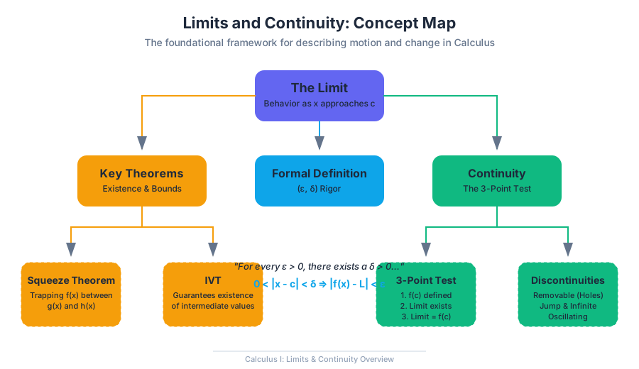
This section explores the formal mechanics of limits, the rigorous definition of continuity, and the foundational theorems—Squeeze and Intermediate Value—that allow us to make certain claims about functions that are otherwise difficult to compute.
The Formal Definition of a Limit
Before we can apply limits to engineering or physics, we must define them with mathematical precision. While the intuitive definition is "the value $L$ that $f(x)$ gets closer to as $x$ gets closer to $c$," this is insufficient for proof-based mathematics.
The formal definition, known as the $(\epsilon, \delta)$-definition of a limit, was popularized by Karl Weierstrass. It removes the "motion" metaphors and replaces them with static inequalities.
Definition: Let $f$ be a function defined on an open interval containing $c$ (except possibly at $c$). We say that: $$\lim_{x \to c} f(x) = L$$ if for every $\epsilon > 0$, there exists a $\delta > 0$ such that if $0 < |x - c| < \delta$, then $|f(x) - L| < \epsilon$.
In plain English: If you pick a tiny distance $\epsilon$ away from the limit $L$, I can find a tiny distance $\delta$ away from $c$ such that every $x$-value in that range maps to a $y$-value within your $\epsilon$-window.
Limit Laws and Algebraic Manipulation
In practice, we rarely use the $(\epsilon, \delta)$ definition for every calculation. Instead, we rely on Limit Laws.
| Law | Formula | Condition |
|---|---|---|
| Sum Law | $\lim (f(x) + g(x)) = \lim f(x) + \lim g(x)$ | Limits must exist |
| Product Law | $\lim (f(x) \cdot g(x)) = \lim f(x) \cdot \lim g(x)$ | Limits must exist |
| Quotient Law | $\lim \frac{f(x)}{g(x)} = \frac{\lim f(x)}{\lim g(x)}$ | $\lim g(x) \neq 0$ |
| Power Law | $\lim [f(x)]^n = [\lim f(x)]^n$ | $n$ is a positive integer |
| Root Law | $\lim \sqrt[n]{f(x)} = \sqrt[n]{\lim f(x)}$ | Valid for $n$ even if $L > 0$ |
The Squeeze Theorem
The Squeeze Theorem (also known as the Sandwich Theorem or the Pinching Theorem) is a technical tool used to find the limit of a function that is "trapped" between two other functions whose limits are known and equal.
The Logic of the Squeeze
Suppose we have three functions such that $g(x) \leq f(x) \leq h(x)$ for all $x$ in an interval around $c$. If the "outer" functions $g(x)$ and $h(x)$ both converge to the same limit $L$ as $x \to c$, then the "inner" function $f(x)$ has no choice but to also converge to $L$.
Theorem: If $g(x) \leq f(x) \leq h(x)$ when $x$ is near $c$ (except possibly at $c$), and $\lim_{x \to c} g(x) = \lim_{x \to c} h(x) = L$, then $\lim_{x \to c} f(x) = L$.
Worked Example: $\lim_{x \to 0} x^2 \sin(\frac{1}{x})$
The function $\sin(\frac{1}{x})$ oscillates infinitely fast as $x$ approaches 0, making the limit difficult to evaluate directly. However, we know the range of the sine function is bounded: $$-1 \leq \sin\left(\frac{1}{x}\right) \leq 1$$ Multiplying the entire inequality by $x^2$ (which is always non-negative): $$-x^2 \leq x^2 \sin\left(\frac{1}{x}\right) \leq x^2$$ As $x \to 0$, both $-x^2 \to 0$ and $x^2 \to 0$. Therefore, by the Squeeze Theorem: $$\lim_{x \to 0} x^2 \sin\left(\frac{1}{x}\right) = 0$$
Continuity: The Three-Point Requirement
In introductory algebra, continuity is often described as "being able to draw the graph without lifting your pencil." In calculus, we require a more rigorous three-part test.
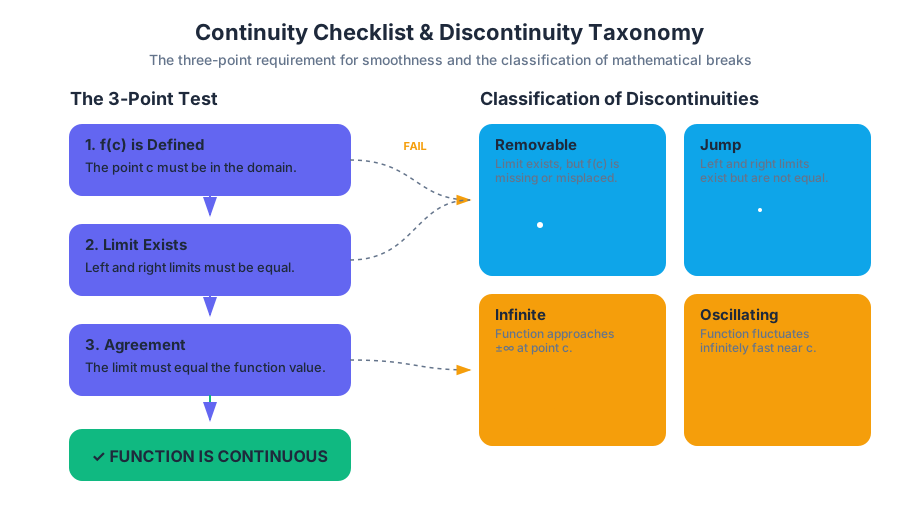
Definition: A function $f(x)$ is continuous at a point $x = c$ if and only if:
- $f(c)$ is defined ($c$ is in the domain).
- $\lim_{x \to c} f(x)$ exists.
- $\lim_{x \to c} f(x) = f(c)$.
If any of these three conditions fail, the function is discontinuous at $c$. Continuity over an interval $[a, b]$ means the function is continuous at every point in $(a, b)$ and possesses one-sided continuity at the endpoints.
Discontinuity Classification
Not all discontinuities are created equal. Engineers and mathematicians categorize them based on how they behave and whether they can be "fixed."
| Type | Description | Graphical Representation | Removable? |
|---|---|---|---|
| Removable | The limit exists, but $f(c)$ is either undefined or different from the limit. | A "hole" in the graph. | Yes (by redefining $f(c)$) |
| Jump | The left-hand limit and right-hand limit both exist but are not equal. | The graph "steps" up or down. | No |
| Infinite | The function approaches $\pm \infty$ as $x$ approaches $c$. | A vertical asymptote. | No |
| Oscillating | The function oscillates infinitely between values as it approaches $c$. | High-frequency "noise" (e.g., $\sin(1/x)$). | No |
The Intermediate Value Theorem (IVT)
The Intermediate Value Theorem is an "existence theorem." It doesn't tell you where a specific value occurs, but it guarantees that the value must exist within a certain interval.
Theorem: If $f$ is continuous on a closed interval $[a, b]$, and $k$ is any number between $f(a)$ and $f(b)$, then there exists at least one number $c$ in $[a, b]$ such that $f(c) = k$.
Practical Application: Root Finding
The IVT is the mathematical basis for the Bisection Method used in computer science to find roots of equations. If a continuous function is negative at $x=a$ and positive at $x=b$, there must be at least one root (where $f(x)=0$) between $a$ and $b$.
Infinite Limits and Asymptotes
When we discuss limits, we often encounter cases where the value of the function grows without bound.
Limits at Infinity ($x \to \infty$)
This describes the end behavior of a function. For rational functions $f(x) = \frac{P(x)}{Q(x)}$, the limit at infinity is determined by the degrees of the polynomials.
- Degree of Numerator < Degree of Denominator: The horizontal asymptote is $y = 0$.
- Degree of Numerator = Degree of Denominator: The horizontal asymptote is the ratio of the leading coefficients.
- Degree of Numerator > Degree of Denominator: There is no horizontal asymptote (the limit is $\pm \infty$).
Infinite Limits ($\lim f(x) = \infty$)
This occurs when the function approaches a vertical asymptote. This usually happens when the denominator of a simplified rational function equals zero.
\text{Example of Vertical Asymptote Behavior:} \\
f(x) = \frac{1}{x-2} \\
\lim_{x \to 2^+} \frac{1}{x-2} = \infty \\
\lim_{x \to 2^-} \frac{1}{x-2} = -\infty
Common Pitfalls and Misconceptions
- Confusing "Approaching" with "Being": A limit describes what happens near $c$. The value of $f(c)$ is irrelevant to the existence of the limit.
- Ignoring One-Sided Limits: A limit exists if and only if the left-hand limit equals the right-hand limit. If $\lim_{x \to c^-} f(x) \neq \lim_{x \to c^+} f(x)$, the limit does not exist (DNE).
- The "Infinity is a Number" Fallacy: When we say $\lim f(x) = \infty$, we are describing a behavior (unbounded growth), not stating that the limit is a specific value. In many contexts, an infinite limit is still considered to "not exist" in the finite sense.
- IVT Requirements: The Intermediate Value Theorem only applies if the function is continuous. Applying IVT to a step function or a function with a vertical asymptote will lead to false conclusions.
Summary of Limit Evaluation Strategies
When faced with a limit problem, follow this hierarchy of strategies:
| Step | Strategy | Action |
|---|---|---|
| 1 | Direct Substitution | Plug in $x=c$. If you get a real number, you're done (if $f$ is continuous). |
| 2 | Factoring/Simplification | If you get $0/0$, look for common factors to cancel (Removable Discontinuity). |
| 3 | Rationalization | If square roots are present, multiply by the conjugate. |
| 4 | Special Trig Limits | Use known limits like $\lim_{x \to 0} \frac{\sin x}{x} = 1$. |
| 5 | Squeeze Theorem | Use if the function is bounded by two simpler functions. |
| 6 | L'Hôpital's Rule | (Advanced) Use derivatives for indeterminate forms like $0/0$ or $\infty/\infty$. |
Source Materials
Study AP/College Calculus BC on Lykke
This course page is free to open: signed out, you can read its first two sections, and signing in, on any plan, opens the rest. The free Lykke Chrome extension syncs your own Canvas courses, so ChatGPT, Claude and Muse can answer from your classes and deadlines. It only reads Canvas.
Add the free extensionSign in to open every sectionAll sections of AP/College Calculus BC · Browse more course pages