From the free course AP/College Calculus BC on Lykke
Integration and Accumulation of Change
Key concepts: Riemann Sums · Fundamental Theorem of Calculus · U-Substitution · Integration by Parts
Introduction to the definite integral, Riemann sums, and the Fundamental Theorem of Calculus.
Integration and Accumulation of Change
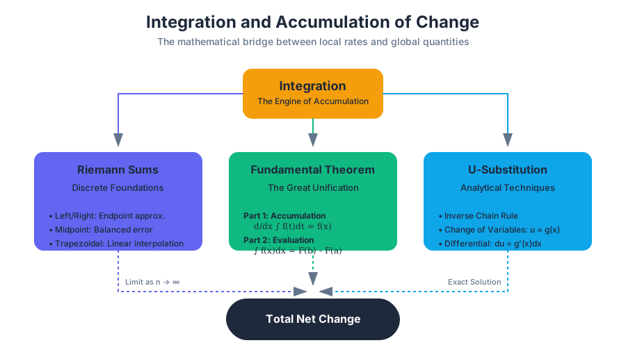
Integration is the mathematical engine of accumulation. While differentiation allows us to zoom in on a single point to find a local rate of change, integration allows us to zoom out, summing those infinitesimal changes to reconstruct the whole. It is the bridge between the local and the global—the process of finding a total quantity when only the rate of its growth is known.
In the context of the AP® Calculus BC curriculum and broader mathematical analysis, this section moves beyond simple "area under a curve" to explore the rigorous foundations of the Definite Integral, the mechanics of the Fundamental Theorem of Calculus, and the sophisticated techniques required to solve complex analytical problems.
Riemann Sums: The Discrete Foundation
Before we can define the integral as a continuous operator, we must understand it as the limit of a discrete sum. A Riemann Sum is an approximation of the area under a curve on a closed interval $[a, b]$ by dividing the area into several geometric shapes (usually rectangles or trapezoids).
The Formal Definition
For a function $f(x)$ defined on $[a, b]$, we partition the interval into $n$ subintervals of width $\Delta x = \frac{b-a}{n}$. The Riemann Sum is defined as:
$$S_n = \sum_{i=1}^{n} f(x_i^*) \Delta x$$
where $x_i^*$ is a sample point in the $i$-th subinterval. As $n \to \infty$, if the function is continuous, this sum converges to the Definite Integral.
Types of Riemann Sums
The choice of the sample point $x_i^*$ determines the type of sum and the nature of the approximation error.
| Method | Sample Point ($x_i^*$) | Characteristic | Error Behavior |
|---|---|---|---|
| Left Riemann Sum | Left endpoint of subinterval | Underestimates increasing functions | $O(\Delta x)$ |
| Right Riemann Sum | Right endpoint of subinterval | Overestimates increasing functions | $O(\Delta x)$ |
| Midpoint Rule | Center of subinterval | Highly accurate; balances error | $O(\Delta x^2)$ |
| Trapezoidal Rule | Average of endpoints | Uses trapezoids instead of rectangles | $O(\Delta x^2)$ |
The Trapezoidal Rule Derivation
The Trapezoidal Rule is often more efficient than endpoint sums because it accounts for the slope of the function. The area of a single trapezoid is $\frac{1}{2}(f(x_{i-1}) + f(x_i))\Delta x$. Summing these across the interval yields the composite Trapezoidal Rule:
$$T_n = \frac{\Delta x}{2} \left[ f(x_0) + 2f(x_1) + 2f(x_2) + \dots + 2f(x_{n-1}) + f(x_n) \right]$$
The Fundamental Theorem of Calculus (FTC)
The Fundamental Theorem of Calculus is the "Great Unification" of mathematics. It establishes that differentiation and integration are inverse processes, effectively linking the geometry of area to the algebra of rates.
FTC Part 1: The Accumulation Function
The first part of the theorem describes the derivative of an accumulation function. If $f$ is continuous on $[a, b]$, then the function $g(x)$ defined by:
$$g(x) = \int_{a}^{x} f(t) , dt$$
is continuous on $[a, b]$, differentiable on $(a, b)$, and its derivative is:
$$g'(x) = f(x)$$
Insight: This tells us that the rate at which area accumulates under $f(t)$ at the point $x$ is exactly the value of the function $f(x)$.
FTC Part 2: Evaluation of Definite Integrals
The second part provides the practical tool for calculating integrals without limits of sums. If $F$ is any antiderivative of $f$ (meaning $F' = f$), then:
$$\int_{a}^{b} f(x) , dx = F(b) - F(a)$$
Comparison of FTC Applications
| Feature | FTC Part 1 (Accumulation) | FTC Part 2 (Evaluation) |
|---|---|---|
| Primary Goal | To find the derivative of an integral | To find the numeric value of an integral |
| Input | A function defined as an integral | A definite integral with fixed bounds |
| Output | A function ($f(x)$) | A scalar value ($C$) |
| Key Use Case | Solving differential equations | Finding area, volume, or net change |
Integration Techniques: U-Substitution
U-Substitution is the integration equivalent of the Chain Rule. It is used to simplify an integral by changing the variable of integration to a new variable $u$, which represents a "nested" function within the integrand.
The Mechanics
If we have an integral of the form $\int f(g(x))g'(x) , dx$, we let $u = g(x)$. Then, the differential $du = g'(x) , dx$. The integral transforms into:
$$\int f(u) , du$$
Worked Example: Definite Integral with U-Sub
Evaluate $\int_{0}^{\sqrt{\pi}} x \sin(x^2) , dx$.
- Identify $u$: Let $u = x^2$.
- Find $du$: $du = 2x , dx \implies \frac{1}{2}du = x , dx$.
- Change Bounds:
- Lower: If $x = 0$, $u = 0^2 = 0$.
- Upper: If $x = \sqrt{\pi}$, $u = (\sqrt{\pi})^2 = \pi$.
- Substitute and Integrate: $$\frac{1}{2} \int_{0}^{\pi} \sin(u) , du = \frac{1}{2} [-\cos(u)]_{0}^{\pi}$$ $$\frac{1}{2} [-\cos(\pi) - (-\cos(0))] = \frac{1}{2} [1 + 1] = 1$$
\begin{aligned}
\text{Step 1: } & u = g(x) \\
\text{Step 2: } & \frac{du}{dx} = g'(x) \implies du = g'(x)dx \\
\text{Step 3: } & \int f(g(x))g'(x)dx = \int f(u)du \\
\text{Step 4: } & \text{Integrate } F(u) + C \\
\text{Step 5: } & \text{Back-substitute } F(g(x)) + C
\end{aligned}
Integration by Parts (IBP)
Where U-substitution reverses the Chain Rule, Integration by Parts reverses the Product Rule. It is the primary tool for integrating the product of two functions, especially when one function simplifies upon differentiation and the other is easily integrable.
The Derivation
Starting with the Product Rule: $$\frac{d}{dx}[uv] = u\frac{dv}{dx} + v\frac{du}{dx}$$ Integrating both sides and rearranging gives the IBP formula:
$$\int u , dv = uv - \int v , du$$
Choosing $u$: The LIATE Rule
The success of IBP depends entirely on the choice of $u$. We use the LIATE mnemonic to prioritize which function should be assigned to $u$:
| Priority | Category | Examples |
|---|---|---|
| L | Logarithmic Functions | $\ln(x), \log_2(x)$ |
| I | Inverse Trigonometric | $\arctan(x), \arcsin(x)$ |
| A | Algebraic Functions | $x^2, 3x, \sqrt{x}$ |
| T | Trigonometric Functions | $\sin(x), \cos(x)$ |
| E | Exponential Functions | $e^x, 2^x$ |
Tabular Integration (The DI Method)
For integrals requiring multiple rounds of IBP (like $\int x^3 e^x , dx$), the "DI Method" is a high-speed alternative to the standard formula. You create two columns: D (to be differentiated) and I (to be integrated).
- List $u$ and its successive derivatives in the D column until you reach 0.
- List $dv$ and its successive integrals in the I column.
- Assign alternating signs (+, -, +, -) to the rows.
- Multiply diagonally.
Real-World Context: Signal Processing
In electrical engineering, integration by parts is used to compute the Fourier Transform, which decomposes signals into their constituent frequencies.
Advanced Accumulation: Improper Integrals
In many physics and statistics applications, we encounter integrals where the interval of integration is infinite or the integrand has a vertical asymptote. These are Improper Integrals.
Type 1: Infinite Intervals
$$\int_{a}^{\infty} f(x) , dx = \lim_{t \to \infty} \int_{a}^{t} f(x) , dx$$ If the limit exists as a finite number, the integral converges. If not, it diverges.
Type 2: Discontinuous Integrands
If $f(x)$ has an infinite discontinuity at $b$: $$\int_{a}^{b} f(x) , dx = \lim_{t \to b^-} \int_{a}^{t} f(x) , dx$$
The p-Series Test for Integrals
A critical shortcut for convergence: $$\int_{1}^{\infty} \frac{1}{x^p} , dx \text{ converges if } p > 1, \text{ and diverges if } p \leq 1.$$
Common Pitfalls and Misconceptions
- Forgetting the Constant of Integration ($+C$): When performing indefinite integration, the result is a family of functions. Omitting $+C$ is a failure to acknowledge the vertical shift.
- Ignoring Discontinuities: Applying FTC Part 2 to a function with a vertical asymptote in the middle of the interval (e.g., $\int_{-1}^{1} \frac{1}{x^2} , dx$) will yield a nonsense result. You must split the integral and use limits.
- Incorrect U-Substitution Bounds: A common error is substituting $u$ but keeping the $x$-limits. Always transform the bounds or back-substitute before evaluating.
- Misidentifying $u$ in IBP: Choosing an exponential for $u$ and a polynomial for $dv$ usually makes the integral more complicated rather than less. Stick to LIATE.
Source Materials
Study AP/College Calculus BC on Lykke
This course page is free to open: signed out, you can read its first two sections, and signing in, on any plan, opens the rest. The free Lykke Chrome extension syncs your own Canvas courses, so ChatGPT, Claude and Muse can answer from your classes and deadlines. It only reads Canvas.
Add the free extensionSign in to open every sectionAll sections of AP/College Calculus BC · Browse more course pages