From the free course AP/College Calculus BC on Lykke
Differential Equations
Key concepts: Slope Fields · Euler's Method · Separation of Variables · Logistic Growth
Solving and modeling equations that involve derivatives.
Differential Equations
Differential equations (DEs) represent the pinnacle of the calculus sequence, serving as the bridge between abstract mathematical theory and the physical reality of a changing world. While standard calculus focuses on finding the rate of change of a known function, differential equations invert this relationship: we are given the rate of change (the derivative) and must reconstruct the original function.
In the words of the physicist Richard Feynman, "The laws of nature are expressed as differential equations." From the cooling of a cup of coffee to the vibrations of a bridge or the spread of a viral pathogen, differential equations provide the rigorous framework necessary to model, predict, and control dynamic systems.
The Fundamental Landscape of Differential Equations
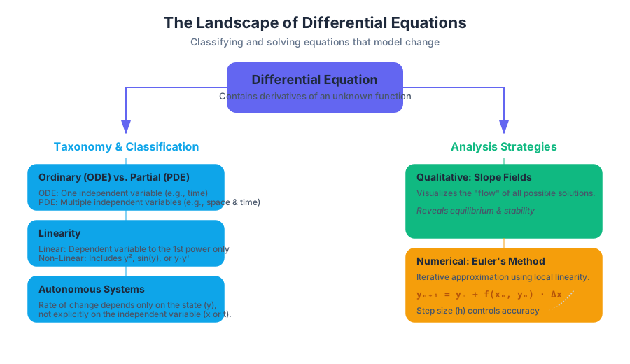
A differential equation is any equation that contains one or more derivatives of an unknown function. The order of the equation is determined by the highest derivative present. In introductory contexts, we focus primarily on First-Order Ordinary Differential Equations (ODEs), which take the general form:
$$\frac{dy}{dx} = f(x, y)$$
Where $y$ is an unknown function of $x$. Solving such an equation means finding a function $y = \phi(x)$ that satisfies the relationship for all $x$ in a given interval.
Classification and Terminology
To navigate this field, one must understand the taxonomy of DEs:
| Term | Definition | Example |
|---|---|---|
| Ordinary (ODE) | Contains derivatives with respect to only one independent variable. | $\frac{dy}{dx} + 5y = e^x$ |
| Partial (PDE) | Contains derivatives with respect to multiple independent variables. | $\frac{\partial^2 u}{\partial t^2} = c^2 \frac{\partial^2 u}{\partial x^2}$ |
| Linear | The dependent variable and its derivatives appear only to the first power. | $y'' + 3y' + 2y = 0$ |
| Non-Linear | The dependent variable or its derivatives are multiplied together or involve non-linear functions. | $\frac{dy}{dx} = y^2 + \sin(y)$ |
| Autonomous | The rate of change depends only on the dependent variable, not the independent one. | $\frac{dy}{dt} = ky(1 - \frac{y}{K})$ |
Slope Fields: Visualizing the Derivative
When an analytical solution to a differential equation is difficult or impossible to find, we turn to qualitative analysis. Slope Fields (or direction fields) are the primary tool for this.
What it is
A slope field is a graphical representation of the slopes of all possible solution curves for a first-order DE. At every point $(x, y)$ in the plane, we draw a small line segment with a slope equal to $f(x, y)$.
Why it matters
Slope fields allow us to visualize the "flow" of a system. Even without solving the equation, we can determine the long-term behavior (asymptotic behavior) of a solution and identify equilibrium points where $dy/dx = 0$.
Construction and Interpretation
To construct a slope field for $\frac{dy}{dx} = x - y$:
- Select a grid of points (e.g., integers from -3 to 3).
- Calculate the value of $x - y$ at each point.
- Draw a short segment with that calculated slope at that point.
Theorem: Existence and Uniqueness If $f(x, y)$ and $\frac{\partial f}{\partial y}$ are continuous in a region containing $(x_0, y_0)$, then there exists a unique solution curve passing through that point. This ensures that solution curves in a slope field never cross.
Euler's Method: Numerical Approximation
Not every differential equation can be solved with pen and paper. In engineering and computational science, we often use Euler's Method, the most fundamental numerical technique for approximating the solution to an Initial Value Problem (IVP).
Mechanics of the Algorithm
Euler's Method relies on the concept of local linearity. If we know a starting point $(x_0, y_0)$ and the slope at that point $f(x_0, y_0)$, we can move a small distance $\Delta x$ (the step size) along the tangent line to find an approximate next point $(x_1, y_1)$.
The iterative formulas are:
- $x_{n+1} = x_n + \Delta x$
- $y_{n+1} = y_n + f(x_n, y_n) \cdot \Delta x$
Worked Example
Approximate $y(1.2)$ for $\frac{dy}{dx} = x + y$ with initial condition $y(1) = 0$ and step size $\Delta x = 0.1$.
- Step 1: $x_0 = 1, y_0 = 0$. Slope $m = 1+0 = 1$. $y_1 = 0 + (1)(0.1) = 0.1$. New point: $(1.1, 0.1)$.
- Step 2: $x_1 = 1.1, y_1 = 0.1$. Slope $m = 1.1 + 0.1 = 1.2$. $y_2 = 0.1 + (1.2)(0.1) = 0.22$. New point: $(1.2, 0.22)$.
The approximation for $y(1.2)$ is $0.22$.
Error Analysis
Euler's method is a first-order method, meaning the local truncation error is $O(h^2)$ and the global truncation error is $O(h)$.
| Factor | Effect on Accuracy | Trade-off |
|---|---|---|
| Step Size ($h$) | Smaller $h$ reduces truncation error. | Increases computational cost and round-off error. |
| Curvature ($y''$) | High curvature increases error (linear approximation fails). | Requires adaptive step-size methods (like Runge-Kutta). |
| Interval Length | Errors accumulate over longer intervals. | May require more sophisticated "multi-step" methods. |
Separation of Variables: Analytical Precision
Separation of Variables is the primary algebraic technique for solving first-order DEs. It is applicable when the derivative can be factored into a product of a function of $x$ and a function of $y$.
The Derivation
Given $\frac{dy}{dx} = g(x)h(y)$, we assume $h(y) \neq 0$ and rewrite the equation:
\begin{aligned}
\frac{1}{h(y)} dy &= g(x) dx \\
\int \frac{1}{h(y)} dy &= \int g(x) dx \\
H(y) &= G(x) + C
\end{aligned}
This yields an implicit solution. If possible, we solve for $y$ to get the explicit solution.
Worked Example: The Particular Solution
Solve $\frac{dy}{dx} = \frac{2x}{y}$ with the initial condition $y(0) = -3$.
- Separate: $y , dy = 2x , dx$
- Integrate: $\int y , dy = \int 2x , dx \implies \frac{1}{2}y^2 = x^2 + C$
- Apply Initial Condition: $\frac{1}{2}(-3)^2 = (0)^2 + C \implies C = 4.5$
- Solve for y: $\frac{1}{2}y^2 = x^2 + 4.5 \implies y^2 = 2x^2 + 9 \implies y = \pm\sqrt{2x^2 + 9}$
- Select Branch: Since $y(0) = -3$, we must choose the negative root: $y = -\sqrt{2x^2 + 9}$.
Common Pitfalls
- The Constant of Integration ($C$): Forgetting $C$ is the most common error. $C$ must be introduced the moment the integral is performed, not added at the end.
- Absolute Values: When integrating $1/y$, the result is $\ln|y|$. Removing the natural log requires $e^{\ln|y|} = e^{f(x)+C}$, which becomes $|y| = e^C e^{f(x)}$. This is often simplified to $y = Ae^{f(x)}$, where $A = \pm e^C$.
- Singular Solutions: Dividing by $h(y)$ assumes $h(y) \neq 0$. Values of $y$ that make $h(y) = 0$ are constant solutions that might be missed by the separation process.
Growth Models: Exponential vs. Logistic
Differential equations are the standard for modeling population dynamics. We generally distinguish between "unconstrained" and "constrained" growth.
Exponential Growth
The simplest model assumes the rate of growth is proportional to the current population: $$\frac{dP}{dt} = kP$$ Using separation of variables, this yields the familiar $P(t) = P_0 e^{kt}$. While accurate for short periods, it fails for long-term modeling because it ignores resource limits.
Logistic Growth
The Logistic Model introduces a Carrying Capacity ($K$), the maximum population the environment can sustain. The rate of growth is proportional to both the current population and the remaining "room" for growth.
$$\frac{dP}{dt} = kP \left( 1 - \frac{P}{K} \right)$$
Solving the Logistic Equation
This equation is solved using separation of variables and partial fraction decomposition:
\begin{aligned}
\int \frac{dP}{P(1 - P/K)} &= \int k \, dt \\
\int \left( \frac{1}{P} + \frac{1/K}{1 - P/K} \right) dP &= kt + C \\
\ln|P| - \ln|1 - P/K| &= kt + C \\
\ln \left| \frac{P}{1 - P/K} \right| &= kt + C
\end{aligned}
Solving for $P$ gives the general solution: $$P(t) = \frac{K}{1 + Ae^{-kt}}$$ where $A = \frac{K - P_0}{P_0}$.
Key Features of Logistic Growth
| Feature | Mathematical Condition | Physical Meaning |
|---|---|---|
| Max Growth Rate | $P = K/2$ | The population grows fastest when it is half-full. |
| Inflection Point | $\frac{d^2P}{dt^2} = 0$ | The point where growth shifts from accelerating to decelerating. |
| Asymptote | $\lim_{t \to \infty} P(t) = K$ | The population stabilizes at the carrying capacity. |
| Equilibrium | $P=0$ or $P=K$ | Points where the population does not change. |
Advanced Tooling: Symbolic Computation
In professional practice, we often use symbolic engines to verify solutions or handle complex integration.
Summary of Methods
| Method | Best Used When... | Pros | Cons |
|---|---|---|---|
| Slope Fields | Qualitative behavior is needed. | No integration required; handles non-linearities. | No exact numerical values. |
| Euler's Method | No analytical solution exists. | Easy to program; works on almost any DE. | Accumulates error; requires small steps. |
| Separation of Variables | Equation is of the form $f(y)dy = g(x)dx$. | Provides exact, analytical functions. | Only works for a small subset of DEs. |
| Growth Models | Modeling biological or social systems. | Highly predictive for real-world data. | Requires estimating parameters like $k$ and $K$. |
Source Materials
Study AP/College Calculus BC on Lykke
This course page is free to open: signed out, you can read its first two sections, and signing in, on any plan, opens the rest. The free Lykke Chrome extension syncs your own Canvas courses, so ChatGPT, Claude and Muse can answer from your classes and deadlines. It only reads Canvas.
Add the free extensionSign in to open every sectionAll sections of AP/College Calculus BC · Browse more course pages