From the free course AP/College Calculus BC on Lykke
Contextual Applications of Differentiation
Key concepts: Straight-line Motion · Related Rates · Local Linearity · L'Hôpital's Rule
Applying derivatives to real-world scenarios like motion and related rates.
Contextual Applications of Differentiation
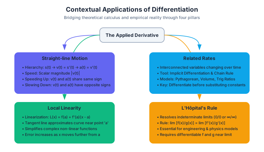
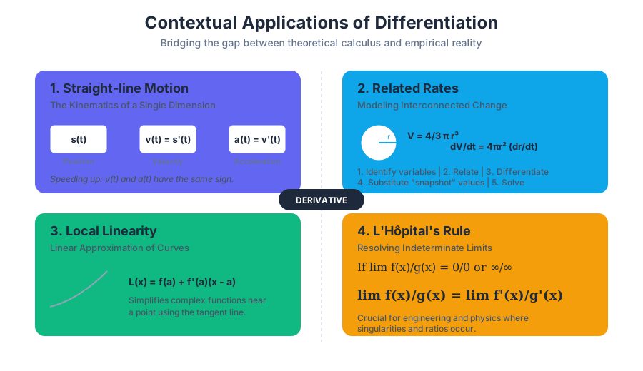
In the abstract realm of calculus, the derivative is defined as the limit of a difference quotient—a purely mathematical construct representing the slope of a tangent line. However, the true power of the derivative is realized when we step out of the Cartesian plane and into the physical world. Contextual Applications of Differentiation bridge the gap between theoretical calculus and empirical reality, providing the mathematical framework to describe motion, optimize systems, and approximate complex behaviors.
This section explores four pillars of applied differentiation: Straight-line Motion, where we track the kinematics of particles; Related Rates, where we model interconnected variables changing over time; Local Linearity, which allows us to simplify complex curves into manageable lines; and L'Hôpital's Rule, a rigorous tool for resolving indeterminate limits encountered in engineering and physics.
Straight-line Motion: The Kinematics of a Single Dimension
Straight-line motion (or rectilinear motion) is the study of an object moving along a fixed path, typically represented by a coordinate axis. In this context, the derivative is not just a slope; it is a physical rate of change.
The Hierarchy of Motion
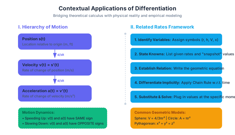
We define the state of a particle using three primary functions of time $t$:
- Position $s(t)$: The location of the particle relative to an origin.
- Velocity $v(t) = s'(t)$: The rate of change of position. It indicates both speed and direction.
- Acceleration $a(t) = v'(t) = s''(t)$: The rate of change of velocity.
Definition: Speed vs. Velocity While velocity $v(t)$ is a vector quantity (it can be negative, indicating motion in the "left" or "down" direction), speed is a scalar quantity defined as the absolute value of velocity: $|v(t)|$.
Interpreting Motion Dynamics
To fully understand a particle's behavior, we must analyze the signs of these derivatives.
| Condition | Physical Interpretation |
|---|---|
| $v(t) > 0$ | Particle is moving in the positive direction (Right/Up). |
| $v(t) < 0$ | Particle is moving in the negative direction (Left/Down). |
| $v(t) = 0$ | Particle is momentarily at rest (potential turnaround point). |
| $v(t)$ and $a(t)$ have the same sign | The particle is speeding up. |
| $v(t)$ and $a(t)$ have opposite signs | The particle is slowing down (decelerating). |
Worked Example: Analyzing a Moving Particle
Consider a particle moving along the $x$-axis with position function $s(t) = t^3 - 6t^2 + 9t$ for $t \ge 0$.
- Find Velocity: $v(t) = 3t^2 - 12t + 9 = 3(t-1)(t-3)$.
- Find Acceleration: $a(t) = 6t - 12 = 6(t-2)$.
- Determine Rest Points: The particle is at rest when $v(t) = 0$, which occurs at $t=1$ and $t=3$.
- Intervals of Motion:
- $0 \le t < 1$: $v(t) > 0$ (Moving Right)
- $1 < t < 3$: $v(t) < 0$ (Moving Left)
- $t > 3$: $v(t) > 0$ (Moving Right)
Related Rates: Modeling Interconnected Change
In many real-world systems, several variables change simultaneously, and their rates of change are linked by a geometric or physical constraint. Related Rates problems use the Chain Rule to find one rate of change in terms of others.
The Procedural Framework
Solving a related rates problem requires a disciplined approach to avoid "premature substitution"—the most common error where students plug in constant values before differentiating.
- Identify Variables: Assign symbols to all changing quantities (e.g., $r$ for radius, $h$ for height, $V$ for volume).
- State the Knowns: Write down the given rates (e.g., $dr/dt = 2$) and the specific "snapshot" moment (e.g., when $r=5$).
- Establish the Relation: Write an equation relating the variables (e.g., $V = \frac{1}{3}\pi r^2 h$).
- Differentiate Implicitly: Differentiate both sides with respect to time $t$.
- Substitute and Solve: Plug in the known values at the specific moment and solve for the unknown rate.
Common Geometric Models
| Shape / Scenario | Primary Equation | Differentiated Form (Example) |
|---|---|---|
| Sphere (Volume) | $V = \frac{4}{3}\pi r^3$ | $\frac{dV}{dt} = 4\pi r^2 \frac{dr}{dt}$ |
| Right Triangle (Pythagorean) | $x^2 + y^2 = z^2$ | $2x\frac{dx}{dt} + 2y\frac{dy}{dt} = 2z\frac{dz}{dt}$ |
| Conical Tank (Volume) | $V = \frac{1}{3}\pi r^2 h$ | Requires substitution of $r$ in terms of $h$ first. |
| Circle (Area) | $A = \pi r^2$ | $\frac{dA}{dt} = 2\pi r \frac{dr}{dt}$ |
Worked Example: The Sliding Ladder
A 10-foot ladder leans against a wall. The bottom of the ladder is pulled away from the wall at a rate of 2 ft/s. How fast is the top of the ladder sliding down the wall when the bottom is 6 feet from the wall?
% Mathematical Derivation for the Sliding Ladder
% Let x = distance from wall to base, y = height of ladder top.
% Constraint: x^2 + y^2 = 10^2 (Pythagorean Theorem)

1. Given: dx/dt = 2, x = 6.
2. Find: dy/dt when x = 6.
3. Find y when x = 6:
   6^2 + y^2 = 100 => 36 + y^2 = 100 => y = 8.
4. Differentiate constraint w.r.t. t:
   d/dt [x^2 + y^2] = d/dt [100]
   2x(dx/dt) + 2y(dy/dt) = 0
5. Substitute:
   2(6)(2) + 2(8)(dy/dt) = 0
   24 + 16(dy/dt) = 0
   dy/dt = -24/16 = -1.5 ft/s.
% The top is sliding down at 1.5 ft/s.
Local Linearity and Linear Approximation
The principle of Local Linearity suggests that if we zoom in far enough on a differentiable curve, the curve looks like a straight line. This "line" is the tangent line at that point. We use this tangent line to approximate the value of the function near the point of tangency.
The Linearization Formula
The linearization $L(x)$ of a function $f$ at a point $a$ is simply the equation of the tangent line:
$$L(x) = f(a) + f'(a)(x - a)$$
Where:
- $f(a)$ is the "starting" value.
- $f'(a)$ is the slope (rate of change).
- $(x - a)$ is the distance from the known point.
Error and Concavity
The accuracy of a linear approximation depends on the concavity of the original function:
- If $f''(x) > 0$ (Concave Up), the tangent line lies below the curve, resulting in an underestimate.
- If $f''(x) < 0$ (Concave Down), the tangent line lies above the curve, resulting in an overestimate.
Practical Usage: Estimating Roots
To estimate $\sqrt{26}$ without a calculator, we use the function $f(x) = \sqrt{x}$ and the known point $a = 25$.
- $f(25) = \sqrt{25} = 5$.
- $f'(x) = \frac{1}{2\sqrt{x}} \implies f'(25) = \frac{1}{10} = 0.1$.
- $L(x) = 5 + 0.1(x - 25)$.
- $L(26) = 5 + 0.1(26 - 25) = 5.1$.
The actual value of $\sqrt{26} \approx 5.099$. Our approximation is remarkably close.
L'Hôpital's Rule: Resolving Indeterminacy
In the study of limits, we often encounter forms like $0/0$ or $\infty/\infty$. These are indeterminate forms—they do not have a defined value and could represent any real number or even infinity. L'Hôpital's Rule provides a method to evaluate these limits using derivatives.
The Theorem
If $\lim_{x \to c} f(x) = 0$ and $\lim_{x \to c} g(x) = 0$ (or both are $\pm \infty$), and if $g'(x) \neq 0$ near $c$, then: $$\lim_{x \to c} \frac{f(x)}{g(x)} = \lim_{x \to c} \frac{f'(x)}{g'(x)}$$ provided the limit on the right exists or is $\pm \infty$.
Indeterminate vs. Determinate Forms
It is crucial to distinguish between forms that require L'Hôpital's Rule and those that are already solved.
| Form | Status | Action |
|---|---|---|
| $0/0$ | Indeterminate | Apply L'Hôpital |
| $\infty/\infty$ | Indeterminate | Apply L'Hôpital |
| $0 \cdot \infty$ | Indeterminate | Rewrite as $(f) / (1/g)$ then apply |
| $\infty - \infty$ | Indeterminate | Find common denominator / Rationalize |
| $0/ \infty$ | Determinate | Result is $0$ |
| $\infty / 0$ | Determinate | Result is $\pm \infty$ (Undefined) |
| $1^\infty, 0^0, \infty^0$ | Indeterminate | Use natural logs ($\ln$) to convert to $0 \cdot \infty$ |
Pitfalls and Misconceptions
- The Quotient Rule Trap: L'Hôpital's Rule is not the quotient rule. You differentiate the numerator and denominator separately.
- Premature Application: Do not apply the rule if the limit is not indeterminate. For example, $\lim_{x \to 0} \frac{x+5}{x+1} = 5$. Applying L'Hôpital would incorrectly give $\lim_{x \to 0} \frac{1}{1} = 1$.
- Infinite Loops: Sometimes applying the rule repeatedly leads back to the original form (common with $e^x$ and trig functions). In these cases, algebraic manipulation or the Squeeze Theorem may be required.
Worked Example: Transcendental Limits
Evaluate $\lim_{x \to 0} \frac{e^x - 1 - x}{x^2}$.
- Check Form: $\frac{e^0 - 1 - 0}{0^2} = \frac{0}{0}$. (Indeterminate)
- First Application: Differentiate top and bottom. $$\lim_{x \to 0} \frac{e^x - 1}{2x}$$
- Check Form Again: $\frac{e^0 - 1}{2(0)} = \frac{0}{0}$. (Still Indeterminate)
- Second Application: Differentiate again. $$\lim_{x \to 0} \frac{e^x}{2} = \frac{e^0}{2} = \frac{1}{2}$$
Summary of Contextual Applications
The transition from "calculating a derivative" to "applying a derivative" represents the shift from being a student of mathematics to being a practitioner of science. Whether we are predicting the point where a particle reverses direction, calculating the rate at which a reservoir empties, or using a tangent line to estimate a complex square root, we are utilizing the derivative as a tool for understanding change.
The concepts of Straight-line Motion and Related Rates emphasize the derivative as a temporal rate ($d/dt$), while Local Linearity and L'Hôpital's Rule leverage the derivative's ability to describe the local geometry of functions. Together, these tools form the backbone of differential modeling in the modern world.
Source Materials
Study AP/College Calculus BC on Lykke
This course page is free to open: signed out, you can read its first two sections, and signing in, on any plan, opens the rest. The free Lykke Chrome extension syncs your own Canvas courses, so ChatGPT, Claude and Muse can answer from your classes and deadlines. It only reads Canvas.
Add the free extensionSign in to open every sectionAll sections of AP/College Calculus BC · Browse more course pages