From the free course AP/College Calculus BC on Lykke
Applications of Integration
Key concepts: Average Value · Net Change · Area Between Curves · Volume by Cross Sections
Using integrals to find average values, areas between curves, and volumes.
Applications of Integration: From Accumulation to Geometry
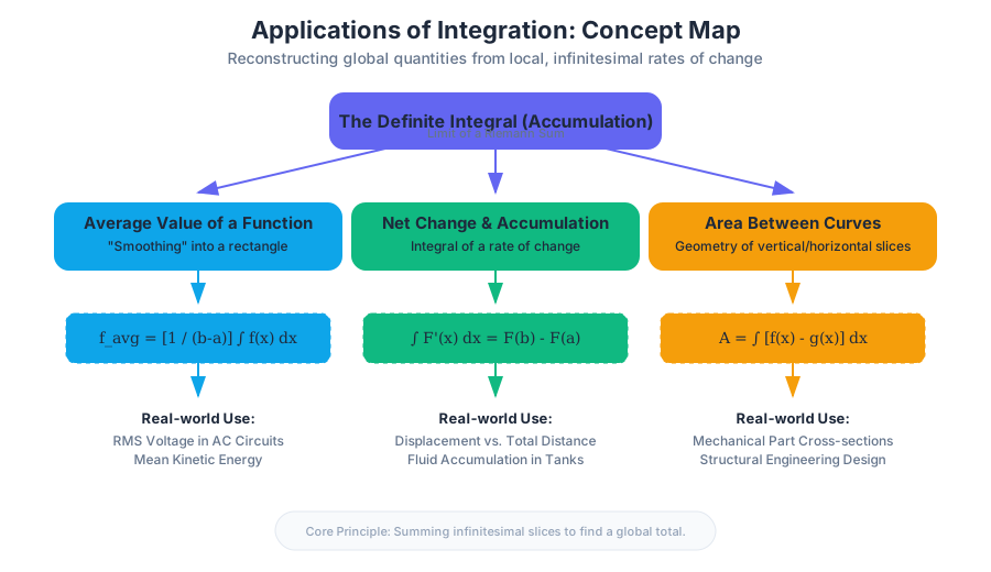
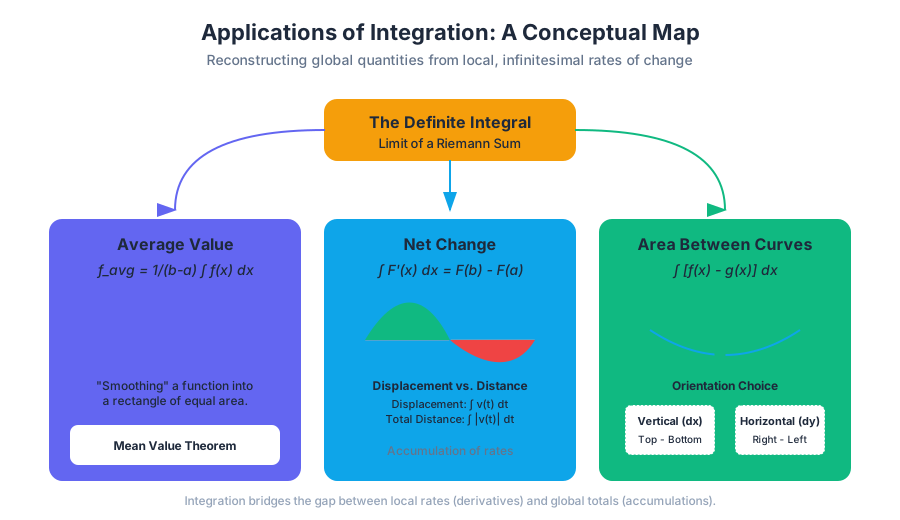
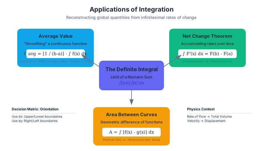
The definite integral is often introduced as the "area under a curve," but this geometric interpretation is merely the surface of a much deeper mathematical well. In the context of advanced calculus and engineering, integration is the fundamental tool for accumulation. It allows us to reconstruct global quantities from local, infinitesimal rates of change. Whether we are determining the average temperature of a cooling engine, the total displacement of a particle under varying acceleration, or the precise volume of a complex mechanical part, we rely on the same underlying principle: the limit of a Riemann sum.
Average Value of a Function
In discrete mathematics, the average of a set of numbers is the sum divided by the count. However, for a continuous function $f(x)$ on an interval $[a, b]$, there are infinitely many points. We cannot sum them individually. Instead, we use the integral to "smooth out" the function into a rectangle with the same area.
1. Definition and Mathematical Notation
The Average Value of a continuous function $f$ over the interval $[a, b]$ is defined as:
Definition: $f_{avg} = \frac{1}{b-a} \int_{a}^{b} f(x) , dx$
This concept is inextricably linked to the Mean Value Theorem for Integrals, which guarantees that for a continuous function, there exists at least one point $c$ in $[a, b]$ such that $f(c) = f_{avg}$.
2. Why It Matters
In thermodynamics, we use average values to find the mean kinetic energy of particles. In electrical engineering, the Root Mean Square (RMS) voltage—a variation of the average value—is used to define the effective voltage of an alternating current (AC).
3. Comparison: Discrete vs. Continuous Average
| Feature | Discrete Average (Arithmetic Mean) | Continuous Average (Integral Mean) |
|---|---|---|
| Input Type | Finite set of points ${x_1, x_2, ... x_n}$ | Continuous function $f(x)$ on $[a, b]$ |
| Summation Method | $\sum_{i=1}^{n} x_i$ | $\int_{a}^{b} f(x) , dx$ |
| Normalization | Divide by $n$ (count) | Divide by $b-a$ (interval length) |
| Physical Analogy | Average height of students in a class | Average height of a mountain range |
Net Change and Accumulation
The Net Change Theorem is a direct application of the Fundamental Theorem of Calculus. It states that the integral of a rate of change is the net change in the original quantity.
1. The Mechanics of Accumulation
If $F'(x)$ represents the rate at which a quantity is changing, then: $$\int_{a}^{b} F'(x) , dx = F(b) - F(a)$$
This is vital in physics when distinguishing between displacement and total distance traveled.
- Displacement: $\int_{t_1}^{t_2} v(t) , dt$ (The net change in position).
- Total Distance: $\int_{t_1}^{t_2} |v(t)| , dt$ (The accumulation of all movement, regardless of direction).
2. Derivation of the Accumulation Function
We can define an accumulation function $S(x)$ that represents the quantity gathered from a starting point $a$ to a variable point $x$:
S(x) = \int_{a}^{x} f(t) \, dt
Where:
- $f(t)$ is the rate of change (e.g., liters per second).
- $S(x)$ is the total amount accumulated (e.g., total liters).
3. Common Pitfalls: Signs and Direction
A common error is neglecting the sign of the function. In a net change problem involving a tank being filled and drained simultaneously, the rate function $R(t) = Inflow(t) - Outflow(t)$ can be negative. The integral will correctly reflect the "net" volume, but if you are asked for the "total volume processed," you must integrate the absolute value.
Area Between Curves
Calculating the area between two curves $f(x)$ and $g(x)$ is the process of integrating the vertical (or horizontal) distance between them over a specific interval.
1. Vertical Slices ($dx$) vs. Horizontal Slices ($dy$)
The choice of orientation depends on the geometry of the functions.
Theorem: If $f(x) \geq g(x)$ for all $x$ in $[a, b]$, the area $A$ is: $A = \int_{a}^{b} [f(x) - g(x)] , dx$
If the functions are defined as $x = f(y)$ and $x = g(y)$, we integrate with respect to $y$: $A = \int_{c}^{d} [right_function(y) - left_function(y)] , dy$
2. Decision Matrix for Integration Orientation
| Scenario | Use $dx$ (Vertical Slices) | Use $dy$ (Horizontal Slices) |
|---|---|---|
| Function Form | $y = f(x)$ | $x = g(y)$ |
| Boundaries | Upper and Lower boundaries are clear | Right and Left boundaries are clear |
| Complexity | Easier if functions pass the Vertical Line Test | Easier if functions pass the Horizontal Line Test |
| Intersection | Find $x$-coordinates of intersection | Find $y$-coordinates of intersection |
3. Worked Example: Finding Intersection Points
To find the area between $y = x^2$ and $y = 2x - x^2$, we must first determine the limits of integration by setting the equations equal: $x^2 = 2x - x^2 \implies 2x^2 - 2x = 0 \implies 2x(x - 1) = 0$. The limits are $x=0$ and $x=1$.
Volume by Cross Sections
This is the most generalized method for finding the volume of a 3D solid. If we know the area of a "slice" of the solid as a function of its position, we can sum those slices to find the total volume.
1. The Slicing Formula
For a solid extending from $x=a$ to $x=b$, where the cross-sectional area perpendicular to the $x$-axis is $A(x)$:
Volume Formula: $V = \int_{a}^{b} A(x) , dx$
2. Common Cross-Sectional Geometries
The difficulty usually lies in expressing $A(x)$ in terms of the side length $s$, which is typically the distance between two curves $f(x)$ and $g(x)$.
| Shape of Cross Section | Area Formula $A(x)$ |
|---|---|
| Square | $s^2$ |
| Semicircle | $\frac{1}{2} \pi (\frac{s}{2})^2 = \frac{\pi s^2}{8}$ |
| Equilateral Triangle | $\frac{\sqrt{3}}{4} s^2$ |
| Isosceles Right Triangle (Leg on base) | $\frac{1}{2} s^2$ |
| Isosceles Right Triangle (Hypotenuse on base) | $\frac{1}{4} s^2$ |
Solids of Revolution: Disk and Washer Methods
A "Solid of Revolution" is a special case of the cross-section method where the cross-sections are always circles or annuli (washers). These are generated by rotating a 2D region around an axis.
1. The Disk Method
Used when the region being rotated is flush against the axis of revolution. The cross-section is a solid disk with radius $R(x)$. $$V = \pi \int_{a}^{b} [R(x)]^2 , dx$$
2. The Washer Method
Used when there is a "gap" between the region and the axis of revolution. The cross-section is a washer (a disk with a hole). $$V = \pi \int_{a}^{b} ([R_{outer}(x)]^2 - [R_{inner}(x)]^2) , dx$$
Crucial Insight: Always identify the radius as the distance from the Axis of Revolution to the function. If rotating around $y=k$, the radius is $|f(x) - k|$.
3. Comparison of Methods
| Method | Cross-Section Shape | Integral Formula | Best For... |
|---|---|---|---|
| Disk | Solid Circle | $\pi \int R^2$ | Single curve against the axis |
| Washer | Ring / Annulus | $\pi \int (R^2 - r^2)$ | Area between two curves |
| Shell | Cylindrical Wall | $2\pi \int r \cdot h$ | Rotation around axis parallel to $y$ (when using $dx$) |
Advanced Application: Arc Length
Integration can also be used to find the length of a smooth curve $y = f(x)$ from $x=a$ to $x=b$. This is derived using the Pythagorean theorem on infinitesimal segments $ds$.
1. Derivation
$ds^2 = dx^2 + dy^2$ $ds = \sqrt{1 + (\frac{dy}{dx})^2} , dx$
Summing these segments gives the Arc Length Formula: $$L = \int_{a}^{b} \sqrt{1 + [f'(x)]^2} , dx$$
Common Pitfalls and Expert Tips
- The "Square the Difference" Trap: In the Washer Method, students often write $\pi \int (R - r)^2 , dx$. This is incorrect. The correct form is the difference of the squares: $\pi \int (R^2 - r^2) , dx$. Geometry dictates that we subtract the area of the inner circle from the area of the outer circle.
- Axis of Rotation: If you rotate around a line other than the x or y axis (e.g., $x = -2$), your radius calculation must account for that shift. The radius is $x - (-2) = x + 2$.
- Variable of Integration: If the boundaries are given in terms of $y$, or the shapes are stacked horizontally, you must convert your functions to $x = f(y)$ and integrate $dy$. Mixing $dx$ limits with $dy$ functions is a frequent source of error in multi-step problems.
- Absolute Value in Net Change: When calculating total distance, finding the roots of the velocity function $v(t) = 0$ is a mandatory first step to split the integral where the particle changes direction.
Source Materials
Study AP/College Calculus BC on Lykke
This course page is free to open: signed out, you can read its first two sections, and signing in, on any plan, opens the rest. The free Lykke Chrome extension syncs your own Canvas courses, so ChatGPT, Claude and Muse can answer from your classes and deadlines. It only reads Canvas.
Add the free extensionSign in to open every sectionAll sections of AP/College Calculus BC · Browse more course pages