From the free course AP/College Calculus BC on Lykke
Analytical Applications of Differentiation
Key concepts: Mean Value Theorem · Extreme Value Theorem · First/Second Derivative Tests · Optimization
Using derivatives to analyze function behavior, including extrema and concavity.
Analytical Applications of Differentiation
In the preceding study of calculus, the focus was primarily on the mechanics of the derivative: the "how" of differentiation. We mastered the Power Rule, the Chain Rule, and the nuances of transcendental functions. However, the true power of calculus lies in its analytical applications. By examining the derivative of a function, we gain a profound understanding of the function’s geometry, its limits, and its optimal states.
This section serves as the bridge between pure calculation and applied mathematics. We will explore how derivatives allow us to reconstruct the "story" of a function—identifying where it peaks, where it plunges, and how it bends. These tools are the foundation of modern engineering, economic modeling, and physical simulations.
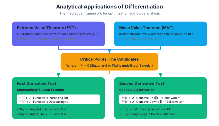
The Extreme Value Theorem (EVT) and Critical Points
Before we can optimize a system, we must guarantee that an optimum actually exists. The Extreme Value Theorem (EVT) provides this theoretical bedrock.
What it is
The EVT states that if a function $f$ is continuous on a closed interval $[a, b]$, then $f$ must attain both an absolute maximum and an absolute minimum on that interval.
The Extreme Value Theorem: Let $f$ be continuous on the closed interval $[a, b]$. There exist numbers $c$ and $d$ in $[a, b]$ such that $f(c) \leq f(x) \leq f(d)$ for all $x$ in $[a, b]$.
Why it matters
In real-world constraints (e.g., a finite budget, a specific range of temperatures, a fixed amount of material), we need to know that a "best" and "worst" case exist. Without the requirement of a closed interval and continuity, a function could head toward infinity or approach a value it never actually reaches, leaving the optimization problem unsolvable.
How it works: The Candidates Test
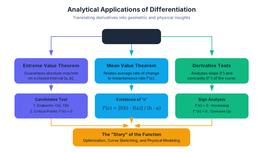
To find these absolute extrema, we use the Candidates Test. We look at two types of points:
- Critical Points: Values of $x$ where $f'(x) = 0$ or $f'(x)$ is undefined.
- Endpoints: The boundaries $a$ and $b$ of the interval.
| Point Type | Condition | Significance |
|---|---|---|
| Stationary Point | $f'(x) = 0$ | The tangent line is horizontal; potential peak or valley. |
| Singular Point | $f'(x)$ is undefined | A cusp, corner, or vertical tangent; potential extremum. |
| Boundary Point | $x = a$ or $x = b$ | The limits of the domain; often where the absolute max/min resides. |
The Mean Value Theorem (MVT)
If the EVT guarantees the existence of a destination, the Mean Value Theorem (MVT) describes the relationship between the journey and the average speed.
What it is
The MVT states that for a sufficiently smooth curve, there is at least one point where the instantaneous rate of change (the derivative) equals the average rate of change over an interval.
Mean Value Theorem: If $f$ is continuous on $[a, b]$ and differentiable on $(a, b)$, then there exists at least one point $c$ in $(a, b)$ such that: $$f'(c) = \frac{f(b) - f(a)}{b - a}$$
Mathematical Derivation
The MVT is a generalization of Rolle's Theorem, which covers the specific case where $f(a) = f(b)$.
1. Define a helper function g(x) that represents the vertical distance
   between f(x) and the secant line connecting (a, f(a)) and (b, f(b)).

   g(x) = f(x) - [f(a) + ((f(b) - f(a))/(b - a)) * (x - a)]

2. Note that g(a) = 0 and g(b) = 0.
3. Since f is continuous and differentiable, g is also continuous and differentiable.
4. By Rolle's Theorem, there must be some c in (a, b) such that g'(c) = 0.
5. Differentiate g(x):
   g'(x) = f'(x) - (f(b) - f(a))/(b - a)
6. Set g'(c) = 0:
   0 = f'(c) - (f(b) - f(a))/(b - a)
   f'(c) = (f(b) - f(a))/(b - a)
Concrete Example: Speed Traps
Imagine a car enters a toll road at 12:00 PM and exits 100 miles later at 1:20 PM (1.33 hours). The average speed is $100 / 1.33 \approx 75$ mph. Even if the driver never looks at the speedometer, the MVT proves that at some specific moment $c$ during that trip, the car's instantaneous speed was exactly 75 mph. If the speed limit is 65 mph, the driver was speeding.
The First and Second Derivative Tests
To sketch a function accurately without plotting thousands of points, we analyze the "sign" of its derivatives. This tells us about the function's monotonicity and concavity.
The First Derivative Test: Direction
The first derivative $f'(x)$ tells us if a function is increasing ($f'(x) > 0$) or decreasing ($f'(x) < 0$).
| Sign of $f'(x)$ to the left | Sign of $f'(x)$ to the right | Conclusion at Critical Point $c$ |
|---|---|---|
| Positive (+) | Negative (-) | Relative Maximum |
| Negative (-) | Positive (+) | Relative Minimum |
| Positive (+) | Positive (+) | Neither (Inflection or Shelf) |
| Negative (-) | Negative (-) | Neither (Inflection or Shelf) |
The Second Derivative Test: Concavity
The second derivative $f''(x)$ measures the rate of change of the slope. This is known as concavity.
- If $f''(x) > 0$, the function is concave up (holds water).
- If $f''(x) < 0$, the function is concave down (sheds water).
- An Inflection Point occurs where $f''(x)$ changes sign.
High-Level Usage (C++ Gradient Logic)
In high-performance systems like physics engines, we often use the sign of the derivative to determine the "force" or "direction" of an object's movement toward an equilibrium point.
Applied Optimization
Optimization is the process of finding the "best" solution given a set of constraints. It is the culmination of all the analytical tools discussed above.
The Optimization Workflow
- Identify the Objective Function: What are we trying to maximize or minimize? (e.g., Volume $V$, Cost $C$, Area $A$).
- Identify Constraints: What limits our variables? (e.g., "The surface area must be 500 $cm^2$").
- Substitute: Use the constraint to express the objective function in terms of a single variable.
- Find Critical Points: Differentiate and set to zero.
- Verify: Use the First or Second Derivative Test to ensure the point is the desired extremum.
Worked Example: The Efficient Cylinder
A company wants to design a cylindrical can that holds 1 liter ($1000 cm^3$) of liquid while minimizing the amount of aluminum used (surface area).
Step 1: Objective Function (Surface Area) $$A = 2\pi r^2 + 2\pi rh$$
Step 2: Constraint (Volume) $$V = \pi r^2h = 1000 \implies h = \frac{1000}{\pi r^2}$$
Step 3: Substitute $$A(r) = 2\pi r^2 + 2\pi r \left(\frac{1000}{\pi r^2}\right) = 2\pi r^2 + \frac{2000}{r}$$
Step 4: Differentiate and Solve $$A'(r) = 4\pi r - \frac{2000}{r^2}$$ Set $A'(r) = 0$: $$4\pi r = \frac{2000}{r^2} \implies r^3 = \frac{500}{\pi} \implies r \approx 5.42 \text{ cm}$$
Step 5: Verify $$A''(r) = 4\pi + \frac{4000}{r^3}$$ Since $r > 0$, $A''(r)$ is always positive. The function is concave up, confirming that $r \approx 5.42$ is a minimum.
| Optimization Parameter | Value/Formula |
|---|---|
| Variable | Radius ($r$) |
| Constraint | $V = 1000$ |
| Optimal Radius | $\sqrt[3]{500/\pi} \approx 5.42$ |
| Optimal Height | $2r \approx 10.84$ |
| Ratio ($h/r$) | 2:1 (The most efficient cylinder) |
Common Pitfalls in Analytical Differentiation
Even experienced practitioners fall into specific traps when applying these theorems.
- The "Endpoint" Oversight: When using the EVT, students often find the critical points but forget to check the boundaries $f(a)$ and $f(b)$. In many linear or restricted functions, the maximum occurs at the very edge of the domain.
- The $f''(x) = 0$ Misconception: If the second derivative is zero, the Second Derivative Test is inconclusive. It does not automatically mean there is an inflection point. Consider $f(x) = x^4$; at $x=0$, $f''(0)=0$, but the function has a minimum there, not an inflection point.
- Differentiability Requirements: The MVT requires the function to be differentiable on the open interval. A function with a cusp (like $f(x) = |x|$) on the interval $[-1, 1]$ does not satisfy the MVT, and there is no point where $f'(c) = 0$.
- Implicit vs. Explicit Constraints: In optimization, failing to define the domain based on physical reality (e.g., $r$ must be $> 0$) can lead to mathematically valid but physically impossible solutions.
Summary of Analytical Methods
| Method | Primary Goal | Required Conditions |
|---|---|---|
| EVT / Candidates Test | Finding Absolute Extrema | Continuity on $[a, b]$ |
| Mean Value Theorem | Linking Avg/Inst. Rates | Differentiability on $(a, b)$ |
| First Derivative Test | Finding Local Extrema/Monotonicity | $f$ is continuous at $c$ |
| Second Derivative Test | Finding Local Extrema/Concavity | $f'(c)=0$ and $f''$ exists |
| Optimization | Real-world problem solving | Defined Objective + Constraints |
Source Materials
Study AP/College Calculus BC on Lykke
This course page is free to open: signed out, you can read its first two sections, and signing in, on any plan, opens the rest. The free Lykke Chrome extension syncs your own Canvas courses, so ChatGPT, Claude and Muse can answer from your classes and deadlines. It only reads Canvas.
Add the free extensionSign in to open every sectionAll sections of AP/College Calculus BC · Browse more course pages