From the free course AP/College Calculus AB on Lykke
Limits and Continuity Foundations
Key concepts: Limits (Graphical and Algebraic) · Continuity at a Point · Squeeze Theorem · Intermediate Value Theorem (IVT) · Infinite Limits and Asymptotes
Introduction to the concept of limits, defining continuity, and exploring fundamental theorems.
Limits and Continuity Foundations
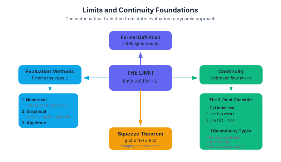
Calculus is often described as the mathematics of change, but before we can quantify change, we must quantify the "nearness" of values. In classical algebra, we deal with static values: $f(2)$ is exactly some number. In calculus, we ask a more sophisticated question: "As $x$ gets arbitrarily close to 2, what happens to $f(x)$?" This shift from static evaluation to dynamic approach is the birth of the Limit.
The Concept of the Limit
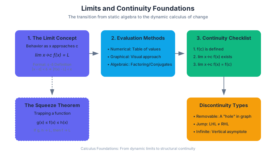
At its core, a limit describes the behavior of a function as its input approaches a specific value. We denote this as:
$$\lim_{x \to c} f(x) = L$$
This statement reads: "The limit of $f(x)$ as $x$ approaches $c$ equals $L$." Crucially, the limit is concerned with the neighborhood of $c$, not the value of $f(c)$ itself. In fact, $f(c)$ might be undefined, yet the limit can still exist.
Formal Definition ($\epsilon$-$\delta$)
To a mathematician, "arbitrarily close" is too vague. The formal definition, provided by Cauchy and Weierstrass, is the $\epsilon$-$\delta$ definition:
The limit of $f(x)$ as $x$ approaches $c$ is $L$ if, for every $\epsilon > 0$, there exists a $\delta > 0$ such that if $0 < |x - c| < \delta$, then $|f(x) - L| < \epsilon$.
This means if you pick a tiny distance $\epsilon$ from the target $L$, I can find a tiny distance $\delta$ around $c$ such that every $x$ in that range (except possibly $c$ itself) maps to a value within $\epsilon$ of $L$.
Graphical and Numerical Estimation
Before diving into algebra, we often estimate limits using two primary methods:
- Numerical Estimation: Creating a table of values that "zoom in" on $c$ from both sides (e.g., 1.9, 1.99, 1.999 and 2.1, 2.01, 2.001).
- Graphical Estimation: Observing the height the graph approaches from the left and right.
| Method | Strengths | Weaknesses |
|---|---|---|
| Numerical | Intuitive, handles complex functions easily with a calculator. | Can be misleading if the function oscillates wildly (e.g., $\sin(1/x)$). |
| Graphical | Excellent for identifying jump discontinuities and asymptotes. | Imprecise; "looks like 2" might actually be 2.0001. |
| Algebraic | Provides exact, provable values. | Can be difficult for transcendental or non-elementary functions. |
Algebraic Evaluation Techniques
When direct substitution ($\text{plugging in } c$) results in an indeterminate form like $0/0$, we employ several strategies:
- Factoring: Canceling out the "problematic" term.
- Rationalization: Using conjugates to clear radicals.
- Simplification: Combining complex fractions.
Continuity at a Point
A function is continuous if its graph can be drawn without lifting your pencil. However, in technical terms, continuity is defined by the behavior of limits. Continuity at a point $x = c$ requires three strict conditions to be met.
The Three-Point Checklist
A function $f(x)$ is continuous at $x = c$ if and only if:
- $f(c)$ is defined ($c$ is in the domain).
- $\lim_{x \to c} f(x)$ exists (left-hand limit = right-hand limit).
- $\lim_{x \to c} f(x) = f(c)$ (the limit matches the actual value).
Types of Discontinuity
If any of the three conditions above fail, the function is discontinuous. We classify these failures into three categories:
| Discontinuity Type | Description | Removability |
|---|---|---|
| Removable (Hole) | The limit exists, but $f(c)$ is undefined or different from the limit. | Removable: Can be fixed by redefining a single point. |
| Jump | The left-hand and right-hand limits exist but are not equal. | Non-removable: Common in piecewise functions. |
| Infinite | The function approaches $\pm\infty$ as $x \to c$. | Non-removable: Occurs at vertical asymptotes. |
Continuity on an Interval
A function is continuous on an open interval $(a, b)$ if it is continuous at every point in the interval. For a closed interval $[a, b]$, we also require one-sided continuity at the endpoints:
- $\lim_{x \to a^+} f(x) = f(a)$
- $\lim_{x \to b^-} f(x) = f(b)$
The Squeeze Theorem
Sometimes, a limit is too complex to evaluate directly (e.g., $\lim_{x \to 0} x^2 \sin(1/x)$). The Squeeze Theorem (also known as the Sandwich Theorem) allows us to find the limit of a "difficult" function by trapping it between two "easier" functions.
The Theorem
If $g(x) \le f(x) \le h(x)$ for all $x$ in an interval around $c$ (except possibly at $c$), and if: $$\lim_{x \to c} g(x) = \lim_{x \to c} h(x) = L$$ Then: $$\lim_{x \to c} f(x) = L$$
Classic Proof: The Limit of (sin x) / x
One of the most important applications of the Squeeze Theorem is proving that $\lim_{x \to 0} \frac{\sin x}{x} = 1$. This limit is the foundation for the derivatives of all trigonometric functions.
/* Mathematical Derivation of the Squeeze for sin(x)/x */

1. Consider a unit circle with angle x (in radians).
2. By comparing areas of the inner triangle, the sector, and the outer triangle:
   (1/2)sin(x) < (1/2)x < (1/2)tan(x)

3. Multiply by 2 and divide by sin(x):
   1 < x/sin(x) < 1/cos(x)

4. Take the reciprocal (flipping the inequalities):
   cos(x) < sin(x)/x < 1

5. Apply the limit as x -> 0:
   lim(x->0) cos(x) = 1
   lim(x->0) 1 = 1

6. Therefore, by Squeeze Theorem:
   lim(x->0) sin(x)/x = 1
Intermediate Value Theorem (IVT)
The Intermediate Value Theorem is an "existence theorem." It doesn't tell you where a value is, but it guarantees that a value must exist.
The Theorem
If $f$ is continuous on the closed interval $[a, b]$, and $k$ is any number between $f(a)$ and $f(b)$, then there exists at least one number $c$ in $[a, b]$ such that $f(c) = k$.
Why It Matters
The IVT is the mathematical justification for why, if you are 5 feet tall at age 10 and 6 feet tall at age 20, you must have been exactly 5.5 feet tall at some point in between. In engineering and computer science, the IVT is the basis for Bisection Methods used to find roots of equations.
Pitfall: The Continuity Requirement
The IVT only works if the function is continuous. If there is a jump discontinuity, the function can "skip" over the value $k$. Always verify continuity on the interval before applying the IVT.
Infinite Limits and Asymptotes
Limits also describe the "end behavior" of functions or their behavior near vertical barriers.
Vertical Asymptotes (Infinite Limits)
If $f(x)$ increases or decreases without bound as $x$ approaches $c$, we say the limit is infinite: $$\lim_{x \to c} f(x) = \infty \text{ or } -\infty$$ This indicates a vertical asymptote at $x = c$. This usually occurs when the denominator of a rational function is zero while the numerator is non-zero.
Horizontal Asymptotes (Limits at Infinity)
To find the behavior of a function as $x$ grows very large ($x \to \infty$) or very small ($x \to -\infty$), we look for horizontal asymptotes.
For a rational function $f(x) = \frac{P(x)}{Q(x)}$:
| Degree Comparison | Horizontal Asymptote |
|---|---|
| Degree of P < Degree of Q | $y = 0$ (The x-axis) |
| Degree of P = Degree of Q | $y = \frac{\text{leading coefficient of P}}{\text{leading coefficient of Q}}$ |
| Degree of P > Degree of Q | No horizontal asymptote (approaches $\pm\infty$ or slant asymptote) |
Common Pitfalls in Limits and Continuity
- Confusing "Limit Exists" with "Continuous": A limit can exist at a hole, but the function is not continuous there. Continuity requires the point to actually "fill" the hole.
- Ignoring One-Sided Limits: For a two-sided limit to exist, the left and right limits must be equal. If they differ by even an infinitesimal amount, the limit Does Not Exist (DNE).
- Algebraic Errors with Conjugates: When rationalizing, students often forget to distribute the negative sign when multiplying $(a - \sqrt{b})(a + \sqrt{b}) = a^2 - b$.
- Misapplying IVT: Using the IVT on an interval where the function has a vertical asymptote. The IVT requires continuity on the entire closed interval.
- Assuming $1/0 = \infty$: While $1/x$ approaches $\infty$ from the right, it approaches $-\infty$ from the left. Therefore, $\lim_{x \to 0} 1/x$ is DNE, not $\infty$.
Summary of Foundations
The study of limits and continuity is the process of formalizing "approach." By defining how functions behave near points and at the boundaries of their domains, we create the necessary framework for the Derivative (the limit of a difference quotient) and the Integral (the limit of a Riemann sum).
Source Materials
Study AP/College Calculus AB on Lykke
This course page is free to open: signed out, you can read its first two sections, and signing in, on any plan, opens the rest. The free Lykke Chrome extension syncs your own Canvas courses, so ChatGPT, Claude and Muse can answer from your classes and deadlines. It only reads Canvas.
Add the free extensionSign in to open every sectionAll sections of AP/College Calculus AB · Browse more course pages