From the free course AP/College Calculus AB on Lykke
Differential Equations and Modeling
Key concepts: Slope Fields · Separation of Variables · General vs. Particular Solutions · Exponential Growth and Decay · Initial Conditions
Solving equations that involve derivatives and modeling growth and decay.
Differential Equations and Modeling
In the study of calculus, we often focus on the relationship between a function and its instantaneous rate of change. However, in the real world—from the cooling of a cup of coffee to the spread of a viral pathogen—we rarely start with a clean function. Instead, we start with a relationship: an observation of how a system changes relative to its current state. This is the domain of Differential Equations (DEs).
A differential equation is, at its simplest, an equation involving a function and one or more of its derivatives. Solving a differential equation means finding the original function (or family of functions) that satisfies the stated relationship. This section explores the visual, analytical, and modeling techniques required to navigate these foundational tools of modern science and engineering.
The Anatomy of Differential Equations
Before diving into solutions, we must categorize the types of equations we encounter. In a first-year calculus context, we primarily focus on First-Order Ordinary Differential Equations (ODEs). These involve only the first derivative, $dy/dx$, and a single independent variable.
General vs. Particular Solutions
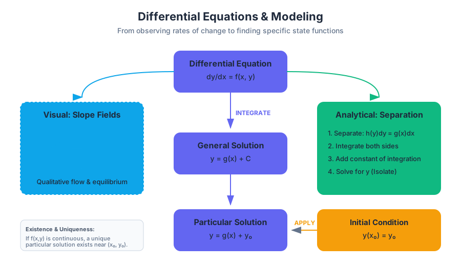
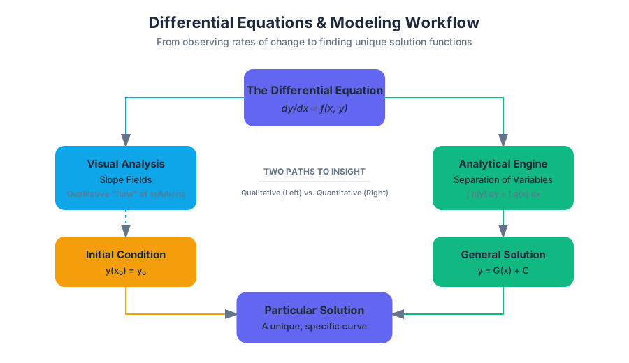
When we integrate a differential equation, we introduce a constant of integration, $C$. This results in a General Solution, which represents an infinite family of curves. Each curve in the family shares the same derivative property but is shifted or scaled.
To narrow this down to a single, unique curve, we require an Initial Condition—a specific point $(x_0, y_0)$ through which the solution must pass. Applying this condition allows us to solve for $C$, yielding the Particular Solution.
| Concept | Definition | Mathematical Form | Result Type |
|---|---|---|---|
| Differential Equation | An equation relating $y, x,$ and $dy/dx$. | $dy/dx = f(x, y)$ | A relationship |
| General Solution | The set of all possible functions satisfying the DE. | $y = g(x) + C$ | A family of curves |
| Initial Condition | A known point on the solution curve. | $y(x_0) = y_0$ | A constraint |
| Particular Solution | The specific function satisfying both the DE and the initial condition. | $y = g(x) + 5$ | A single curve |
The Existence and Uniqueness Theorem: For a first-order DE $dy/dx = f(x, y)$, if $f$ and its partial derivative with respect to $y$ are continuous near a point $(x_0, y_0)$, then there exists a unique particular solution passing through that point.
Slope Fields: Visualizing the Derivative
When an analytical solution is difficult or impossible to find, we turn to qualitative analysis. A Slope Field (or direction field) is a graphical representation of a differential equation. Since $dy/dx$ represents the slope of the tangent line at any point $(x, y)$, we can draw short line segments at various points in the Cartesian plane to visualize the "flow" of the solutions.
Construction and Interpretation
To construct a slope field for $dy/dx = f(x, y)$:
- Select a grid of points $(x, y)$.
- Calculate the value of the derivative at each point.
- Draw a short line segment with that calculated slope at each point.
By looking at a slope field, we can identify Equilibrium Solutions (where $dy/dx = 0$), see where solutions are increasing or decreasing, and observe the Concavity of the solution curves.
Separation of Variables: The Analytical Engine
Separation of Variables is the primary algebraic technique for solving first-order differential equations. It is applicable when the derivative can be expressed as a product of a function of $x$ and a function of $y$: $$\frac{dy}{dx} = g(x)h(y)$$
The Algorithm
To solve via separation, follow these rigorous steps:
| Step | Action | Mathematical Operation |
|---|---|---|
| 1 | Separate | Move all $y$ terms (including $dy$) to one side and $x$ terms (including $dx$) to the other. |
| 2 | Integrate | Perform indefinite integration on both sides. |
| 3 | Constant | Add the constant of integration $+C$ (usually on the $x$-side). |
| 4 | Solve for $y$ | Use algebra to isolate $y$ (the General Solution). |
| 5 | Apply IC | If an initial condition is given, solve for $C$ (the Particular Solution). |
Worked Example: Solving a Separable Equation
Find the particular solution for $\frac{dy}{dx} = \frac{x^2}{y}$ given the initial condition $y(0) = 2$.
\begin{aligned}
\text{1. Separate variables: } & y \, dy = x^2 \, dx \\
\text{2. Integrate both sides: } & \int y \, dy = \int x^2 \, dx \\
\text{3. Result of integration: } & \frac{1}{2}y^2 = \frac{1}{3}x^3 + C \\
\text{4. Solve for General Solution: } & y^2 = \frac{2}{3}x^3 + C_1 \implies y = \pm\sqrt{\frac{2}{3}x^3 + C_1} \\
\text{5. Apply Initial Condition } (0, 2): & 2 = \sqrt{\frac{2}{3}(0)^3 + C_1} \implies 2 = \sqrt{C_1} \implies C_1 = 4 \\
\text{6. Particular Solution: } & y = \sqrt{\frac{2}{3}x^3 + 4}
\end{aligned}
Warning: Always add the constant $C$ immediately after integrating. Adding it at the very end of the algebraic manipulation is a common error that leads to incorrect particular solutions.
Exponential Growth and Decay Models
One of the most significant applications of differential equations is modeling quantities that change at a rate proportional to their current size. This is described by the equation: $$\frac{dy}{dt} = ky$$ where $k$ is the growth constant ($k > 0$) or decay constant ($k < 0$).
Derivation of the Law of Exponential Change
We can derive the standard growth formula using separation of variables:
DERIVATION: dy/dt = ky
-----------------------
1. Separate: (1/y) dy = k dt
2. Integrate: ∫ (1/y) dy = ∫ k dt
3. Compute: ln|y| = kt + C
4. Exponentiate: |y| = e^(kt + C)
5. Simplify: |y| = e^C * e^(kt)
6. Let A = ±e^C: y(t) = A * e^(kt)

At t=0, y(0) = A * e^0 = A.
Therefore, A is the initial amount (y₀).

FINAL FORM: y(t) = y₀ * e^(kt)
Real-World Applications
Exponential models appear across diverse fields. The behavior is determined entirely by the sign and magnitude of $k$.
| Application | Equation Variant | Context |
|---|---|---|
| Population Growth | $dP/dt = kP$ | Unconstrained biological growth. |
| Radioactive Decay | $dm/dt = -km$ | The rate of decay is proportional to the mass remaining. |
| Newton's Law of Cooling | $dT/dt = -k(T - T_s)$ | Rate of temp change is proportional to the difference with surroundings. |
| Continuous Interest | $dA/dt = rA$ | Financial modeling of continuously compounded accounts. |
Newton's Law of Cooling: A Case Study
Newton's Law of Cooling states that the rate of change of the temperature $T$ of an object is proportional to the difference between its temperature and the ambient temperature $T_s$. $$\frac{dT}{dt} = -k(T - T_s)$$ This is a separable DE. If we let $u = T - T_s$, then $du/dt = dT/dt$, and the equation simplifies to $du/dt = -ku$, which we already know results in $u(t) = u_0 e^{-kt}$. Substituting back: $$T(t) = T_s + (T_0 - T_s)e^{-kt}$$
Numerical Methods: When Algebra Fails
Not all differential equations are separable. For equations like $dy/dx = x + y$, we cannot isolate variables. In these cases, we use numerical approximation. The most fundamental method is Euler's Method.
Euler's Method uses the slope at a point to predict the next point a small distance $\Delta x$ (step size $h$) away. $$y_{n+1} = y_n + f(x_n, y_n) \cdot h$$
Common Pitfalls and Advanced Nuances
Even experienced practitioners encounter friction when modeling with DEs. Mastery requires recognizing these subtle traps.
1. The Absolute Value Trap
When integrating $1/y$, the result is $\ln|y|$. If the initial condition $y_0$ is negative, the absolute value is crucial.
- If $y > 0$, then $y = e^{kt+C}$.
- If $y < 0$, then $y = -e^{kt+C}$. The sign of the initial condition determines which branch of the solution you are on.
2. Domain of Validity
A particular solution is only valid on the continuous interval containing the initial condition. If the solution $y(x)$ has a vertical asymptote (e.g., $y = 1/(1-x)$), and your initial condition is at $x=0$, the solution is only valid for $x < 1$.
3. Misinterpreting Slope Fields
Students often confuse the slope field of $dy/dx = f(x)$ with $dy/dx = f(y)$.
- If $dy/dx$ depends only on $x$, all segments in a vertical column are parallel.
- If $dy/dx$ depends only on $y$ (Autonomous Equation), all segments in a horizontal row are parallel.
4. The $+C$ Placement
In separation of variables, $C$ represents the accumulation of constants from both sides. It must be present before you perform algebraic operations like exponentiation or square roots.
- Correct: $\ln|y| = x + C \implies y = e^{x+C} = Ce^x$
- Incorrect: $\ln|y| = x \implies y = e^x \implies y = e^x + C$
Summary of Modeling Workflow
To model a physical system using differential equations, follow this pipeline:
- Identify the Rate: Determine what $dy/dt$ represents (e.g., velocity, rate of decay).
- Formulate the Equation: Translate the physical description into math (e.g., "rate is proportional to..." $\to dy/dt = ky$).
- Choose a Method:
- Can variables be separated? Use Separation of Variables.
- Is it a standard growth/decay model? Use $y = y_0 e^{kt}$.
- Is it complex? Use Slope Fields or Numerical Methods.
- Solve for $C$: Use the initial state of the system.
- Interpret: Ensure the limits of the function make sense (e.g., population shouldn't go to infinity if there's a carrying capacity).
Source Materials
Study AP/College Calculus AB on Lykke
This course page is free to open: signed out, you can read its first two sections, and signing in, on any plan, opens the rest. The free Lykke Chrome extension syncs your own Canvas courses, so ChatGPT, Claude and Muse can answer from your classes and deadlines. It only reads Canvas.
Add the free extensionSign in to open every sectionAll sections of AP/College Calculus AB · Browse more course pages