From the free course AP/College Calculus AB on Lykke
Analytical Applications of Differentiation
Key concepts: Mean Value Theorem (MVT) · Extreme Value Theorem (EVT) · First and Second Derivative Tests · Concavity and Inflection Points · Optimization Problems
Using derivatives to analyze function behavior, including extrema, concavity, and optimization.
Analytical Applications of Differentiation
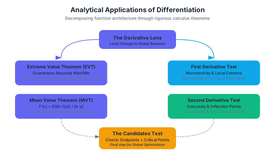
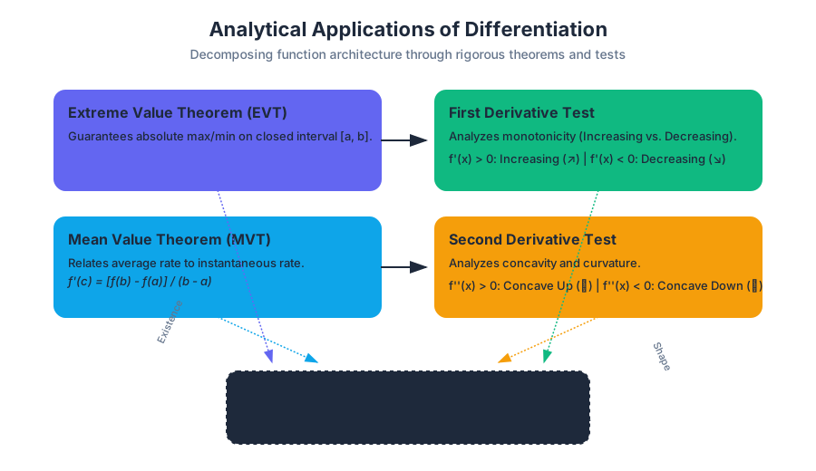
The study of differentiation extends far beyond the mere calculation of slopes. In the analytical realm, the derivative serves as a high-resolution lens through which we can decompose the behavior of functions, predict their long-term trajectories, and find optimal solutions to complex physical and economic problems. This section explores the rigorous theorems and tests that allow us to move from a local understanding of change to a global understanding of function architecture.
The Extreme Value Theorem (EVT)
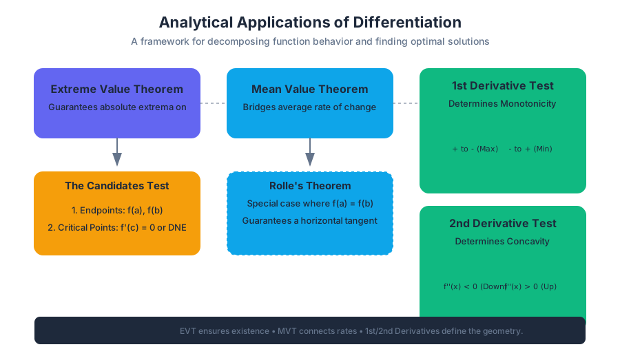
The Extreme Value Theorem (EVT) is an existence theorem. It does not tell us where a maximum or minimum occurs, but it guarantees that under specific conditions, they must exist. This is the logical bedrock upon which all optimization is built.
The Extreme Value Theorem: If a function $f$ is continuous on a closed interval $[a, b]$, then $f$ must attain an absolute maximum and an absolute minimum at least once within that interval.
Why It Matters
In real-world engineering, we often operate within "constraints" (the closed interval). If you are designing a bridge, there is a maximum load it will face. If you are a chemist, there is a specific temperature range for a reaction. The EVT ensures that within these bounds, there is a "best" and "worst" case scenario to find.
The Candidates Test
To find these absolute extrema, we use the Candidates Test. We check the function values at:
- Critical Points: Where $f'(x) = 0$ or $f'(x)$ is undefined.
- Endpoints: The boundaries $a$ and $b$ of the interval.
| Feature | Absolute Extrema | Relative (Local) Extrema |
|---|---|---|
| Definition | The highest/lowest point on the entire domain/interval. | A point higher/lower than all nearby points. |
| Existence | Guaranteed on closed intervals by EVT. | Not guaranteed; depends on function shape. |
| Location | Can be at critical points OR endpoints. | Must be at critical points. |
| Requirement | $f(c) \geq f(x)$ for all $x$ in domain. | $f(c) \geq f(x)$ for $x$ in an open interval near $c$. |
The Mean Value Theorem (MVT)
If the EVT is about "where we are," the Mean Value Theorem (MVT) is about "how we got there." It bridges the gap between the average rate of change (algebra) and the instantaneous rate of change (calculus).
The Mean Value Theorem: If $f$ is continuous on $[a, b]$ and differentiable on $(a, b)$, then there exists at least one point $c$ in $(a, b)$ such that: $$f'(c) = \frac{f(b) - f(a)}{b - a}$$
The "Speed Trap" Analogy
Imagine you enter a toll road at 1:00 PM and exit 100 miles later at 2:00 PM. Your average speed was 100 mph. Even if a police officer didn't see you speeding, the MVT proves that at some specific moment $c$ between 1:00 and 2:00, your speedometer read exactly 100 mph.
Rolle's Theorem: A Special Case
Rolle's Theorem is a specific instance of the MVT where $f(a) = f(b)$. If you start and end at the same height, and the function is "smooth" (differentiable), there must be at least one point where the tangent line is horizontal ($f'(c) = 0$).
\begin{aligned}
&\text{Proof Sketch of MVT using Rolle's Theorem:} \\
&\text{1. Define a secant line equation: } g(x) = f(a) + \frac{f(b)-f(a)}{b-a}(x-a) \\
&\text{2. Create an auxiliary function: } h(x) = f(x) - g(x) \\
&\text{3. Note that } h(a) = 0 \text{ and } h(b) = 0. \\
&\text{4. By Rolle's Theorem, } \exists c \in (a, b) \text{ such that } h'(c) = 0. \\
&\text{5. } h'(x) = f'(x) - \frac{f(b)-f(a)}{b-a} \implies f'(c) = \frac{f(b)-f(a)}{b-a}.
\end{aligned}
Monotonicity and the First Derivative Test
To understand the "flow" of a function, we examine the sign of its first derivative. This allows us to categorize intervals of increase and decrease and identify local extrema.
Critical Points
A Critical Point occurs at $x = c$ if $f'(c) = 0$ or if $f'(c)$ does not exist. These are the only locations where a function can potentially change from increasing to decreasing.
The First Derivative Test
This test classifies critical points based on the behavior of $f'(x)$ as it "crosses" the point.
| Sign Change of $f'(x)$ | Conclusion at $x = c$ | Visual Interpretation |
|---|---|---|
| Positive to Negative | Local Maximum | A mountain peak ($\nearrow \bullet \searrow$) |
| Negative to Positive | Local Minimum | A valley floor ($\searrow \bullet \nearrow$) |
| No sign change | No Extremum | A "shelf" or point of inflection ($y=x^3$ at $x=0$) |
Concavity and the Second Derivative Test
While the first derivative tells us the direction of a function, the second derivative $f''(x)$ tells us the Concavity—the way the function curves.
Concavity Definitions
- Concave Up ($f''(x) > 0$): The function is shaped like a cup ($\cup$). The slopes are increasing.
- Concave Down ($f''(x) < 0$): The function is shaped like a frown ($\cap$). The slopes are decreasing.
- Inflection Point: A point where the concavity changes (e.g., from up to down). This occurs where $f''(x) = 0$ or is undefined, and the sign of $f''(x)$ actually changes.
The Second Derivative Test
This is an alternative way to classify critical points. If $f'(c) = 0$:
- If $f''(c) > 0$, then $f$ has a local minimum at $c$.
- If $f''(c) < 0$, then $f$ has a local maximum at $c$.
- If $f''(c) = 0$, the test is inconclusive (use the First Derivative Test).
Global Optimization and Applied Modeling
Optimization is the process of finding the maximum or minimum value of a "target" function (the objective function) subject to certain constraints.
The Optimization Workflow
- Identify Variables: Determine what can be changed (e.g., $x$ for width, $y$ for height).
- Primary Equation: Write the formula for the quantity to be optimized (e.g., Area $A = xy$).
- Secondary Equation (Constraint): Use given info to relate variables (e.g., Perimeter $2x + 2y = 100$).
- Substitution: Reduce the primary equation to a single variable using the constraint.
- Differentiation: Find the derivative and set to zero to find critical points.
- Verification: Use the First or Second Derivative test to ensure it's the desired extremum.
Worked Example: The Maximum Volume Box
A sheet of cardboard 20in by 20in has squares of side $x$ cut out of the corners to form an open-top box. Find the value of $x$ that maximizes volume.
- Volume: $V(x) = (20 - 2x)(20 - 2x)x = 4x^3 - 80x^2 + 400x$
- Domain: $x \in [0, 10]$ (since $2x$ cannot exceed 20).
- Derivative: $V'(x) = 12x^2 - 160x + 400$
- Solve $V'(x) = 0$: $4(3x^2 - 40x + 100) = 0 \implies 4(3x - 10)(x - 10) = 0$.
- Critical Points: $x = 10/3$ and $x = 10$.
- Test: $V(10) = 0$ (minimum). $V(10/3) \approx 592.6$ in³.
- Result: The optimal cut is $3.33$ inches.
Common Pitfalls and Edge Cases
Analytical differentiation is rigorous, but several "traps" exist for the unwary student or engineer.
- The $f''(c) = 0$ Trap: Many assume if the second derivative is zero, it's an inflection point. Consider $f(x) = x^4$. At $x=0$, $f''(0) = 0$, but the function is concave up on both sides. No inflection occurs.
- Endpoint Neglect: In absolute extrema problems on $[a, b]$, the maximum is frequently at $a$ or $b$, not at a critical point. Always check the boundaries.
- Differentiability Requirements: The MVT requires the function to be differentiable on the open interval. A function like $f(x) = |x|$ on $[-1, 1]$ is continuous, but because it has a "corner" at $x=0$, the MVT does not apply.
- Implicit Relations: When dealing with relations like $x^2 + y^2 = 25$, finding extrema requires implicit differentiation or conversion to polar coordinates. The "slope" can be vertical, making $dy/dx$ undefined.
| Error | Consequence | Prevention |
|---|---|---|
| Forgetting Endpoints | Missing the Global Maximum. | Always evaluate $f(a)$ and $f(b)$. |
| Assuming $f'(c)=0$ is a Max/Min | Misidentifying a Saddle Point. | Use the First Derivative Test sign chart. |
| Ignoring Domain Constraints | Finding a "solution" that is physically impossible. | Define the interval $[a, b]$ before differentiating. |
| Confusing $f'$ and $f''$ | Mixing up "increasing" with "concave up". | Remember: $f'$ is velocity, $f''$ is acceleration. |
Summary of Analytical Methods
To master the analytical applications of differentiation, one must view the first and second derivatives as a hierarchy of information.
- Function $f(x)$: Gives position/value.
- Derivative $f'(x)$: Gives direction (increasing/decreasing) and identifies potential turning points.
- Second Derivative $f''(x)$: Gives curvature (concavity) and identifies the "acceleration" of the slope.
By combining these, we can sketch any function with near-perfect accuracy and solve optimization problems that drive modern technology, from machine learning gradient descent to aerospace trajectory planning.
Source Materials
Study AP/College Calculus AB on Lykke
This course page is free to open: signed out, you can read its first two sections, and signing in, on any plan, opens the rest. The free Lykke Chrome extension syncs your own Canvas courses, so ChatGPT, Claude and Muse can answer from your classes and deadlines. It only reads Canvas.
Add the free extensionSign in to open every sectionAll sections of AP/College Calculus AB · Browse more course pages