From the free course 14 01 Principles Of Microeconomics Fall 2018 on Lykke
Supply, Demand, and Market Equilibrium
Key concepts: Law of Demand · Law of Supply · Market Equilibrium · Elasticity · Consumer and Producer Surplus
This section introduces the core framework of microeconomics: the supply and demand model. It covers how markets reach equilibrium and how changes in market conditions affect prices and quantities.
Supply, Demand, and Market Equilibrium
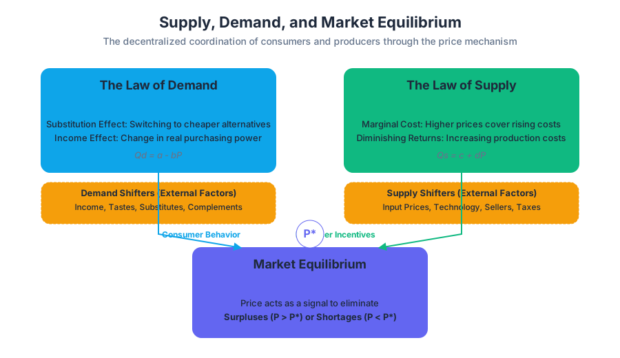
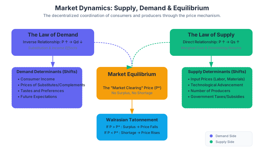
The supply and demand model is the fundamental analytical framework of microeconomics. It functions as a decentralized information-processing system, where prices act as signals that coordinate the independent actions of millions of consumers and producers. Rather than requiring a central planner to allocate resources, the market uses the price mechanism to reach an Equilibrium—a state where the quantity of goods buyers are willing to purchase matches the quantity sellers are willing to provide.
The Law of Demand
The Law of Demand states that, ceteris paribus (all other things being equal), there is an inverse relationship between the price of a good and the quantity demanded. As the price ($P$) increases, the quantity demanded ($Q_d$) decreases.
The Mechanics of Demand
This inverse relationship is driven by two primary economic phenomena:
- The Substitution Effect: As the price of a good rises, it becomes relatively more expensive compared to other goods. Consumers will naturally pivot toward cheaper substitutes to maintain their utility.
- The Income Effect: A price increase effectively reduces a consumer's purchasing power. Even if they do not switch to a substitute, they can afford less of the good than before.
Mathematically, a linear demand function is often represented as: $$Q_d = a - bP$$ Where $a$ represents the quantity demanded when price is zero (the horizontal intercept), and $b$ represents the slope of the demand curve (the sensitivity of quantity to price).
Shifts vs. Movements
It is a common pedagogical pitfall to confuse a movement along the demand curve with a shift of the demand curve.
- Movement: Caused solely by a change in the price of the good itself.
- Shift: Caused by a change in external factors (determinants).
| Determinant | Effect on Demand Curve | Example |
|---|---|---|
| Income (Normal Good) | Increase shifts curve Right | A raise leads to more dining out. |
| Income (Inferior Good) | Increase shifts curve Left | A raise leads to buying less instant ramen. |
| Price of Substitutes | Increase shifts curve Right | If coffee prices spike, tea demand rises. |
| Price of Complements | Increase shifts curve Left | If printer prices spike, ink demand falls. |
| Tastes/Preferences | Positive change shifts curve Right | A health study praising kale increases demand. |
| Expectations | Expected future price rise shifts curve Right | Buying gas today because a hike is expected tomorrow. |
The Law of Supply
The Law of Supply posits a direct relationship between price and quantity supplied ($Q_s$). As the market price increases, firms are incentivized to produce more because the marginal revenue of selling an additional unit exceeds the marginal cost of production for a larger range of output.
The Marginal Cost Derivation
In a competitive market, a firm's supply curve is essentially its Marginal Cost (MC) curve above the average variable cost. Because of the Law of Diminishing Marginal Returns, producing additional units eventually becomes more expensive (e.g., overtime pay for workers, wear and tear on machinery). Therefore, a higher price is required to justify the higher cost of producing those incremental units.
The linear supply function is typically expressed as: $$Q_s = c + dP$$ Where $c$ is the quantity supplied at a price of zero, and $d$ represents the responsiveness of supply to price changes.
Determinants of Supply
Just as with demand, supply can shift due to external factors:
| Factor | Effect on Supply Curve | Technical Reason |
|---|---|---|
| Input Prices | Increase shifts curve Left | Higher costs reduce profit margins per unit. |
| Technology | Improvement shifts curve Right | Increases productivity; lowers marginal cost. |
| Number of Sellers | Increase shifts curve Right | Aggregate market supply is the sum of individual supplies. |
| Expectations | Expected future price rise shifts curve Left | Firms may hoard inventory to sell at higher future prices. |
| Subsidies/Taxes | Subsidy shifts Right; Tax shifts Left | Effectively lowers or raises the cost of production. |
Market Equilibrium
Market Equilibrium occurs at the price ($P^*$) where $Q_d = Q_s$. At this point, the market "clears"—there is no excess supply (surplus) and no excess demand (shortage).
The Walrasian Tatonnement
In theory, markets reach equilibrium through a process called tatonnement ("groping"). If the current price is above equilibrium, a surplus exists. Sellers, unable to move their inventory, will lower prices to attract buyers. Conversely, if the price is below equilibrium, a shortage occurs. Buyers, unable to find the product, will bid prices up.
Solving for Equilibrium: A Worked Example
Consider a market with the following functions:
- Demand: $Q_d = 100 - 2P$
- Supply: $Q_s = 20 + 2P$
To find the equilibrium, set $Q_d = Q_s$: $$100 - 2P = 20 + 2P$$ $$80 = 4P$$ $$P^* = 20$$
Substitute $P^$ back into either equation to find $Q^$: $$Q^* = 100 - 2(20) = 60$$
Elasticity
Elasticity measures the responsiveness of one variable to changes in another. While the slope of a curve tells us the absolute change, elasticity provides a percentage-based, unitless measure.
Price Elasticity of Demand (PED)
PED measures how much the quantity demanded responds to a change in price: $$\epsilon_d = \frac{% \Delta Q_d}{% \Delta P}$$
Because demand curves are downward sloping, PED is technically negative, but economists often discuss it in absolute terms.
The Midpoint Method
To avoid different results when calculating elasticity between two points (depending on the direction of the change), the Midpoint Formula is used: $$\epsilon = \frac{(Q_2 - Q_1) / [(Q_2 + Q_1) / 2]}{(P_2 - P_1) / [(P_2 + P_1) / 2]}$$
Classification of Elasticity
| Value of $|\epsilon|$ | Classification | Meaning | | :--- | :--- | :--- | | $|\epsilon| > 1$ | Elastic | Quantity changes more than price (sensitive). | | $|\epsilon| < 1$ | Inelastic | Quantity changes less than price (insensitive). | | $|\epsilon| = 1$ | Unit Elastic | Quantity and price change by the same percentage. | | $|\epsilon| = 0$ | Perfectly Inelastic | Quantity does not change regardless of price (e.g., insulin). | | $|\epsilon| = \infty$ | Perfectly Elastic | Any price increase drops quantity to zero (commodities). |
\text{Derivation of Point Elasticity:} \\
\epsilon = \frac{dQ}{dP} \times \frac{P}{Q} \\
\text{For a demand curve } Q = a - bP, \text{ the derivative } \frac{dQ}{dP} = -b. \\
\text{Thus, } \epsilon = -b \left( \frac{P}{a - bP} \right).
Consumer and Producer Surplus
Equilibrium is not just a point of stability; it is the point that maximizes Total Surplus, the sum of benefits to all market participants.
Consumer Surplus (CS)
Consumer surplus is the difference between what a consumer is willing to pay (their reservation price) and what they actually pay. Graphically, it is the area below the demand curve and above the equilibrium price. $$CS = \int_{0}^{Q^} (P_{demand}(Q) - P^) dQ$$
Producer Surplus (PS)
Producer surplus is the difference between the market price and the marginal cost of production. It represents the benefit to sellers for participating in the market. Graphically, it is the area above the supply curve and below the equilibrium price. $$PS = \int_{0}^{Q^} (P^ - P_{supply}(Q)) dQ$$
Total Surplus and Efficiency
Total Surplus (TS) = CS + PS. An allocation of resources that maximizes total surplus is said to be Pareto Efficient. If a market is prevented from reaching equilibrium (e.g., through a tax or price control), a Deadweight Loss (DWL) occurs—this is surplus that is lost to neither the consumer nor the producer, representing a net loss to society.
Comparative Statics: Analyzing Market Shocks
Economists use Comparative Statics to predict how equilibrium changes when a determinant shifts. This involves comparing the initial equilibrium to the new equilibrium after a shock.
The Four Laws of Supply and Demand
- Demand Increases ($\uparrow D$): $P^$ increases, $Q^$ increases.
- Demand Decreases ($\downarrow D$): $P^$ decreases, $Q^$ decreases.
- Supply Increases ($\uparrow S$): $P^$ decreases, $Q^$ increases.
- Supply Decreases ($\downarrow S$): $P^$ increases, $Q^$ decreases.
Ambiguous Cases (Double Shifts)
When both curves shift simultaneously, either the change in price or the change in quantity will be ambiguous unless the magnitudes of the shifts are known.
| Shift | $\uparrow$ Supply | $\downarrow$ Supply |
|---|---|---|
| $\uparrow$ Demand | $Q \uparrow$, $P$ Ambiguous | $P \uparrow$, $Q$ Ambiguous |
| $\downarrow$ Demand | $P \downarrow$, $Q$ Ambiguous | $Q \downarrow$, $P$ Ambiguous |
Common Pitfalls and Edge Cases
1. The Giffen Good
A rare exception to the Law of Demand where an increase in price causes an increase in quantity demanded. This occurs with highly inferior goods that make up a large portion of a poor consumer's budget. When the price rises, the "income effect" is so negative that the consumer can no longer afford better substitutes (like meat) and must buy more of the staple (like bread or potatoes) to survive.
2. Price Ceilings and Floors
Governments often intervene with price controls.
- Price Ceiling: A legal maximum price (e.g., rent control). If set below equilibrium, it causes a shortage.
- Price Floor: A legal minimum price (e.g., minimum wage). If set above equilibrium, it causes a surplus (unemployment).
3. Tax Incidence
The "burden" of a tax does not depend on who writes the check to the government. Instead, it depends on relative elasticities. The side of the market that is more inelastic (less responsive to price changes) will bear more of the tax burden.
Source Materials
Study 14 01 Principles Of Microeconomics Fall 2018 on Lykke
This course page is free to open: signed out, you can read its first two sections, and signing in, on any plan, opens the rest. The free Lykke Chrome extension syncs your own Canvas courses, so ChatGPT, Claude and Muse can answer from your classes and deadlines. It only reads Canvas.
Add the free extensionSign in to open every sectionAll sections of 14 01 Principles Of Microeconomics Fall 2018 · Browse more course pages