From the free course 14 01 Principles Of Microeconomics Fall 2018 on Lykke
Market Structures and Competition
Key concepts: Perfect Competition · Monopoly · Oligopoly · Game Theory · Nash Equilibrium
This section examines different types of market environments, ranging from perfectly competitive markets to monopolies and strategic oligopolies.
Market Structures and Competition
In neoclassical microeconomics, the behavior of a firm is not dictated solely by its internal production function, but by the external environment in which it operates. This environment, known as the Market Structure, determines the degree of pricing power a firm possesses, the barriers to entry for potential competitors, and the ultimate efficiency of resource allocation.
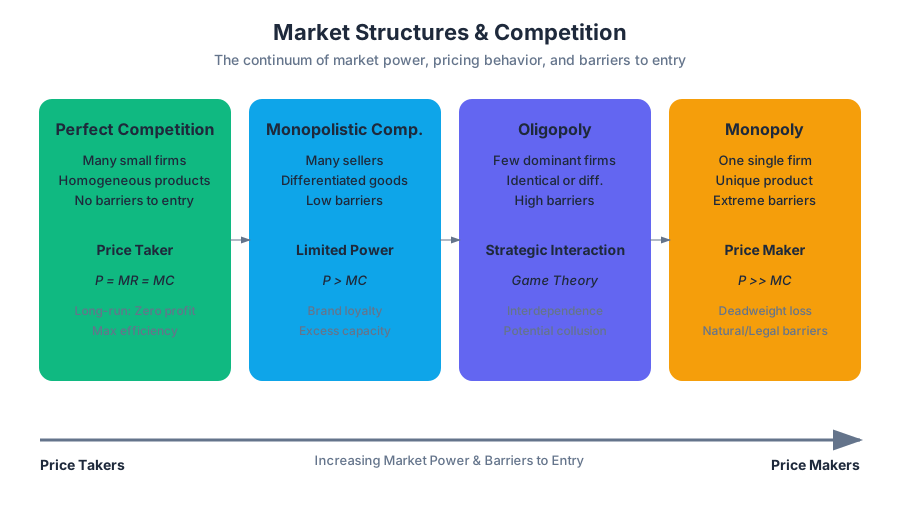
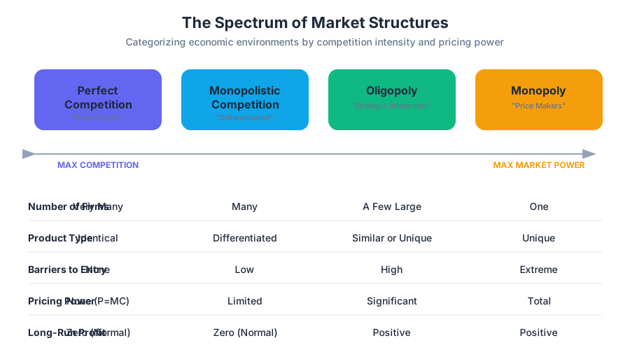
At one end of the spectrum lies Perfect Competition, a theoretical benchmark where firms are "price takers." At the other lies Monopoly, where a single firm wields total market power. Between these extremes are Oligopoly and Monopolistic Competition, where strategic interactions and product differentiation define the landscape. Understanding these structures requires a rigorous application of marginal analysis and, in the case of strategic interaction, Game Theory.
Perfect Competition
Perfect competition represents an idealized market state where the forces of supply and demand operate without friction. It serves as the baseline against which all other market "imperfections" are measured.
1. Characteristics and Assumptions
For a market to be considered perfectly competitive, four stringent criteria must be met:
- Large Number of Buyers and Sellers: No individual agent has a large enough market share to influence the equilibrium price.
- Homogeneous Products: The goods offered by different sellers are perfect substitutes. Consumers are indifferent between sellers.
- Perfect Information: All agents have complete knowledge of prices, technologies, and profit opportunities.
- Free Entry and Exit: There are no legal, technological, or financial barriers preventing firms from entering or leaving the industry in the long run.
2. The Firm's Decision: Price Taking
In this structure, the firm faces a perfectly elastic demand curve at the market price $P^*$. The firm's total revenue is $TR = P \cdot Q$, and because $P$ is constant, the Marginal Revenue (MR) is simply $P$.
The Profit Maximization Rule: To maximize profit $\pi$, a firm must produce at the quantity $Q$ where the cost of the last unit produced equals the revenue it generates: $$P = MC(Q)$$
3. Long-Run Equilibrium and the Zero-Profit Condition
In the short run, a firm may earn economic profits if $P > ATC$ (Average Total Cost). However, these profits signal an opportunity to outsiders. Due to the assumption of free entry, new firms will enter the market, shifting the industry supply curve to the right and driving down the price. This process continues until $P = \min(ATC)$, at which point Economic Profit is zero.
| Parameter | Short Run | Long Run |
|---|---|---|
| Profit ($\pi$) | Can be positive, zero, or negative | Must be zero (Normal Profit) |
| Price (P) | $P = MC$ | $P = MC = \min(ATC)$ |
| Efficiency | Allocative efficiency achieved | Allocative and Productive efficiency achieved |
| Firm Behavior | Adjusts $Q$ to $P$ | Enters/Exits based on $\pi$ |
Monopoly
A Monopoly exists when a single firm is the sole producer of a product with no close substitutes. Unlike the competitive firm, the monopolist is a "price maker."
1. Barriers to Entry
Monopolies persist only if other firms are prevented from entering. These barriers include:
- Ownership of Key Resources: (e.g., De Beers and diamonds).
- Government Franchises/Patents: Legal protections for intellectual property.
- Natural Monopolies: Occur when Economies of Scale are so significant that a single firm can supply the entire market at a lower cost than two or more firms could (e.g., water utilities).
2. The Math of Monopoly Power
The monopolist faces the downward-sloping market demand curve $P(Q)$. Consequently, to sell an additional unit, the firm must lower the price on all units sold. This implies that Marginal Revenue (MR) is always less than Price ($P$).
Derivation of Marginal Revenue: Let $TR = P(Q) \cdot Q$. $MR = \frac{d(TR)}{dQ} = P + Q \cdot \frac{dP}{dQ}$ Since $\frac{dP}{dQ} < 0$ for a downward sloping demand curve, $MR < P$.
3. The Lerner Index
The degree of monopoly power is often measured by the Lerner Index ($L$), which quantifies the markup over marginal cost.
L = \frac{P - MC}{P} = \frac{1}{|\epsilon_d|}
Where $\epsilon_d$ is the price elasticity of demand. This formula demonstrates that the less elastic the demand (smaller $\epsilon_d$), the greater the firm's ability to charge a price significantly above marginal cost.
4. Social Cost: Deadweight Loss
Monopolies are inefficient because they produce a quantity where $P > MC$. This results in Deadweight Loss (DWL)—a loss of total surplus (consumer + producer) that occurs because the firm restricts output to keep prices high.
| Feature | Perfect Competition | Monopoly |
|---|---|---|
| Quantity | $Q_{comp}$ where $P = MC$ | $Q_{mono}$ where $MR = MC$ |
| Price | $P = MC$ | $P > MC$ |
| Welfare | Maximizes Total Surplus | Creates Deadweight Loss |
| Long-run Profit | Zero | Can be positive |
Oligopoly
An Oligopoly is a market structure dominated by a small number of large firms. The defining characteristic of an oligopoly is Strategic Interdependence: the profit of one firm depends not only on its own actions but also on the actions of its rivals.
1. The Cournot Model (Quantity Competition)
In the Cournot model, firms simultaneously choose the quantity they will produce. Each firm treats the other's output as fixed. The equilibrium occurs at the intersection of the firms' Reaction Functions.
2. The Bertrand Model (Price Competition)
In the Bertrand model, firms compete on price. If products are homogeneous, consumers will always buy from the firm with the lowest price. This leads to a "race to the bottom" where $P = MC$, even with only two firms. This is known as the Bertrand Paradox.
3. Measuring Market Concentration: HHI
Regulators use the Herfindahl-Hirschman Index (HHI) to determine the competitiveness of an industry. It is calculated by squaring the market share of each firm.
- HHI < 1,500: Unconcentrated (Competitive).
- 1,500 < HHI < 2,500: Moderately Concentrated.
- HHI > 2,500: Highly Concentrated (Oligopolistic).
Game Theory and Nash Equilibrium
Because oligopolists must act strategically, we use Game Theory to model their behavior.
1. Components of a Game
A game consists of:
- Players: The decision-makers (firms).
- Strategies: The possible actions (e.g., High Price, Low Price).
- Payoffs: The outcomes (profits) resulting from the combination of strategies.
2. Nash Equilibrium
A Nash Equilibrium is a situation where each player chooses their best strategy, given the strategies chosen by the other players. No player has an incentive to deviate unilaterally.
Formal Definition: A strategy profile $(s^_i, s^{-i})$ is a Nash Equilibrium if for every player $i$: $$\pi_i(s^_i, s^{-i}) \geq \pi_i(s_i, s^*_{-i}) \quad \forall s_i \in S_i$$
3. The Prisoner's Dilemma in Business
Oligopolies often face a Prisoner's Dilemma. While both firms would earn higher profits by colluding (forming a Cartel) and keeping prices high, the individual incentive to "cheat" by lowering prices to capture the whole market often leads to a sub-optimal equilibrium for the firms.
| Firm A \ Firm B | Collude (High P) | Cheat (Low P) |
|---|---|---|
| Collude (High P) | ($10M, $10M) | ($2M, $15M) |
| Cheat (Low P) | ($15M, $2M) | ($5M, $5M) |
In this matrix, (Cheat, Cheat) is the Nash Equilibrium, even though (Collude, Collude) yields higher collective profits.
4. Repeated Games and Tit-for-Tat
In the real world, firms interact repeatedly. This allows for the development of "trigger strategies." In a Tit-for-Tat strategy, a firm cooperates in the first period and subsequently mimics the rival's previous move. This can sustain collusion without an explicit (and illegal) agreement.
Summary of Market Structures
| Feature | Perfect Competition | Monopolistic Competition | Oligopoly | Monopoly |
|---|---|---|---|---|
| Number of Firms | Many | Many | Few | One |
| Type of Product | Identical | Differentiated | Identical or Differentiated | Unique |
| Barriers to Entry | None | Low | High | Very High |
| Pricing Power | None (Price Taker) | Some | Substantial | Total (Price Maker) |
| Example | Wheat, Stocks | Restaurants, Clothing | Airlines, Soft Drinks | Local Utilities |
Common Pitfalls and Misconceptions
- "Monopolies can charge any price they want": False. Monopolists are still constrained by the demand curve. If they set the price too high, the quantity demanded drops to zero. They set the price to maximize $\pi$, not to maximize $P$.
- "Zero economic profit means the firm is failing": False. Economic profit includes Opportunity Cost. Zero economic profit means the firm's owners are earning exactly what they could have earned in their next best alternative (a "normal" return on investment).
- "Nash Equilibrium is always the best outcome": False. As seen in the Prisoner's Dilemma, the Nash Equilibrium is often Pareto-inefficient, meaning there is another outcome where at least one player is better off without making anyone else worse off.
Source Materials
Study 14 01 Principles Of Microeconomics Fall 2018 on Lykke
This course page is free to open: signed out, you can read its first two sections, and signing in, on any plan, opens the rest. The free Lykke Chrome extension syncs your own Canvas courses, so ChatGPT, Claude and Muse can answer from your classes and deadlines. It only reads Canvas.
Add the free extensionSign in to open every sectionAll sections of 14 01 Principles Of Microeconomics Fall 2018 · Browse more course pages