Spring 2026 - Math 354 - Sections 02/04
Institution: MIT
33 study materials · 9 sections
Math 354: Linear Optimization provides a comprehensive introduction to the mathematical theory and application of linear programming. The course covers the transition from foundational linear algebra concepts, such as matrix inversion and linear independence, to advanced optimization techniques including the Simplex method and Duality theory. Students learn to model real-world constraints, solve problems geometrically in two dimensions, and apply algebraic methods for higher-dimensional challenges. Assessment is conducted through a mastery-based grading system that emphasizes conceptual understanding and procedural accuracy.
Course Sections
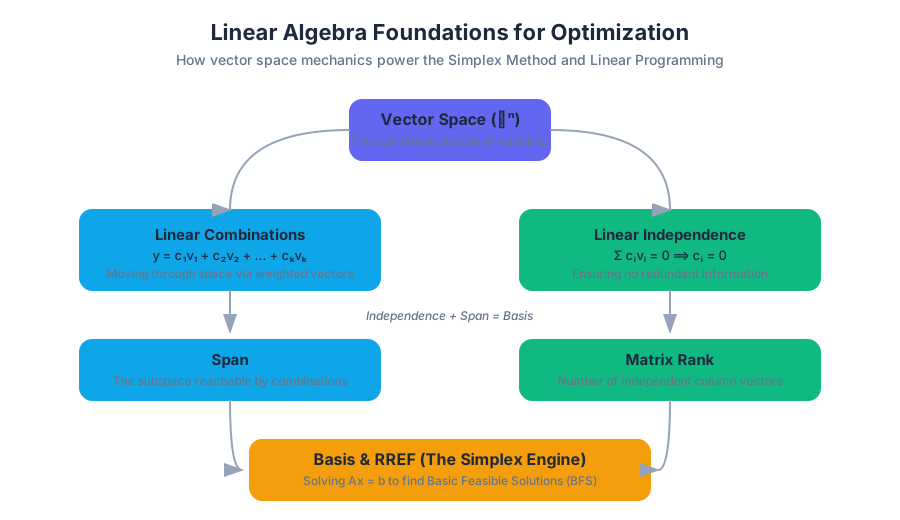
Linear Algebra Review and Matrix Operations
Key concepts: Reduced Row Echelon Form (RREF) · Matrix Inversion · Linear Independence · Linear Combinations · Vector Spaces
A foundational review of linear algebra techniques essential for optimization, focusing on matrix inversion and vector space properties.
Linear Algebra Review and Matrix Operations
Linear algebra is the mathematical language of optimization. While high-level solvers often abstract away the underlying arithmetic, a mastery of linear programming (LP) requires a profound understanding of how systems of linear equations are manipulated, how vector spaces are structured, and how matrix transformations define the feasible regions of our problems. In this article, we will move beyond basic definitions to explore the mechanics of matrix operations that power the Simplex method and other fundamental algorithms in operations research.
Vector Spaces and Linear Combinations
At the core of linear algebra lies the Vector Space. For the purposes of optimization and the Simplex method, we primarily concern ourselves with the real coordinate space $\mathbb{R}^n$. A vector space is not merely a collection of points; it is a set closed under two primary operations: vector addition and scalar multiplication.
The Geometry of Linear Combinations
A Linear Combination of a set of vectors ${v_1, v_2, \dots, v_k}$ is an expression of the form: $$y = c_1v_1 + c_2v_2 + \dots + c_kv_k$$ where $c_i$ are scalars. In the context of Linear Programming, every point within a feasible region can be viewed as a linear combination of the extreme points (vertices) of the constraint polytope, provided the weights $c_i$ satisfy specific conditions (such as non-negativity and summing to one for convex combinations).
Definition: Span The Span of a set of vectors is the set of all possible linear combinations of those vectors. If the span of a set of vectors in $\mathbb{R}^n$ covers the entire space, we say the set "spans" $\mathbb{R}^n$.
| Concept | Mathematical Representation | Geometric Interpretation |
|---|---|---|
| Vector | $x \in \mathbb{R}^n$ | A directed arrow or point in space. |
| Scalar Multiplication | $\alpha x$ | Scaling the length of the vector. |
| Linear Combination | $\sum c_i v_i$ | Reaching a new point by following weighted vectors. |
| Span | $\text{span}{v_1, \dots, v_k}$ | The "subspace" (line, plane, etc.) filled by the vectors. |
Implementation: Linear Combinations in Practice
In modern data science and engineering, we rarely perform these calculations by hand. However, understanding how a library like NumPy handles these operations is crucial for performance.
import numpy as np

# Defining vectors in R^4 (as seen in HW1_0-5-6a)
v1 = np.array([-1, 2, 4, 3])
v2 = np.array([3, -1, 2, 5])
v3 = np.array([-5, 5, 6, 1])

# Check if v3 is a linear combination of v1 and v2
# We solve the system: c1*v1 + c2*v2 = v3
# This is equivalent to Ac = b where A = [v1, v2] and b = v3
A = np.stack([v1, v2], axis=1)
try:
    # Use least squares to find coefficients
    c, residuals, rank, s = np.linalg.lstsq(A, v3, rcond=None)

    # If residuals are near zero, v3 is a linear combination
    is_linear_comb = np.allclose(A @ c, v3)
    print(f"Coefficients: {c}")
    print(f"Is v3 a linear combination? {is_linear_comb}")
except np.linalg.LinAlgError:
    print("System is inconsistent.")
Linear Independence
A set of vectors is Linearly Independent if no vector in the set can be expressed as a linear combination of the others. Formally, the set ${v_1, v_2, \dots, v_k}$ is linearly independent if the only solution to the vector equation: $$c_1v_1 + c_2v_2 + \dots + c_kv_k = 0$$ is the trivial solution $c_1 = c_2 = \dots = c_k = 0$.
Why Independence Matters in Optimization
In the Simplex method, we transform inequality constraints into equality constraints by adding slack variables. This results in a system $Ax = b$ where $A$ is an $m \times n$ matrix with $n > m$. To find a Basic Feasible Solution (BFS), we must select $m$ linearly independent columns from $A$ to form a Basis. If the columns were linearly dependent, the resulting basis matrix $B$ would be singular (non-invertible), and we could not solve for the basic variables.
Determining Independence via Rank
The Rank of a matrix is the maximum number of linearly independent column vectors in the matrix.
- If a set of $k$ vectors in $\mathbb{R}^n$ has rank $k$, they are linearly independent.
- If the rank is less than $k$, at least one vector is redundant.
Mathematical Derivation: Testing for Independence
To test if $S = {v_1, v_2, v_3}$ is linearly independent, we set up the augmented matrix $[v_1 v_2 v_3 | 0]$ and reduce it to RREF.
\begin{aligned}
&\text{Given vectors from HW1:} \\
&v_1 = \begin{bmatrix} -1 \\ 2 \\ 4 \\ 3 \end{bmatrix}, v_2 = \begin{bmatrix} 3 \\ -1 \\ 2 \\ 5 \end{bmatrix}, v_3 = \begin{bmatrix} -5 \\ 5 \\ 6 \\ 1 \end{bmatrix} \\
&\text{Solve } c_1v_1 + c_2v_2 + c_3v_3 = 0: \\
&\begin{bmatrix} -1 & 3 & -5 & | & 0 \\ 2 & -1 & 5 & | & 0 \\ 4 & 2 & 6 & | & 0 \\ 3 & 5 & 1 & | & 0 \end{bmatrix} \xrightarrow{RREF} \begin{bmatrix} 1 & 0 & 2 & | & 0 \\ 0 & 1 & -1 & | & 0 \\ 0 & 0 & 0 & | & 0 \\ 0 & 0 & 0 & | & 0 \end{bmatrix} \\
&\text{Since there is a free variable (c3), the vectors are Linearly Dependent.} \\
&\text{Solution: } c_1 = -2c_3, c_2 = c_3. \text{ Let } c_3 = 1 \implies -2v_1 + v_2 + v_3 = 0.
\end{aligned}
Reduced Row Echelon Form (RREF)
The Reduced Row Echelon Form is the destination of Gaussian Elimination. It is the most "revealing" state of a matrix, showing exactly how variables relate to one another.
Criteria for RREF
A matrix is in RREF if it meets the following four conditions:
- All non-zero rows are above any rows of all zeros.
- The leading coefficient (pivot) of a non-zero row is always 1.
- Each leading 1 is to the right of the leading 1 in the row above it.
- Each column containing a leading 1 has zeros everywhere else in that column.
The Algorithm: Gaussian Elimination
The process involves three types of Elementary Row Operations (EROs):
- Swapping two rows.
- Multiplying a row by a non-zero scalar.
- Adding a multiple of one row to another row.
| Operation | Purpose | Simplex Analog |
|---|---|---|
| Row Swap | Positioning a non-zero pivot. | Selecting a new basic variable. |
| Row Scaling | Normalizing the pivot to 1. | Normalizing the pivot row in a tableau. |
| Row Addition | Eliminating variables from other equations. | Updating the objective function and other constraints. |
Low-Level Implementation (C)
In systems programming, we often implement Gaussian elimination manually to avoid the overhead of heavy libraries.
#include <stdio.h>

void rref(float matrix[3][4], int rows, int cols) {
    int lead = 0;
    for (int r = 0; r < rows; r++) {
        if (lead >= cols) return;
        int i = r;
        while (matrix[i][lead] == 0) {
            i++;
            if (i == rows) {
                i = r;
                lead++;
                if (lead == cols) return;
            }
        }
        // Swap rows i and r
        for (int j = 0; j < cols; j++) {
            float temp = matrix[i][j];
            matrix[i][j] = matrix[r][j];
            matrix[r][j] = temp;
        }
        // Scale row r to make pivot 1
        float val = matrix[r][lead];
        for (int j = 0; j < cols; j++) matrix[r][j] /= val;
        // Eliminate other rows
        for (int i = 0; i < rows; i++) {
            if (i != r) {
                float val2 = matrix[i][lead];
                for (int j = 0; j < cols; j++) matrix[i][j] -= val2 * matrix[r][j];
            }
        }
        lead++;
    }
}
Matrix Inversion
A square matrix $A$ is Invertible (or non-singular) if there exists a matrix $A^{-1}$ such that $AA^{-1} = A^{-1}A = I$, where $I$ is the identity matrix.
The Gauss-Jordan Method
The most robust way to find an inverse manually is to augment the matrix with the identity matrix $[A | I]$ and apply EROs until the left side is in RREF. If $A$ is invertible, the RREF will be $[I | A^{-1}]$.
The Invertible Matrix Theorem For an $n \times n$ matrix $A$, the following are equivalent:
- $A$ is invertible.
- The RREF of $A$ is $I_n$.
- The rank of $A$ is $n$.
- The determinant $\det(A) \neq 0$.
- The columns of $A$ are linearly independent.
Common Pitfalls in Inversion
- Singularity: Attempting to invert a matrix with a determinant of zero. In optimization, this happens if constraints are redundant or if the chosen basis columns are linearly dependent.
- Numerical Instability: In floating-point arithmetic, a matrix may be "nearly singular" (high condition number), leading to massive rounding errors.
- Computational Cost: Inverting an $n \times n$ matrix has a complexity of $O(n^3)$. In large-scale LP, we use LU decomposition or other sparse matrix techniques instead of explicit inversion.
| Method | Complexity | Best Use Case |
|---|---|---|
| Gauss-Jordan | $O(n^3)$ | Manual calculation, small matrices. |
| LU Decomposition | $O(n^3)$ | Solving $Ax=b$ for multiple $b$ vectors. |
| Cramer's Rule | $O(n!)$ | Theoretical proofs, $2 \times 2$ matrices only. |
| Iterative Methods | Variable | Very large, sparse matrices. |
Application: From Algebra to Linear Programming
Linear Algebra provides the "how," but Linear Programming provides the "why." Every LP problem starts as a set of constraints that must be converted into a standard or canonical form.
Standard vs. Canonical Form
As seen in Participation #1, most real-world problems are not initially in a form suitable for the Simplex method.
- Standard Form:
- Maximize an objective function.
- All constraints are $\le$ inequalities.
- All variables are non-negative ($x_i \ge 0$).
- Canonical Form:
- Objective function can be Max or Min.
- All constraints are equalities ($Ax = b$).
- $b \ge 0$.
- A basis (identity matrix) is visible within $A$.
Transformation via Slack Variables
To move from standard to canonical form, we add Slack Variables ($s_i$). If we have a constraint $2x_1 + 3x_2 \le 6$, we rewrite it as $2x_1 + 3x_2 + s_1 = 6$, where $s_1 \ge 0$. This $s_1$ represents the "slack" between the left-hand side and the resource limit.
The Simplex Tableau as a Matrix
The Simplex tableau is essentially a matrix in a specific state of row reduction. When we "pivot," we are performing EROs to change which columns form the identity matrix (the basis).
# Example: Using a CLI tool to solve a system (hypothetical 'mat-tool')
# Problem: Maximize z = 4x1 + 2x2 + 7x3
# Constraints: 2x1 - x2 + 4x3 <= 18; 4x1 + 2x2 + 5x3 <= 10

mat-tool --solve-lp \
  --obj "4,2,7" \
  --constraints "2,-1,4,18; 4,2,5,10" \
  --method simplex \
  --verbose
Mastery and Error Classification
In a professional or academic setting, solving these problems requires more than just getting the right answer. Based on the Grading Rubric and Self-Reflection Worksheets, mastery is defined by:
- Conceptual Understanding: Why are we using RREF? Why must the columns be independent?
- Mathematical Accuracy: Precision in EROs. A single sign error in a $3 \times 3$ matrix inversion cascades through the entire problem.
- Clarity of Strategy: Showing the transition from the physical problem to the augmented matrix.
Error Classification Table
| Error Type | Description | Impact on Solution |
|---|---|---|
| Transcription Error | Copying a number incorrectly from one step to the next. | High; invalidates all subsequent steps. |
| Arithmetic Error | Simple addition/multiplication mistake during EROs. | Moderate; usually leads to non-integer results in textbook problems. |
| Strategic Error | Choosing a pivot that doesn't lead to RREF or violates non-negativity. | Critical; the algorithm fails to converge. |
| Conceptual Error | Misunderstanding the difference between feasible and basic solutions. | Critical; the answer may be "correct" but the reasoning is flawed. |
Linear Programming Fundamentals: Standard and Canonical Forms
Key concepts: Standard Form · Canonical Form · Optimization Constraints · Non-negativity Constraints · Transformation Techniques
Introduction to the structure of Linear Programming Problems (LPPs) and the mathematical requirements for standard and canonical representations.
Linear Programming Fundamentals: Standard and Canonical Forms
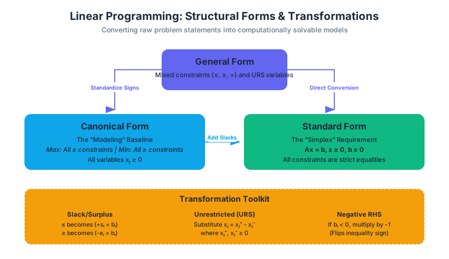
Linear Programming (LP) is the cornerstone of modern operations research, providing a rigorous framework for optimizing a linear objective function subject to linear equality and inequality constraints. While real-world problems—ranging from supply chain logistics to portfolio optimization—naturally manifest in "General Form," the algorithms we use to solve them, such as the Simplex Method or Interior Point Methods, require highly specific mathematical structures.
This article explores the formal definitions of Standard and Canonical forms, the linear algebraic foundations required to manipulate them, and the systematic transformation techniques used to bridge the gap between a raw problem statement and a computationally solvable model.
The Mathematical Landscape of Linear Programming
At its core, a Linear Programming Problem (LPP) seeks to find a vector $x \in \mathbb{R}^n$ that maximizes or minimizes a linear function, given a set of linear constraints. However, "linear" is a broad term. Constraints can be "less than or equal to" ($\le$), "greater than or equal to" ($\ge$), or strict equalities ($=$). Variables can be non-negative, non-positive, or unrestricted in sign (URS).
To manage this variety, mathematicians established two primary templates. Mastery of these forms is not merely an academic exercise; it is a prerequisite for understanding Duality Theory and the mechanics of the Simplex Tableau.
The General Form
A General LPP is expressed as: $$\text{Optimize } z = \sum_{j=1}^{n} c_j x_j$$ Subject to: $$\sum_{j=1}^{n} a_{ij} x_j \quad {\le, =, \ge} \quad b_i \quad \text{for } i = 1, \dots, m$$ $$x_j \text{ is } {\ge 0, \le 0, \text{ or unrestricted}}$$
Canonical Form: The Inequality Baseline
The Canonical Form is most frequently associated with the initial setup of a maximization problem. It is characterized by a uniform direction of inequalities and strict non-negativity of variables.
Definition: Canonical Form (Maximization) A maximization problem is in canonical form if:
- The objective function is to be maximized.
- All constraints are of the $\le$ type.
- All decision variables are non-negative ($x_j \ge 0$).
Why Canonical Form Matters
Canonical form is the natural language of resource allocation. If $b_i$ represents the total amount of resource $i$ available, and $a_{ij}$ represents the amount of resource $i$ consumed by one unit of activity $j$, the constraint $\sum a_{ij} x_j \le b_i$ logically represents the physical reality that you cannot consume more than you possess.
| Feature | Maximization Canonical | Minimization Canonical |
|---|---|---|
| Objective | Maximize $z$ | Minimize $w$ |
| Constraint Type | All $\le$ | All $\ge$ |
| Right-Hand Side ($b_i$) | Unrestricted (usually $\ge 0$) | Unrestricted (usually $\ge 0$) |
| Variables | All $x_j \ge 0$ | All $x_j \ge 0$ |
Standard Form: The Equality Baseline
While Canonical form is intuitive for modeling, Standard Form is the requirement for the Simplex algorithm. Simplex operates by moving along the edges of a polytope, and these edges are mathematically easier to track when constraints are expressed as a system of linear equations ($Ax = b$) rather than inequalities.
Definition: Standard Form An LPP is in Standard Form if:
- The objective function can be either Maximize or Minimize (though many textbooks default to Minimize).
- All constraints are expressed as equalities ($=$).
- All right-hand side constants are non-negative ($b_i \ge 0$).
- All variables are non-negative ($x_j \ge 0$).
The Anatomy of Standard Form
In matrix notation, the Standard Form is written as: $$\min c^T x$$ $$\text{subject to } Ax = b$$ $$x \ge 0, b \ge 0$$ Where $A$ is an $m \times n$ matrix of coefficients, $x$ is the $n \times 1$ vector of variables, and $b$ is the $m \times 1$ vector of requirements.
Transformation Techniques: From General to Standard
Converting a problem into Standard Form involves a series of "moves" that preserve the feasible region's logic while altering its algebraic expression.
1. Converting Inequalities (Slack and Surplus Variables)
To turn an inequality into an equality, we introduce an auxiliary variable.
- Slack Variables ($s_i$): Added to $\le$ constraints. It represents the "unused" portion of a resource.
- Example: $2x_1 + 3x_2 \le 10 \implies 2x_1 + 3x_2 + s_1 = 10, s_1 \ge 0$.
- Surplus Variables ($e_i$): Subtracted from $\ge$ constraints. It represents the "excess" over a minimum requirement.
- Example: $5x_1 + x_2 \ge 8 \implies 5x_1 + x_2 - e_1 = 8, e_1 \ge 0$.
2. Handling Unrestricted Variables (URS)
If a variable $x_j$ can be any real number, we decompose it into the difference of two non-negative variables: $$x_j = x_j^+ - x_j^- \quad \text{where } x_j^+, x_j^- \ge 0$$ Every instance of $x_j$ in the objective function and constraints is replaced by $(x_j^+ - x_j^-)$.
3. Managing Negative Right-Hand Sides
If $b_i < 0$, the entire constraint must be multiplied by $-1$. Note that this flips the inequality sign before you add slack/surplus variables.
- Example: $-2x_1 + x_2 \le -5 \implies 2x_1 - x_2 \ge 5$.
4. Objective Function Reversal
Minimizing $f(x)$ is mathematically equivalent to maximizing $-f(x)$. $$\min z = \sum c_j x_j \iff \max -z = \sum -c_j x_j$$
| Problem Element | Transformation Action | Resulting Form |
|---|---|---|
| Constraint $\le$ | Add Slack Variable ($+s_i$) | Equality ($=$) |
| Constraint $\ge$ | Subtract Surplus Variable ($-e_i$) | Equality ($=$) |
| Variable $x_j \le 0$ | Substitute $x_j = -x_j'$ | $x_j' \ge 0$ |
| Variable $x_j$ URS | Substitute $x_j = x_j^+ - x_j^-$ | $x_j^+, x_j^- \ge 0$ |
| RHS $b_i < 0$ | Multiply constraint by $-1$ | $b_i > 0$ |
Linear Algebra Review: Gauss-Jordan and Bases
Standard form $Ax = b$ is essentially a system of linear equations. However, in LP, we usually have more variables than constraints ($n > m$). This means there are infinitely many solutions. We are interested in Basic Feasible Solutions (BFS).
The Gauss-Jordan Method
In Chapter 0 of the curriculum, the Gauss-Jordan method is highlighted as a tool to transform the matrix $A$ into Reduced Row Echelon Form (RREF). In the context of LP, we use a variation of this to identify a Basis.
A Basis $B$ is a set of $m$ linearly independent columns from $A$. If we set the $n-m$ variables not in the basis (non-basic variables) to zero, we can solve for the $m$ basic variables. If the resulting values are $\ge 0$, we have found a BFS.
The Fundamental Theorem of Linear Programming If an optimal solution to an LPP exists, there exists a Basic Feasible Solution that is optimal.
This theorem is why we convert to Standard Form: it allows us to use row operations to jump from one BFS to another (which is exactly what the Simplex method does).
Implementation: Converting LPPs Programmatically
In modern engineering, we rarely perform these conversions by hand. However, understanding the underlying logic is critical for debugging model infeasibility.
1. Low-Level Implementation (Python/NumPy)
The following snippet demonstrates how to programmatically add slack variables to a constraint matrix.
import numpy as np

def convert_to_standard_form(A, b, constraint_types):
    """
    Adds slack and surplus variables to matrix A.
    constraint_types: list of strings ('<=', '>=', '=')
    """
    m, n = A.shape
    new_cols = []

    for i, t in enumerate(constraint_types):
        col = np.zeros(m)
        if t == '<=':
            col[i] = 1  # Add slack
            new_cols.append(col)
        elif t == '>=':
            col[i] = -1 # Subtract surplus
            new_cols.append(col)
        # '=' requires no additional variable here

    A_standard = np.hstack([A] + [c.reshape(-1, 1) for c in new_cols])
    return A_standard

# Example Usage:
# 2x1 + 3x2 <= 10
# 1x1 + 5x2 >= 5
A = np.array([[2, 3], [1, 5]], dtype=float)
b = np.array([10, 5])
types = ['<=', '>=']

A_std = convert_to_standard_form(A, b, types)
print("Standard Form Matrix A:\n", A_std)
2. Mathematical Derivation (Pseudocode/LaTeX)
The logic for handling unrestricted variables (URS) is often handled at the pre-processing stage of a solver.
ALGORITHM: Handle_URS_Variables
INPUT: Matrix A, Objective c, Variable_Bounds bounds
OUTPUT: Modified A', c', bounds'

FOR EACH variable x_j in Problem:
    IF bounds[j] is (-infinity, +infinity):
        1. Create two new variables: x_j_pos, x_j_neg
        2. Set bounds[x_j_pos] = [0, +infinity]
        3. Set bounds[x_j_neg] = [0, +infinity]
        4. Replace column A[:, j] with two columns: [A[:, j], -A[:, j]]
        5. Replace c[j] in objective with [c[j], -c[j]]
        6. Remove original x_j
    ELSE IF bounds[j] is (-infinity, 0]:
        1. Substitute x_j = -x_j_new
        2. Set bounds[x_j_new] = [0, +infinity]
        3. Multiply column A[:, j] by -1
        4. Multiply c[j] by -1
3. Real-World Usage (CLI/Config)
Many high-level solvers (like Gurobi or CPLEX) allow you to define problems in a natural format, but they provide logs showing the "presolve" conversion to standard form.
# Example: production_plan.lp (LP File Format)
Maximize
  obj: 5 x1 + 4 x2
Subject To
  labor: 2 x1 + 1 x2 <= 20
  materials: 3 x1 + 3 x2 <= 30
Bounds
  x1 >= 0
  x2 >= 0
End
To see how a solver views this, one might use a CLI tool to convert it to a .mps (Mathematical Programming System) file, which is the industry standard for representing LPPs in a structured, matrix-like format.
# Using a tool like 'glpsol' (GLPK) to check problem stats
glpsol --lp production_plan.lp --check --wmps production_plan.mps

# The resulting MPS file will explicitly list rows (constraints)
# and columns (variables), effectively showing the Standard Form
# structure used by the underlying solver engine.
Common Pitfalls and Edge Cases
- Ignoring the RHS Sign: A common mistake is adding a slack variable to a $\le$ constraint where the RHS is negative (e.g., $x_1 \le -5$). You must first multiply by $-1$ to get $-x_1 \ge 5$, then subtract a surplus variable. Failure to do this results in an initial basic solution that is infeasible ($s_1 = -5$).
- Redundant Constraints: In Standard Form, we assume the rows of $A$ are linearly independent. If they are not (e.g., one constraint is just a multiple of another), the Gauss-Jordan elimination will produce a row of zeros. This must be handled to avoid singular matrices during the Simplex process.
- The "URS" Explosion: Replacing every URS variable with two non-negative variables doubles the number of columns for those variables. In large-scale industrial problems, this can significantly increase memory usage. Modern solvers often use "Range Constraints" or specialized URS handling to mitigate this.
- Strict Inequalities: Linear Programming does not handle strict inequalities ($<$ or $>$). The feasible region must be a closed set (a polytope) to guarantee that a maximum or minimum can be reached on the boundary. If a problem has $x < 10$, it is typically modeled as $x \le 10 - \epsilon$, though this is rarely ideal.
Summary of Transformation Workflow
To take any LPP and prepare it for the Simplex Method:
- Standardize the Objective: Convert to Minimize (or Maximize, depending on your algorithm's convention).
- Ensure $b \ge 0$: Multiply any constraint with a negative RHS by $-1$.
- Convert to Equalities: Add slack variables to $\le$ and subtract surplus variables from $\ge$.
- Enforce Non-negativity: Replace URS variables with $x^+ - x^-$ and negative variables with their negated counterparts.
- Verify Linear Independence: Use Gauss-Jordan (Chapter 0 techniques) to ensure the constraint matrix $A$ has full row rank.
Graphical Optimization and the Geometric Method
Key concepts: Feasible Region · Extreme Point Theorem · Level Curves · Vertices · Boundedness
Solving 2D linear programming problems using geometric visualization, feasible regions, and level curves.
Graphical Optimization and the Geometric Method
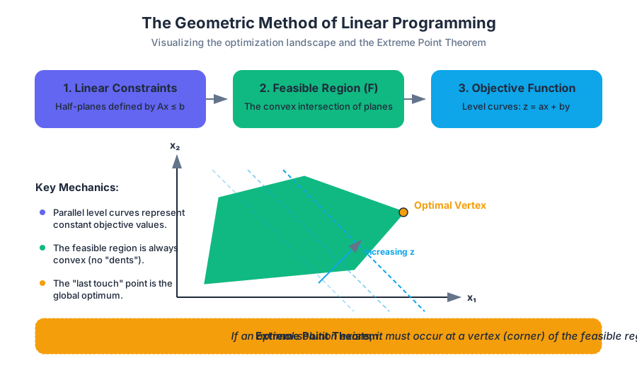
In the study of Linear Programming (LP), the Geometric Method serves as the foundational bridge between abstract algebraic constraints and spatial intuition. While modern industrial solvers handle problems with millions of variables using the Simplex method or Interior Point methods, the core logic of these algorithms is rooted in the geometry of two and three dimensions.
For problems involving only two decision variables, we can visualize the entire optimization landscape. This visualization reveals the "why" behind the "how"—explaining why optimal solutions naturally gravitate toward the "corners" of the search space and how the objective function "scans" the feasible region to find the best possible outcome.
The Anatomy of a Linear Program
Before applying geometric techniques, we must understand the structure of the problem. A linear program consists of an objective function to be maximized or minimized, subject to a set of linear constraints and non-negativity requirements.
Standard vs. Canonical Form
In mathematical optimization, the representation of the problem dictates the method of solution.
- Standard Form: Typically characterized by a maximization objective, all constraints expressed as "less-than-or-equal-to" ($\le$) inequalities, and all variables restricted to non-negative values.
- Canonical Form: Characterized by equality constraints ($Ax = b$), achieved by introducing slack variables to "soak up" the difference between the left and right sides of an inequality.
| Feature | Standard Form | Canonical Form |
|---|---|---|
| Objective | Maximize $z = \mathbf{c}^T\mathbf{x}$ | Maximize $z = \mathbf{c}^T\mathbf{x}$ |
| Constraints | $A\mathbf{x} \le \mathbf{b}$ | $A\mathbf{x} = \mathbf{b}$ |
| Variables | $\mathbf{x} \ge 0$ | $\mathbf{x} \ge 0$ (including slacks) |
| Geometric View | Intersection of half-planes | Intersection of hyperplanes and orthants |
| Primary Use | Graphical Method / Initial Setup | Simplex Method / Matrix Algebra |
The Feasible Region: Geometry of Constraints
The Feasible Region (often denoted as $\mathcal{F}$) is the set of all points $(x, y)$ that satisfy every constraint in the system simultaneously.
Mathematical Definition
Mathematically, each linear inequality of the form $ax + by \le c$ defines a half-plane in $\mathbb{R}^2$. The feasible region is the intersection of these half-planes.
Definition: Convexity A set $\mathcal{F}$ is convex if, for any two points $P_1, P_2 \in \mathcal{F}$, the entire line segment connecting $P_1$ and $P_2$ also lies within $\mathcal{F}$.
In Linear Programming, the feasible region is always a convex polytope (a polygon in 2D, a polyhedron in 3D). This property is critical because it ensures that there are no "local" optima that are not also "global" optima. If you find a peak in a convex region, it is the only peak.
Constructing the Region
- Treat inequalities as equations: Graph the lines $ax + by = c$.
- Identify the valid side: Use a test point (usually $(0,0)$) to determine which side of the line satisfies the inequality.
- Find the intersection: The region where all shaded areas overlap is the feasible region.
- Apply non-negativity: Restrict the region to the first quadrant ($x \ge 0, y \ge 0$).
Level Curves and the Objective Function
The objective function $z = f(x, y) = ax + by$ defines a surface in three-dimensional space. However, in the geometric method, we project this onto the 2D plane using Level Curves (also known as isoclines or objective lines).
Mechanics of Level Curves
A level curve represents all points $(x, y)$ that yield the same value for $z$. For example, if $z = 2x + 3y$, the level curve for $z=6$ is the line $2x + 3y = 6$.
As we change the value of $z$, the level curve shifts across the plane. Crucially, all level curves for a linear objective function are parallel to each other. Their slope is determined by the ratio of the coefficients of the decision variables: $m = -a/b$.
The Optimization "Scan"
To solve the problem graphically:
- Draw a "base" level curve for an arbitrary value of $z$ (e.g., $z=0$).
- Move this line in the direction of increasing $z$ (for maximization) or decreasing $z$ (for minimization).
- The last point in the feasible region that the level curve touches before exiting the region is the optimal solution.
The Extreme Point Theorem
Why do we only look at the corners? This is answered by the Extreme Point Theorem (or the Fundamental Theorem of Linear Programming).
Theorem: Extreme Point Theorem If a linear programming problem has an optimal solution, then at least one optimal solution occurs at an extreme point (vertex) of the feasible region.
Derivation and Logic
Consider the feasible region $\mathcal{F}$. If the optimal solution were in the interior of $\mathcal{F}$, we could move a small distance in the direction of the objective function's gradient to increase $z$, meaning the interior point could not have been optimal. Therefore, the optimum must lie on the boundary.
If the optimum lies on a boundary line segment but not at a vertex, then every point on that segment yields the same $z$ value. This implies that the vertices at the ends of that segment are also optimal. Thus, we are mathematically justified in only checking the vertices.
| Element | Geometric Description | Algebraic Description |
|---|---|---|
| Vertex | A "corner" where two or more boundary lines intersect. | A Basic Feasible Solution (BFS). |
| Edge | A line segment connecting two adjacent vertices. | A path where one constraint is tight and others vary. |
| Interior | Points not on any constraint boundary. | Solutions where all slack variables are non-zero. |
Worked Example: Maximization with Multiple Constraints
Consider the following problem from Participation #2: Maximize $z = 2x + 3y$ Subject to:
- $x + 3y \le 9$
- $2x + 3y \le 12$
- $x \ge 0, y \ge 0$
Step 1: Find the Vertices
We find the vertices by solving the systems of equations formed by the intersection of the boundary lines.
- Origin: $(0, 0)$
- Y-intercept of (1): Set $x=0$ in $x + 3y = 9 \implies y=3$. Point: $(0, 3)$.
- X-intercept of (2): Set $y=0$ in $2x + 3y = 12 \implies x=6$. Point: $(6, 0)$.
- Intersection of (1) and (2): Subtract (1) from (2): $(2x + 3y) - (x + 3y) = 12 - 9 \implies x = 3$. Substitute $x=3$ into (1): $3 + 3y = 9 \implies 3y = 6 \implies y = 2$. Point: $(3, 2)$.
Step 2: Evaluate the Objective Function
We test each vertex in the objective function $z = 2x + 3y$.
| Vertex $(x, y)$ | $z = 2x + 3y$ | Status |
|---|---|---|
| $(0, 0)$ | $2(0) + 3(0) = 0$ | Minimum |
| $(0, 3)$ | $2(0) + 3(3) = 9$ | |
| $(6, 0)$ | $2(6) + 3(0) = 12$ | |
| $(3, 2)$ | $2(3) + 3(2) = 12$ | Optimal (Tie) |
Note: In this specific case, both $(6,0)$ and $(3,2)$ yield $z=12$. This indicates that the objective function line is parallel to the constraint line $2x + 3y = 12$. Every point on the segment connecting these two vertices is optimal.
Implementation: Computational Geometry
While we visualize in 2D, we often use libraries to solve these problems. Below is a Python implementation using SciPy to solve the example above, followed by a low-level conceptual look at how we might verify a vertex's feasibility in C.
import numpy as np
from scipy.optimize import linprog

# Objective: Maximize z = 2x + 3y
# Note: linprog only minimizes, so we minimize -z = -2x - 3y
c = [-2, -3]

# Inequality constraints matrix A_ub * x <= b_ub
# x + 3y <= 9
# 2x + 3y <= 12
A = [[1, 3],
     [2, 3]]
b = [9, 12]

# Bounds for x and y (non-negativity)
x_bounds = (0, None)
y_bounds = (0, None)

res = linprog(c, A_ub=A, b_ub=b, bounds=[x_bounds, y_bounds], method='highs')

print(f"Optimal Value: {-res.fun}")
print(f"Coordinates: x={res.x[0]}, y={res.x[1]}")
The mathematical transformation from an inequality to a canonical equality (Participation #3) is the precursor to the Simplex algorithm.
\begin{aligned}
&\text{Maximize } z = 4x_1 + 2x_2 + 7x_3 \\
&\text{Subject to:} \\
&2x_1 - x_2 + 4x_3 + s_1 = 18 \\
&4x_1 + 2x_2 + 5x_3 + s_2 = 10 \\
&x_1, x_2, x_3, s_1, s_2 \ge 0
\end{aligned}
In a systems-level context, checking if a point is a "vertex" involves verifying linear independence of the active constraints.
#include <stdio.h>
#include <stdbool.h>

/**
 * Simple check to see if a point (x, y) violates any constraints.
 * In a real engine, this would use an epsilon for floating point comparison.
 */
bool is_feasible(float x, float y, float A[2][2], float b[2]) {
    if (x < 0 || y < 0) return false;

    for (int i = 0; i < 2; i++) {
        if ((A[i][0] * x + A[i][1] * y) > b[i] + 0.0001f) {
            return false;
        }
    }
    return true;
}

int main() {
    float A[2][2] = {{1, 3}, {2, 3}};
    float b[2] = {9, 12};

    float test_x = 3.0, test_y = 2.0;

    if (is_feasible(test_x, test_y, A, b)) {
        printf("Point (%.2f, %.2f) is feasible.\n", test_x, test_y);
    } else {
        printf("Point (%.2f, %.2f) violates constraints.\n", test_x, test_y);
    }

    return 0;
}
Boundedness and Special Cases
Not every linear program results in a neat, single-point solution. The geometry of the problem can lead to four distinct outcomes.
| Outcome | Geometric Description | Practical Meaning |
|---|---|---|
| Unique Optimal | The level curve hits exactly one vertex last. | One clear best strategy. |
| Alternative Optima | The level curve is parallel to a constraint edge. | Multiple strategies yield the same best result. |
| Unbounded | The feasible region is "open" in the direction of improvement. | The model is missing a constraint; profit is infinite. |
| Infeasible | The constraints do not overlap; no feasible region exists. | The requirements are contradictory (e.g., $x \le 2$ and $x \ge 5$). |
Unboundedness
An unbounded solution occurs when the feasible region extends infinitely in a direction that allows the objective function to increase (or decrease) without limit. In the real world, this usually indicates a flawed model—no physical system allows for infinite profit or zero cost with infinite production.
Infeasibility
Infeasibility is often encountered in complex projects where resources are over-constrained. Geometrically, this means the intersection of the half-planes is the empty set.
From 2D Geometry to N-Dimensional Algebra
The Graphical Method is limited to 2 or 3 variables because humans cannot visualize higher-dimensional polytopes (hyper-polyhedra). However, the logic holds:
- In $N$ dimensions, a constraint is a hyperplane.
- The feasible region is a convex simplex.
- The optimal solution is still at a vertex.
The Simplex Method is essentially an algebraic "walk" along the edges of this high-dimensional shape. It starts at one vertex (usually the origin) and moves to an adjacent vertex that improves the objective function value, continuing until no further improvement is possible.
Basic Feasible Solutions (BFS) and Slack Variables
Key concepts: Slack Variables · Basic Variables · Non-basic Variables · Basic Feasible Solution (BFS) · Linearly Independent Columns
Bridging the gap between geometry and algebra by identifying vertices through matrix subsets.
Basic Feasible Solutions (BFS) and Slack Variables
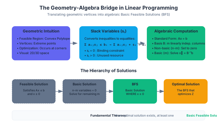
In the domain of Linear Programming (LP), the transition from geometric intuition to algebraic computation is the "Great Leap Forward" that allows us to solve problems with thousands of variables. While we can visualize a feasible region in two or three dimensions as a convex polyhedron, human intuition fails in higher dimensions. To solve these problems algorithmically—specifically via the Simplex Method—we must translate the geometric concept of "vertices" or "corners" into the algebraic language of Basic Feasible Solutions (BFS).
This article explores the mechanics of this translation, the role of Slack Variables in standardizing constraints, and the rigorous linear algebra required to identify the optimal points of a system.
The Geometry-Algebra Bridge
At its core, a Linear Programming Problem (LPP) seeks to optimize a linear objective function subject to linear constraints. Geometrically, the set of all points satisfying these constraints forms a Feasible Region (a convex polytope). The Fundamental Theorem of Linear Programming states that if an optimal solution exists, at least one extreme point (vertex) of the feasible region must be optimal.
To find these vertices algebraically, we use the concept of a BFS. A BFS is essentially the algebraic representation of a vertex.
The Hierarchy of Solutions
| Term | Definition | Geometric Equivalent |
|---|---|---|
| Feasible Solution | Any point $x$ that satisfies all constraints $Ax \le b$ and $x \ge 0$. | Any point inside or on the boundary of the polyhedron. |
| Basic Solution | A solution where $n-m$ variables are set to zero, and the remaining $m$ variables are solved via $Ax = b$. | An intersection point of $n$ constraint hyperplanes. |
| Basic Feasible Solution (BFS) | A Basic Solution that also satisfies the non-negativity constraints ($x \ge 0$). | A vertex (extreme point) of the feasible region. |
| Optimal Solution | A BFS that maximizes or minimizes the objective function. | The "best" vertex. |
Slack Variables: Standardizing the System
Most real-world constraints are inequalities (e.g., "Total labor hours must be less than or equal to 40"). However, linear algebra is built for systems of equations ($Ax = b$). To bridge this gap, we introduce Slack Variables.
Definition and Motivation
A slack variable $s_i$ represents the difference between the left-hand side and the right-hand side of a $\le$ constraint. It quantifies the "unused" portion of a resource.
Definition: Slack Variable For a constraint of the form $\sum a_{ij}x_j \le b_i$, we define a non-negative variable $s_i \ge 0$ such that: $$\sum a_{ij}x_j + s_i = b_i$$ If $s_i = 0$, the constraint is binding (the resource is fully consumed). If $s_i > 0$, the constraint is non-binding.
Transforming to Standard Form
To perform algebraic operations, we must convert the LPP into Standard Form. This requires:
- All constraints are expressed as equalities (using slack or surplus variables).
- All variables are non-negative ($x_i \ge 0$).
- The right-hand side constants are non-negative ($b_i \ge 0$).
Example: Converting to Standard Form
Consider the following non-standard model: Maximize $z = 3x_1 + 2x_2$ Subject to: $2x_1 + x_2 \le 4$ $x_1 + 2x_2 \le 5$ $x_1, x_2 \ge 0$
By adding slack variables $s_1$ and $s_2$, we get the standard form: $2x_1 + x_2 + s_1 = 4$ $x_1 + 2x_2 + s_2 = 5$ $x_1, x_2, s_1, s_2 \ge 0$
Basic and Non-basic Variables
Once in standard form, we have a system of $m$ linear equations with $n$ variables (where $n > m$). This system is underdetermined, meaning it has infinitely many solutions. To find the "corners," we restrict our search.
The $n-m$ Rule
To find a Basic Solution:
- Choose $n-m$ variables and set them to zero. These are called Non-basic Variables (NBV).
- Solve the remaining $m$ equations for the $m$ remaining variables. These are called Basic Variables (BV).
- The set of columns in matrix $A$ corresponding to the basic variables must be Linearly Independent. This set of columns forms a Basis $B$.
Mathematical Representation
Let $A$ be an $m \times n$ matrix of rank $m$. We can partition $A$ into $[B | N]$, where $B$ is an $m \times m$ invertible matrix (the basis) and $N$ is the remaining $m \times (n-m)$ matrix. The equation $Ax = b$ becomes: $$Bx_B + Nx_N = b$$ Setting $x_N = 0$ (Non-basic variables), we solve for $x_B$: $$x_B = B^{-1}b$$
Linear Independence: The Foundation of a Basis
A set of variables can only be "Basic" if their corresponding columns in the constraint matrix $A$ are linearly independent. If the columns are dependent, the matrix $B$ is singular (not invertible), and we cannot solve for a unique $x_B$.
Identifying Linear Independence
As seen in advanced linear algebra (and referenced in Homework 1, Section 0.6), a set of vectors $S = {v_1, v_2, \dots, v_k}$ is linearly independent if the only solution to $c_1v_1 + c_2v_2 + \dots + c_kv_k = 0$ is $c_1 = c_2 = \dots = c_k = 0$.
In the context of BFS, if we pick $m$ columns that are linearly dependent, those variables cannot form a basis. This usually happens when constraints are redundant.
Comparison of Variable States
| State | Variable Type | Value | Interpretation |
|---|---|---|---|
| Non-basic | $x_N$ | Always $0$ | The variable is "at its bound." |
| Basic (Feasible) | $x_B$ | $\ge 0$ | The variable is part of the current solution. |
| Basic (Infeasible) | $x_B$ | $< 0$ | Algebraically valid, but physically impossible (violates $x \ge 0$). |
Implementation: Finding All BFS
While the Simplex method intelligently moves between BFS, a brute-force approach to understanding the concept involves calculating all possible basic solutions and filtering for feasibility.
Python Implementation (NumPy)
This script demonstrates how to extract a basis and solve for basic variables using matrix inversion.
import numpy as np
from itertools import combinations

def find_all_bfs(A, b):
    """
    Finds all Basic Feasible Solutions for a system Ax = b, x >= 0.
    A: m x n matrix
    b: m x 1 vector
    """
    m, n = A.shape
    bfs_list = []

    # Iterate through all possible combinations of m columns
    for indices in combinations(range(n), m):
        B = A[:, indices]

        # Check if the columns are linearly independent (Basis is invertible)
        if np.linalg.matrix_rank(B) == m:
            # Solve B * x_B = b -> x_B = B^-1 * b
            x_b = np.linalg.solve(B, b)

            # Check for feasibility (all components >= 0)
            if np.all(x_b >= -1e-9):  # Using a small epsilon for float precision
                full_solution = np.zeros(n)
                for i, val in enumerate(indices):
                    full_solution[val] = x_b[i]
                bfs_list.append(full_solution)

    return np.unique(bfs_list, axis=0)

# Example: 2x1 + x2 + s1 = 4; x1 + 2x2 + s2 = 5
A_mat = np.array([[2, 1, 1, 0],
                  [1, 2, 0, 1]])
b_vec = np.array([4, 5])

solutions = find_all_bfs(A_mat, b_vec)
print("Basic Feasible Solutions:")
for sol in solutions:
    print(sol)
Mathematical Derivation (LaTeX)
The following block outlines the formal derivation of a Basic Solution.
\text{Given } Ax = b, \text{ partition } x \text{ into } (x_B, x_N):
\begin{pmatrix} B & N \end{pmatrix} \begin{pmatrix} x_B \\ x_N \end{pmatrix} = b

\text{Expand the matrix multiplication:}
B x_B + N x_N = b

\text{Set non-basic variables to zero: } x_N = \mathbf{0}
B x_B + N(\mathbf{0}) = b
B x_B = b

\text{If } B \text{ is non-singular (linearly independent columns):}
x_B = B^{-1}b

\text{The full basic solution is: } x = \begin{pmatrix} B^{-1}b \\ 0 \end{pmatrix}
\text{The solution is Feasible if: } B^{-1}b \ge 0
Worked Example: The "Corner" Hunt
Let's solve for the BFS of the following system:
- $x_1 + x_2 + s_1 = 4$
- $2x_1 + x_2 + s_2 = 6$ $x_1, x_2, s_1, s_2 \ge 0$
Here, $n=4$ (variables) and $m=2$ (constraints). We must set $n-m = 2$ variables to zero.
Case 1: Set $x_1, x_2 = 0$ (Non-basic)
- Basic variables: $s_1, s_2$
- Equations: $s_1 = 4, s_2 = 6$
- Solution: $(0, 0, 4, 6)$. All $\ge 0$, so this is a BFS. (Geometric origin).
Case 2: Set $s_1, s_2 = 0$ (Non-basic)
- Basic variables: $x_1, x_2$
- Equations:
- $x_1 + x_2 = 4$
- $2x_1 + x_2 = 6$
- Subtracting (1) from (2): $x_1 = 2$. Substituting back: $x_2 = 2$.
- Solution: $(2, 2, 0, 0)$. All $\ge 0$, so this is a BFS.
Case 3: Set $x_1, s_1 = 0$ (Non-basic)
- Basic variables: $x_2, s_2$
- Equations:
- $x_2 = 4$
- $x_2 + s_2 = 6 \implies 4 + s_2 = 6 \implies s_2 = 2$
- Solution: $(0, 4, 0, 2)$. All $\ge 0$, so this is a BFS.
Summary of Solutions for this Example
| Combination (NBV) | Basic Variables | Solution $(x_1, x_2, s_1, s_2)$ | Feasible? |
|---|---|---|---|
| ${x_1, x_2}$ | ${s_1, s_2}$ | $(0, 0, 4, 6)$ | Yes |
| ${s_1, s_2}$ | ${x_1, x_2}$ | $(2, 2, 0, 0)$ | Yes |
| ${x_1, s_1}$ | ${x_2, s_2}$ | $(0, 4, 0, 2)$ | Yes |
| ${x_2, s_2}$ | ${x_1, s_1}$ | $(3, 0, 1, 0)$ | Yes |
| ${x_2, s_1}$ | ${x_1, s_2}$ | $(4, 0, 0, -2)$ | No (Infeasible) |
Common Pitfalls and Mastery Checks
When calculating BFS, several technical hurdles can lead to errors. Referring to the Mastery Rubric, a "Mastery+" level understanding requires recognizing these edge cases.
1. Degeneracy
A BFS is degenerate if one or more basic variables equal zero. Geometrically, this means more than $n$ hyperplanes intersect at a single point. This can cause the Simplex method to "cycle" (loop infinitely) unless specific anti-cycling rules (like Bland's Rule) are applied.
2. Linear Dependence
Choosing $m$ columns that are not linearly independent. Error: Attempting to invert a singular matrix. Solution: Ensure the chosen basis $B$ has a non-zero determinant.
3. Infeasibility
Finding a basic solution where $x_i < 0$. Error: Thinking every intersection of lines is a BFS. Reality: Only intersections within the first quadrant (or orthant) are feasible.
4. Standard Form Errors
Forgetting to transform $\ge$ constraints correctly. Correction: For $Ax \ge b$, we subtract a Surplus Variable and add an Artificial Variable to find an initial BFS.
Real-World Usage: Production Libraries
In production environments, we rarely calculate BFS manually. We use highly optimized solvers like Gurobi, CPLEX, or SciPy's linprog. These libraries use the Revised Simplex Method, which maintains the basis $B$ and its inverse efficiently.
Using SciPy for BFS-based Optimization
from scipy.optimize import linprog

# Objective: Maximize 3x1 + 2x2 -> Minimize -3x1 - 2x2
c = [-3, -2]
A = [[2, 1], [1, 2]]
b = [4, 5]
x0_bounds = (0, None)
x1_bounds = (0, None)

res = linprog(c, A_ub=A, b_ub=b, bounds=[x0_bounds, x1_bounds], method='simplex')

print(f"Optimal Value: {-res.fun}")
print(f"Optimal BFS (x1, x2): {res.x}")
# The slack variables can be found in res.slack
print(f"Slack Variables (s1, s2): {res.slack}")
Self-Reflection: Evaluating Your Understanding
Based on the provided grading rubric, assess your work on BFS problems using the following criteria:
| Mastery Level | Criteria |
|---|---|
| Mastery+ | Correctly identifies all BFS, explains degeneracy if present, and provides clear algebraic derivations for $B^{-1}b$. |
| Mastery | Correctly identifies BFS but may have minor transcription errors in the final vector. |
| Developing | Can convert to standard form and add slack variables but struggles with solving the resulting systems or identifying linear independence. |
| Minimal | Understands that slack variables are needed but cannot solve for basic variables algebraically. |
The Simplex Method and Tableau Optimization
Key concepts: Simplex Tableau · Pivot Selection · Optimality Criterion · Entering and Leaving Variables · Iterative Improvement
The primary algorithmic approach for solving linear programming problems using iterative pivoting.
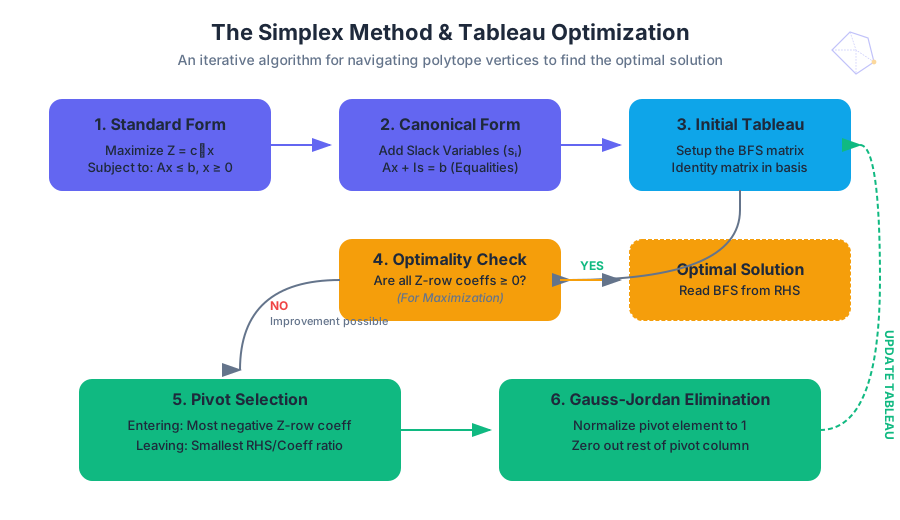
The Simplex Method and Tableau Optimization
The Simplex Method is arguably the most influential algorithm in the history of constrained optimization. Developed by George Dantzig in 1947, it provides a systematic, iterative procedure for navigating the vertices of a high-dimensional polytope to find the optimal value of a linear objective function. While modern interior-point methods offer better theoretical polynomial time complexity, the Simplex algorithm remains the workhorse of industrial solvers due to its efficiency in practice and its unique ability to perform "warm starts" after minor model modifications.
At its core, the Simplex method exploits a fundamental property of Linear Programming (LP): if an optimal solution exists, it must occur at an extreme point (vertex) of the feasible region. Instead of searching the infinite interior of the feasible set, the algorithm "hops" from one vertex to an adjacent one, ensuring that each move improves (or at least maintains) the value of the objective function.
Foundations: Standard and Canonical Forms
Before the Simplex method can be applied, a Linear Programming problem must be expressed in a specific mathematical structure. In academic and professional practice, we distinguish between Standard Form and Canonical Form.
Standard Form
A maximization problem is in Standard Form if:
- The objective function is to be maximized.
- All variables are non-negative ($x_i \ge 0$).
- All constraints are expressed as "less-than-or-equal-to" inequalities ($\sum a_{ij}x_j \le b_i$).
- All right-hand side constants are non-negative ($b_i \ge 0$).
Canonical Form
To perform the algebraic manipulations required by the Simplex method, we must convert inequalities into equalities. This is achieved by introducing Slack Variables. A problem is in Canonical Form if it consists of a system of linear equations $Ax = b$ where a subset of the columns of $A$ forms an identity matrix.
Definition: Slack Variable A non-negative variable $s_i$ added to a $\le$ constraint to convert it into an equality. For example, $2x + 3y \le 6$ becomes $2x + 3y + s_1 = 6$, where $s_1 \ge 0$.
| Feature | Standard Form | Canonical Form |
|---|---|---|
| Constraint Type | Inequalities ($\le$) | Equalities ($=$) |
| Variable Count | Original decision variables | Decision + Slack/Artificial variables |
| Goal | Geometric definition of the polytope | Algebraic setup for Gauss-Jordan elimination |
| RHS ($b$) | Must be non-negative | Must be non-negative |
The Simplex Tableau
The Simplex Tableau is a structured matrix used to organize the coefficients of the objective function and the constraints. It serves as a computational "dashboard" that tracks the current Basic Feasible Solution (BFS).
In any iteration, the variables are partitioned into two sets:
- Basic Variables (BV): Variables that currently form the basis (the identity matrix columns). Their values are determined by the right-hand side.
- Non-Basic Variables (NBV): Variables set to zero.
Tableau Anatomy
A typical maximization tableau is organized as follows:
- The top row (often called the z-row) contains the coefficients of the objective function.
- The remaining rows represent the constraints.
- The last column (RHS) contains the current values of the basic variables.
The Simplex Algorithm: Iterative Improvement
The algorithm follows a rigorous cycle of selection and transformation. Each iteration represents a move from one vertex to an adjacent vertex with a better objective value.
1. Optimality Criterion
We examine the objective row (z-row). In a maximization problem, if all coefficients of the non-basic variables in the z-row are non-negative (assuming the form $z - \sum c_i x_i = 0$), the current solution is optimal. If any coefficients are negative, the objective can still be improved.
2. Pivot Selection: The Entering Variable
The non-basic variable with the most negative coefficient in the z-row is chosen as the Entering Variable. This variable will transition from zero to a positive value in the next iteration. This choice is a heuristic known as "Dantzig's Rule," aimed at increasing the objective function as steeply as possible.
3. The Minimum Ratio Test: The Leaving Variable
To maintain feasibility, we cannot increase the entering variable indefinitely. We must determine which basic variable hits zero first. For every row where the entering variable has a positive coefficient, we calculate the ratio: $$\text{Ratio} = \frac{\text{RHS Value}}{\text{Coefficient of Entering Variable}}$$ The row with the smallest non-negative ratio identifies the Leaving Variable. This row is called the Pivot Row.
4. Pivoting (Gauss-Jordan Elimination)
The intersection of the entering column and the leaving row is the Pivot Element. We perform row operations to:
- Turn the pivot element into a $1$.
- Turn all other elements in the entering column (including the z-row) into $0$.
Implementation: Low-Level Pivot Logic
The following Python implementation using NumPy demonstrates the core mechanics of a single Simplex iteration. Note the use of the minimum ratio test and row-wise transformations.
import numpy as np

def simplex_step(tableau):
    """
    Performs a single pivot iteration on a Simplex Tableau.
    Assumes maximization problem in the form: z - c1x1 - c2x2 ... = 0
    """
    n_rows, n_cols = tableau.shape
    z_row = tableau[0, :-1]

    # 1. Check Optimality / Select Entering Variable (Pivot Column)
    if np.all(z_row >= 0):
        return None, "Optimal"

    pivot_col = np.argmin(z_row)

    # 2. Minimum Ratio Test / Select Leaving Variable (Pivot Row)
    ratios = []
    for i in range(1, n_rows):
        val = tableau[i, pivot_col]
        rhs = tableau[i, -1]
        if val > 0:
            ratios.append(rhs / val)
        else:
            ratios.append(np.inf) # Cannot pivot on non-positive elements

    pivot_row = np.argmin(ratios) + 1 # +1 because we skipped z-row

    if ratios[pivot_row-1] == np.inf:
        return None, "Unbounded"

    # 3. Pivoting
    pivot_val = tableau[pivot_row, pivot_col]
    tableau[pivot_row, :] /= pivot_val

    for r in range(n_rows):
        if r != pivot_row:
            tableau[r, :] -= tableau[r, pivot_col] * tableau[pivot_row, :]

    return tableau, "Iterating"

# Example usage:
# Maximize z = 3x1 + 2x2 subject to 2x1 + x2 <= 4, 2x1 + 3x2 <= 6
# Tableau: [z, x1, x2, s1, s2, RHS]
example_tab = np.array([
    [1, -3, -2, 0, 0, 0],
    [0,  2,  1, 1, 0, 4],
    [0,  2,  3, 0, 1, 6]
], dtype=float)

new_tab, status = simplex_step(example_tab)
print(f"Status: {status}\nUpdated Tableau:\n{new_tab}")
Mathematical Derivation of the Pivot
To understand why the Simplex method works, we must look at the linear algebra of the basis. Let the constraints be $Ax = b$. We partition $A$ into $[B, N]$, where $B$ is the basis matrix (invertible) and $N$ represents non-basic columns.
The solution is given by: $$x_B = B^{-1}b - B^{-1}Nx_N$$ The objective function $z = c^T x$ becomes: $$z = c_B^T(B^{-1}b - B^{-1}Nx_N) + c_N^T x_N$$ $$z = c_B^T B^{-1}b + (c_N^T - c_B^T B^{-1}N)x_N$$
The term $(c_N^T - c_B^T B^{-1}N)$ is known as the Reduced Cost vector. If all reduced costs are non-positive (for maximization), then increasing any $x_N$ (which are currently 0) will decrease $z$. Thus, we are at the optimum.
\begin{aligned}
&\text{Algorithm: Simplex Method}\\
&\text{1: Identify initial BFS by setting } x_{non-basic} = 0 \\
&\text{2: } \mathbf{while} \ \exists \ \bar{c}_j < 0 \ \mathbf{do} \\
&\text{3: } \quad \text{Select } j \text{ such that } \bar{c}_j \text{ is most negative (Entering Variable)} \\
&\text{4: } \quad \mathbf{if} \ A_{ij} \le 0 \ \forall i \ \mathbf{then} \\
&\text{5: } \quad \quad \mathbf{return} \ \text{"Unbounded"} \\
&\text{6: } \quad \text{Select row } i \text{ such that } \frac{b_i}{A_{ij}} = \min_{k: A_{kj}>0} \frac{b_k}{A_{kj}} \text{ (Leaving Variable)} \\
&\text{7: } \quad \text{Perform pivot on } A_{ij} \text{ using Gauss-Jordan elimination} \\
&\text{8: } \mathbf{end \ while} \\
&\text{9: } \mathbf{return} \ \text{Current BFS}
\end{aligned}
Worked Example: Maximizing a Three-Variable System
Consider the following problem from Participation #4: Maximize: $z = 4x_1 + 2x_2 + 7x_3$ Subject to:
- $2x_1 - x_2 + 4x_3 \le 18$
- $4x_1 + 2x_2 + 5x_3 \le 10$
- $x_1, x_2, x_3 \ge 0$
Step 1: Convert to Canonical Form
Introduce slack variables $s_1, s_2$:
- $2x_1 - x_2 + 4x_3 + s_1 = 18$
- $4x_1 + 2x_2 + 5x_3 + s_2 = 10$ Objective: $z - 4x_1 - 2x_2 - 7x_3 = 0$
Step 2: Initial Tableau
| Basis | $z$ | $x_1$ | $x_2$ | $x_3$ | $s_1$ | $s_2$ | RHS |
|---|---|---|---|---|---|---|---|
| $z$ | 1 | -4 | -2 | -7 | 0 | 0 | 0 |
| $s_1$ | 0 | 2 | -1 | 4 | 1 | 0 | 18 |
| $s_2$ | 0 | 4 | 2 | 5 | 0 | 1 | 10 |
Step 3: First Pivot
- Entering: $x_3$ (most negative in z-row: -7).
- Ratios:
- Row 1 ($s_1$): $18 / 4 = 4.5$
- Row 2 ($s_2$): $10 / 5 = 2$
- Leaving: $s_2$ (smallest ratio).
- Pivot Element: 5 (Row 2, Column $x_3$).
After pivoting on 5:
- Divide Row 2 by 5.
- $R_1 \leftarrow R_1 - 4R_2$
- $R_z \leftarrow R_z + 7R_2$
New Tableau:
| Basis | $z$ | $x_1$ | $x_2$ | $x_3$ | $s_1$ | $s_2$ | RHS |
|---|---|---|---|---|---|---|---|
| $z$ | 1 | 1.6 | 0.8 | 0 | 0 | 1.4 | 14 |
| $s_1$ | 0 | -1.2 | -2.6 | 0 | 1 | -0.8 | 10 |
| $x_3$ | 0 | 0.8 | 0.4 | 1 | 0 | 0.2 | 2 |
Result: All coefficients in the z-row are non-negative ($1.6, 0.8, 0, 0, 1.4$). The solution is optimal. Optimal Solution: $x_1=0, x_2=0, x_3=2, z=14$.
Advanced Scenarios and Pitfalls
While the Simplex method is robust, several edge cases can occur during the execution of the algorithm.
1. Degeneracy and Cycling
Degeneracy occurs when one or more basic variables have a value of zero. This happens when there is a tie in the Minimum Ratio Test.
- The Risk: The algorithm might pivot without changing the objective value. In rare cases, it can enter an infinite loop (cycling).
- The Solution: Use Bland’s Rule, which dictates choosing the variable with the lowest index in case of ties.
2. Unboundedness
If the entering variable has no positive coefficients in any constraint row, the ratio test fails.
- Meaning: The feasible region is open in the direction of improvement. The objective function can be increased to infinity.
3. Infeasibility and the Two-Phase Method
If the origin $(0,0,...0)$ is not a feasible solution (e.g., if we have $\ge$ constraints), we cannot start the Simplex method directly.
- Phase I: Introduce Artificial Variables and a new objective function to minimize the sum of these variables. If the minimum is 0, we have found a BFS for the original problem.
- Phase II: Remove artificial variables and solve the original objective.
| Problem State | Tableau Indicator |
|---|---|
| Optimal | All z-row coefficients $\ge 0$ (Max problem). |
| Unbounded | Entering column has all entries $\le 0$. |
| Infeasible | Phase I ends with a non-zero artificial variable. |
| Multiple Optima | A non-basic variable has a 0 coefficient in the optimal z-row. |
Real-World Usage: Large-Scale Solvers
In production environments, we rarely write our own Simplex solvers from scratch. Instead, we use high-performance libraries like Gurobi, CPLEX, or the open-source HiGHS. These solvers use the Revised Simplex Method, which maintains the basis inverse $B^{-1}$ explicitly or via LU factorization to save memory and computation time.
# Example: Solving an LP using the GLPK (GNU Linear Programming Kit)
# 1. Define the problem in a .mod or .lp file
cat <<EOF > problem.lp
Maximize
 obj: 4 x1 + 2 x2 + 7 x3
Subject To
 c1: 2 x1 - 1 x2 + 4 x3 <= 18
 c2: 4 x1 + 2 x2 + 5 x3 <= 10
Bounds
 x1 >= 0
 x2 >= 0
 x3 >= 0
End
EOF

# 2. Run the solver using the Simplex method
glpsol --lp problem.lp -o solution.txt

# 3. View the results
grep "Objective:" solution.txt
Summary of Key Insights
- Geometric Intuition: The Simplex method is a "greedy" walk along the edges of a polytope.
- Algebraic Engine: The tableau is a compact representation of Gauss-Jordan elimination tailored for optimization.
- The Ratio Test: This is the "safety valve" that prevents the algorithm from stepping outside the feasible region.
- Duality: Every Simplex step in the primal problem implicitly provides information about the dual problem (shadow prices), which are represented by the coefficients in the optimal z-row.
By mastering the tableau and the logic of pivots, one gains the ability to not only solve linear programs but to perform sensitivity analysis—understanding how changes in constraints or costs ripple through a complex system.
The Two-Phase Method and Artificial Variables
Key concepts: Artificial Variables · Phase I · Phase II · Infeasibility Detection
Handling problems where an initial basic feasible solution is not immediately obvious.
The Two-Phase Method and Artificial Variables
The Simplex algorithm is the workhorse of linear programming, yet it possesses a fundamental "chicken-and-egg" problem: to begin the optimization process, the algorithm requires an initial Basic Feasible Solution (BFS). For problems where the constraints are all of the "less-than-or-equal-to" ($\le$) variety with non-negative right-hand sides, the origin $(0,0,\dots,0)$ serves as a convenient starting BFS, as the slack variables naturally form an identity matrix in the basis.
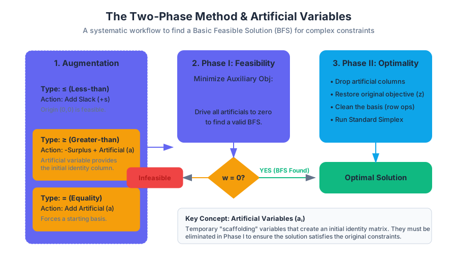
However, real-world engineering and economic models rarely adhere to such convenient geometry. Constraints involving "greater-than-or-equal-to" ($\ge$) or strict equality ($=$) often exclude the origin from the feasible region. In these cases, we cannot simply "start at zero." The Two-Phase Method is the rigorous mathematical framework designed to bridge this gap. It introduces Artificial Variables to create a temporary, synthetic feasible region, finds a valid starting point for the original problem (Phase I), and then proceeds to optimize the true objective (Phase II).
The Challenge of the Initial Basis
In linear programming, a Canonical Form requires a set of basic variables that form an identity matrix within the constraint coefficients. This allows us to read the value of the basic variables directly from the right-hand side ($b$-vector).
When we encounter a constraint like $3x_1 + 2x_2 \ge 10$, we subtract a surplus variable ($s_1$) to convert the inequality to an equation: $3x_1 + 2x_2 - s_1 = 10$. If we set the decision variables $x_1, x_2$ to zero, we are left with $-s_1 = 10$, or $s_1 = -10$. This violates the non-negativity constraint ($s_1 \ge 0$), meaning the origin is not a feasible starting point. Similarly, equality constraints like $x_1 + x_2 = 5$ provide no slack variable to act as a basic variable.
Comparison of Constraint Transformations
| Constraint Type | Transformation Action | Resulting Variable Type | Initial Basis Contribution |
|---|---|---|---|
| Less than ($\le$) | Add Slack ($+s_i$) | Slack Variable | Provides a $+1$ to the Identity Matrix |
| Greater than ($\ge$) | Subtract Surplus ($-s_i$) | Surplus Variable | Provides a $-1$; Cannot be in initial basis |
| Equality ($=$) | None | N/A | No variable provided for basis |
To solve this, we introduce Artificial Variables ($a_i$). These variables have no physical or economic meaning; they exist solely to provide the mathematical "scaffolding" needed to construct an initial identity matrix.
Artificial Variables: The Mathematical Catalyst
An artificial variable is a non-negative variable added to $\ge$ or $=$ constraints to force a starting basis. For the constraint $3x_1 + 2x_2 - s_1 = 10$, we modify it to: $$3x_1 + 2x_2 - s_1 + a_1 = 10$$ Now, by setting $x_1, x_2, s_1$ to zero, we get $a_1 = 10$, which is a valid (though "artificial") BFS.
Definition: Artificial Variable A variable $a_i \ge 0$ added to a linear programming constraint to ensure the existence of a basic feasible solution for the start of the Simplex method. These variables must be driven to zero for the solution to be valid for the original problem.
Phase I: The Search for Feasibility
The goal of Phase I is not to solve the original problem, but to find any feasible solution that satisfies the original constraints. We do this by creating an auxiliary objective function, $w$, which is the sum of all artificial variables.
The Phase I Objective
Minimize: $$w = \sum_{i=1}^{k} a_i$$ Subject to the modified constraints of the original problem.
Why minimize the sum? If the original problem has a feasible region, there must exist a point where all $a_i = 0$. If we minimize $w$ and find that the minimum value is $0$, we have successfully "pushed" the artificial variables out of the basis (or at least reduced them to zero). The resulting values for the original variables ($x_i$) and slack/surplus variables ($s_i$) constitute a BFS for the original problem.
Outcomes of Phase I
| Phase I Result | Interpretation | Action for Phase II |
|---|---|---|
| Min $w = 0$ | A feasible solution to the original problem exists. | Proceed to Phase II using the current BFS. |
| Min $w > 0$ | No feasible solution exists for the original constraints. | Terminate. The problem is Infeasible. |
| Artificials in Basis (at 0) | Degenerate solution; the basis contains an artificial variable at zero. | Perform a special pivot to swap it for a non-artificial variable. |
Phase II: The Search for Optimality
Once Phase I concludes with $w=0$, we discard the artificial variables entirely. We revert to the original objective function ($z$), but we keep the tableau (the basis) reached at the end of Phase I.
The Transition Steps
- Drop Artificial Columns: Remove all columns corresponding to artificial variables from the tableau.
- Restore Original Objective: Replace the $w$ row with the original objective function coefficients.
- Update the Objective Row: Because the current basis might not be "clean" relative to the original objective, we must perform row operations to ensure the coefficients of the basic variables in the $z$-row are zero.
- Simplex Optimization: Run the standard Simplex algorithm until an optimal solution is found or the problem is found to be unbounded.
Implementation: A Python Approach using NumPy
In a production-grade solver, the transition between Phase I and Phase II requires careful handling of floating-point precision to detect if $w$ is truly zero.
import numpy as np

def pivot(tableau, row, col):
    """Performs a Gaussian pivot on the simplex tableau."""
    tableau[row, :] /= tableau[row, col]
    for i in range(len(tableau)):
        if i != row:
            tableau[i, :] -= tableau[i, col] * tableau[row, :]
    return tableau

def solve_phase_i(tableau, num_vars, num_artif):
    """
    Minimizes the sum of artificial variables.
    Tableau structure: [Constraints | RHS]
    The last row is the Phase I objective (w).
    """
    rows, cols = tableau.shape
    # Standard Simplex on Phase I objective
    while np.min(tableau[-1, :-1]) < -1e-9:
        pivot_col = np.argmin(tableau[-1, :-1])

        # Ratio test
        ratios = []
        for i in range(rows - 1):
            if tableau[i, pivot_col] > 1e-9:
                ratios.append(tableau[i, -1] / tableau[i, pivot_col])
            else:
                ratios.append(np.inf)

        pivot_row = np.argmin(ratios)
        if ratios[pivot_row] == np.inf:
            raise Exception("Phase I is unbounded (should not happen with artificials)")

        tableau = pivot(tableau, pivot_row, pivot_col)

    return tableau

# Example usage:
# Minimize w = a1 subject to:
# x1 + x2 + a1 = 5
# x1, x2, a1 >= 0
# Tableau: [x1, x2, a1, RHS]
example_tab = np.array([
    [1.0, 1.0, 1.0, 5.0],
    [-1.0, -1.0, 0.0, -5.0] # w row: -x1 - x2 + 0a1 = -5 (after substitution)
], dtype=float)
Formal Logic and Derivation (LaTeX)
The core of the Two-Phase method is the substitution of the objective function. Before we can start Phase I, we must express the $w$ row in terms of non-basic variables.
\begin{aligned}
&\text{Given a constraint: } \sum a_i = w \\
&\text{And the structural constraints: } A_{original}x + I a = b \\
&\text{We must eliminate } a_i \text{ from the } w \text{ row to start Phase I.} \\
&w = \sum (b_i - \sum A_{ij}x_j) \\
&w + \sum_j (\sum_i A_{ij})x_j = \sum b_i \\
&\text{This gives us the initial coefficients for the Phase I objective row.}
\end{aligned}
Worked Example: Handling Infeasibility
Consider the following problem: Maximize $z = 3x_1 + 2x_2$ Subject to:
- $2x_1 + x_2 \le 2$
- $3x_1 + 4x_2 \ge 12$
- $x_1, x_2 \ge 0$
Step 1: Standard Form with Artificials
- $2x_1 + x_2 + s_1 = 2$
- $3x_1 + 4x_2 - s_2 + a_1 = 12$
- Phase I Objective: Minimize $w = a_1$.
Step 2: Phase I Tableau
We substitute $a_1 = 12 - 3x_1 - 4x_2 + s_2$ into $w$. $w = 12 - 3x_1 - 4x_2 + s_2 \implies w + 3x_1 + 4x_2 - s_2 = 12$.
| Basis | $x_1$ | $x_2$ | $s_1$ | $s_2$ | $a_1$ | RHS |
|---|---|---|---|---|---|---|
| $s_1$ | 2 | 1 | 1 | 0 | 0 | 2 |
| $a_1$ | 3 | 4 | 0 | -1 | 1 | 12 |
| $w$ | -3 | -4 | 0 | 1 | 0 | -12 |
(Note: We use the negative coefficients in the tableau for a minimization problem being treated as a maximization of $-w$).
Step 3: Pivoting
The most negative coefficient in the $w$-row is $-4$ (column $x_2$). Ratio test:
- Row 1: $2/1 = 2$
- Row 2: $12/4 = 3$ Pivot on Row 1, Column $x_2$.
New Tableau:
| Basis | $x_1$ | $x_2$ | $s_1$ | $s_2$ | $a_1$ | RHS |
|---|---|---|---|---|---|---|
| $x_2$ | 2 | 1 | 1 | 0 | 0 | 2 |
| $a_1$ | -5 | 0 | -4 | -1 | 1 | 4 |
| $w$ | 5 | 0 | 4 | 1 | 0 | -4 |
Step 4: Detection
In the $w$-row, all coefficients for non-basic variables ($x_1, s_1, s_2$) are positive. We have reached the minimum for Phase I. However, the RHS for $w$ is $-4$ (meaning $w = 4$). Since $w > 0$, the artificial variable $a_1$ is still in the basis with a value of 4.
Conclusion: The problem is Infeasible. There is no combination of $x_1, x_2$ that satisfies both $2x_1 + x_2 \le 2$ and $3x_1 + 4x_2 \ge 12$.
Common Pitfalls and Troubleshooting
Even experienced engineers stumble on the nuances of the Two-Phase method. The following table highlights common errors, categorized by the mastery rubric of conceptual vs. computational accuracy.
| Error Type | Description | Consequence | Correction |
|---|---|---|---|
| Substitution Failure | Forgetting to eliminate artificial variables from the $w$-row before starting Phase I. | The initial tableau will not be in canonical form; Simplex will fail. | Perform row operations to zero out $a_i$ coefficients in the $w$-row using constraint rows. |
| Surplus Sign Error | Adding a surplus variable instead of subtracting it ($+s_i$ for $\ge$). | The feasible region is mathematically inverted. | Always use $-s_i$ for $\ge$ and $+s_i$ for $\le$. |
| Phase II Transition | Keeping artificial columns in Phase II. | The solver might pivot back into an artificial variable, yielding a non-physical solution. | Delete all $a_i$ columns after Phase I completes with $w=0$. |
| Numerical Instability | Using a strict == 0 check for $w$ in code. |
Floating point errors might make $w = 1e-15$, causing the solver to claim infeasibility. | Use an epsilon tolerance (e.g., if w < 1e-9). |
Real-World Usage: Solver Configuration
In modern optimization suites like Gurobi, CPLEX, or the open-source HiGHS, you rarely write the Two-Phase tableau by hand. Instead, you define the problem in a high-level format. The solver's "Presolve" and "Simplex" engines handle the artificial variables internally.
# Example: Problem definition for a solver-agnostic interface (like Pyomo or PuLP)
problem:
  name: "Production_Optimization"
  sense: maximize
  objective:
    z: "3*x1 + 2*x2"
  constraints:
    - name: "Labor_Limit"
      expression: "2*x1 + x2 <= 4"
    - name: "Minimum_Requirement"
      expression: "3*x1 - 2*x2 >= 6" # This will trigger Phase I / Artificial Variables
  variables:
    x1: { low_bound: 0 }
    x2: { low_bound: 0 }
When you run this through a solver, the logs will often show the Phase I progress:
$ highs_solver model.lp
Presolve: 2 rows, 2 columns, 4 nonzeros
Phase 1: Finding initial feasible solution...
Iter: 0, Obj: 6.000000 (Artificial sum)
Iter: 1, Obj: 0.000000
Phase 1 complete. Feasible solution found.
Phase 2: Optimizing original objective...
Iter: 2, Obj: 9.000000
Optimal solution found.
Advanced Concept: Linear Independence and the Basis
The source material highlights the importance of Linear Independence in vector spaces. In the context of the Two-Phase method, the artificial variables ensure that the set of columns chosen for the basis is linearly independent.
If we have $m$ constraints, we need $m$ linearly independent columns to form a basis. By adding an artificial variable to each "difficult" constraint, we are essentially injecting the standard basis vectors $e_i$ (columns of the identity matrix) into the matrix $A$. Since the standard basis vectors are guaranteed to be linearly independent, we guarantee that a basis exists, allowing the Simplex machinery to start its engine.
Duality in Linear Programming
Key concepts: Primal Problem · Dual Problem · Weak Duality Theorem · Duality Theorem · Shadow Prices
Exploring the relationship between a 'Primal' problem and its 'Dual' counterpart.
Duality in Linear Programming: The Hidden Symmetry of Optimization
In the realm of mathematical optimization, Duality is perhaps the most profound and elegant concept. It suggests that every linear programming (LP) problem, referred to as the Primal, can be viewed from an entirely different perspective, known as the Dual. This is not merely a mathematical curiosity; the relationship between these two problems provides deep insights into the structure of optimization, the value of resources, and the stability of optimal solutions.
As we explore this topic, we will see that the Dual problem is essentially the "mirror image" of the Primal. If the Primal is a maximization of profit subject to resource constraints, the Dual is the minimization of the total value of those resources. This symmetry allows us to solve complex problems more efficiently and perform Sensitivity Analysis—determining how changes in our constraints (like a sudden shortage of raw materials) affect our bottom line.
The Primal and Dual Relationship
To understand duality, we must first establish a standard frame of reference. In linear programming, we often work with the Standard Form or Canonical Form. A Primal problem in maximization form is typically defined by an objective function $z = \mathbf{c}^T\mathbf{x}$, subject to a set of linear inequalities $A\mathbf{x} \le \mathbf{b}$ and non-negativity constraints $\mathbf{x} \ge 0$.
The Dual Problem is constructed using the same parameters ($A, \mathbf{b}, \mathbf{c}$) but rearranged. The coefficients of the Primal objective function become the right-hand side (RHS) of the Dual constraints, and the Primal RHS values become the coefficients of the Dual objective function.
Construction Rules
The transformation from Primal to Dual follows a strict set of mapping rules. These rules ensure that the mathematical integrity of the optimization is preserved across the "mirror."
| Primal Feature (Maximization) | Dual Feature (Minimization) |
|---|---|
| Objective Function $z = \sum c_j x_j$ | Objective Function $w = \sum b_i y_i$ |
| Constraint $i$: $\sum a_{ij} x_j \le b_i$ | Variable $y_i$: $y_i \ge 0$ |
| Constraint $i$: $\sum a_{ij} x_j = b_i$ | Variable $y_i$: $y_i$ is unrestricted (URS) |
| Variable $x_j$: $x_j \ge 0$ | Constraint $j$: $\sum a_{ij} y_i \ge c_j$ |
| Variable $x_j$: $x_j$ is unrestricted (URS) | Constraint $j$: $\sum a_{ij} y_i = c_j$ |
| Constraint Matrix: $A$ | Constraint Matrix: $A^T$ (Transpose) |
Mathematical Derivation
Consider the Primal problem (P): $$\text{Maximize } z = \mathbf{c}^T\mathbf{x}$$ $$\text{subject to } A\mathbf{x} \le \mathbf{b}, \mathbf{x} \ge 0$$
The Dual problem (D) is formulated as: $$\text{Minimize } w = \mathbf{b}^T\mathbf{y}$$ $$\text{subject to } A^T\mathbf{y} \ge \mathbf{c}, \mathbf{y} \ge 0$$
Where:
- $\mathbf{x}$ is a vector of $n$ decision variables.
- $\mathbf{y}$ is a vector of $m$ dual variables (one for each Primal constraint).
- $A$ is an $m \times n$ matrix of coefficients.
Theorem: The Dual of the Dual is the Primal. If you take the Dual of a Dual problem, you will arrive back at the original Primal problem. This confirms the perfectly symmetric nature of the relationship.
The Fundamental Theorems of Duality
The relationship between the Primal and Dual is governed by three critical theorems. These theorems provide the "guarantees" that allow us to use the Dual to solve or verify the Primal.
1. Weak Duality Theorem
The Weak Duality Theorem states that for any feasible solution $\mathbf{x}$ to the Primal and any feasible solution $\mathbf{y}$ to the Dual: $$\mathbf{c}^T\mathbf{x} \le \mathbf{b}^T\mathbf{y}$$
In plain English: any feasible value of the Dual objective function serves as an upper bound for the Primal objective function (in a maximization problem). Conversely, the Primal provides a lower bound for the Dual.
2. Strong Duality Theorem
The Strong Duality Theorem is the cornerstone of LP. It states that if the Primal has an optimal solution $\mathbf{x}^$, then the Dual also has an optimal solution $\mathbf{y}^$, and their objective values are equal: $$z^* = \mathbf{c}^T\mathbf{x}^* = \mathbf{b}^T\mathbf{y}^* = w^*$$
This equality is what allows us to solve the Dual to find the optimal value of the Primal. In many computational scenarios, the Dual might be easier to solve (e.g., if it has fewer constraints than the Primal).
3. Complementary Slackness Theorem
This theorem describes the relationship between the slack variables of one problem and the decision variables of the other. It states that for optimal solutions $\mathbf{x}^$ and $\mathbf{y}^$:
- If a Primal constraint is "slack" (the inequality is not an equality at the optimum), the corresponding Dual variable must be zero.
- If a Primal variable is positive, the corresponding Dual constraint must be "tight" (the inequality holds as an equality).
| Condition | Mathematical Implication |
|---|---|
| $y_i^* > 0$ | $\sum a_{ij} x_j^* = b_i$ (Constraint $i$ is binding) |
| $\sum a_{ij} x_j^* < b_i$ | $y_i^* = 0$ (Resource $i$ is not fully used; its marginal value is zero) |
| $x_j^* > 0$ | $\sum a_{ij} y_i^* = c_j$ (Dual constraint $j$ is binding) |
| $\sum a_{ij} y_i^* > c_j$ | $x_j^* = 0$ (Activity $j$ is too expensive; it is not performed) |
Shadow Prices and Economic Interpretation
One of the most practical applications of duality is the concept of Shadow Prices. In an economic context, if the Primal problem represents maximizing profit from resources, the Dual variables $y_i$ represent the marginal value of those resources.
Definition: Shadow Price The shadow price of a constraint is the amount by which the optimal value of the objective function ($z^*$) would increase if the right-hand side of that constraint ($b_i$) were increased by one unit, assuming the current optimal basis remains the same.
Why Shadow Prices Matter
Imagine a factory that uses labor and electricity to produce goods. If the shadow price of labor is $15, it means that if the factory could acquire one more hour of labor, its total profit would increase by $15. If the market rate for labor is $10/hour, the factory should hire more workers. If the market rate is $20/hour, it should not.
Table: Primal vs. Dual Economic Logic
| Component | Primal Interpretation (Production) | Dual Interpretation (Valuation) |
|---|---|---|
| Variables | Levels of activities (e.g., units to produce) | Unit value of resources (Shadow prices) |
| Objective | Maximize total profit | Minimize total implicit value of resources |
| Constraints | Resource availability limits | Minimum "worth" of resources used in an activity |
| RHS ($b_i$) | Capacity of resource $i$ | Contribution of activity $j$ to profit |
Computational Implementation: Solving the Dual
In modern software, we rarely solve the Dual manually. However, understanding how to extract Dual information from a Primal solution is vital for senior engineers and data scientists. Most solvers (like CPLEX, Gurobi, or SciPy) provide the Dual values (often called "duals" or "pi" values) as part of the solution output.
Code Block 1: Low-Level Implementation (Python with SciPy)
This example demonstrates solving a Primal problem and extracting the shadow prices (dual variables) using the linprog method.
import numpy as np
from scipy.optimize import linprog

# Primal Problem:
# Maximize z = 4x1 + 2x2 + 7x3
# Subject to:
# 2x1 - 1x2 + 4x3 <= 18
# 4x1 + 2x2 + 5x3 <= 10
# x1, x2, x3 >= 0

# SciPy minimizes, so we negate the objective for maximization
c = [-4, -2, -7]
A = [[2, -1, 4],
     [4, 2, 5]]
b = [18, 10]

# Solve the Primal
res = linprog(c, A_ub=A, b_ub=b, bounds=(0, None), method='highs')

if res.success:
    print(f"Optimal Primal Value (z): {-res.fun}")
    print(f"Optimal Decision Variables (x): {res.x}")
    # The 'ineqlin' attribute contains the dual variables (shadow prices)
    print(f"Shadow Prices (Dual Variables y): {res.ineqlin.marginals}")
else:
    print("Optimization failed.")
Code Block 2: Mathematical Derivation (LaTeX-style)
This block shows the formal derivation of the Dual from the Primal using the Lagrangian Function. This is the standard "professor's proof" for why the Dual exists.
\text{Given Primal: } \max \mathbf{c}^T\mathbf{x} \text{ s.t. } A\mathbf{x} \le \mathbf{b}, \mathbf{x} \ge 0

\text{1. Define the Lagrangian: }
L(\mathbf{x}, \mathbf{y}) = \mathbf{c}^T\mathbf{x} + \mathbf{y}^T(\mathbf{b} - A\mathbf{x})
\text{ where } \mathbf{y} \ge 0 \text{ are Lagrange multipliers.}

\text{2. Rearrange the Lagrangian: }
L(\mathbf{x}, \mathbf{y}) = \mathbf{b}^T\mathbf{y} + (\mathbf{c}^T - \mathbf{y}^TA)\mathbf{x}

\text{3. To find the upper bound, we want to minimize } L \text{ with respect to } \mathbf{y}:
\text{We must ensure the coefficient of } \mathbf{x} \text{ is non-positive to bound the max:}
\mathbf{c}^T - \mathbf{y}^TA \le 0 \implies A^T\mathbf{y} \ge \mathbf{c}

\text{4. The Dual objective is the remaining term: }
\min w = \mathbf{b}^T\mathbf{y}
Code Block 3: Real-World Usage (GLPK/AMPL Modeling)
In industrial settings, we often use algebraic modeling languages. Here is how a Dual problem is implicitly handled in a .mod file for the GNU Linear Programming Kit (GLPK).
# To solve an LP and output the duals/shadow prices using GLPSOL:
# glpsol --math production_model.mod --output results.txt

# Inside production_model.mod:
var x1 >= 0;
var x2 >= 0;
var x3 >= 0;

maximize profit: 4*x1 + 2*x2 + 7*x3;

s.t. constraint_1: 2*x1 - 1*x2 + 4*x3 <= 18;
s.t. constraint_2: 4*x1 + 2*x2 + 5*x3 <= 10;

solve;

display x1, x2, x3;
display constraint_1.dual, constraint_2.dual; # This displays the shadow prices
end;
Worked Numeric Example: Converting to Dual
Let's take a problem similar to the one found in Participation #6 and walk through the conversion process.
Primal Problem: Maximize $z = 5x_1 + 2x_2 + 6x_3$ Subject to:
- $4x_1 + 2x_2 + x_3 \ge 12$
- $2x_1 + 2x_2 + 4x_3 \le 6$
- $x_1 - 2x_2 - 3x_3 = 3$
- $x_1 \ge 0, x_2 \ge 0, x_3$ is unrestricted.
Step 1: Standardize the Primal
Before finding the Dual, it is often easiest to convert everything to a consistent format. However, we can also use the transformation table directly.
- Constraint 1 is $\ge$. In a maximization problem, this is "non-standard."
- Constraint 3 is an equality ($=$).
- Variable $x_3$ is unrestricted.
Step 2: Map to Dual Variables
- Constraint 1 $\rightarrow$ Dual variable $y_1$. Since it's $\ge$ in a Max problem, $y_1 \le 0$.
- Constraint 2 $\rightarrow$ Dual variable $y_2$. Since it's $\le$ in a Max problem, $y_2 \ge 0$.
- Constraint 3 $\rightarrow$ Dual variable $y_3$. Since it's an equality, $y_3$ is unrestricted.
Step 3: Construct Dual Constraints
- Variable $x_1 \ge 0 \rightarrow$ Dual Constraint 1 is $\ge$.
- Variable $x_2 \ge 0 \rightarrow$ Dual Constraint 2 is $\ge$.
- Variable $x_3$ is URS $\rightarrow$ Dual Constraint 3 is an equality.
The Resulting Dual: Minimize $w = 12y_1 + 6y_2 + 3y_3$ Subject to:
- $4y_1 + 2y_2 + 1y_3 \ge 5$
- $2y_1 + 2y_2 - 2y_3 \ge 2$
- $1y_1 + 4y_2 - 3y_3 = 6$ $y_1 \le 0, y_2 \ge 0, y_3$ is URS.
Common Pitfalls and Edge Cases
Even seasoned practitioners make mistakes when dealing with duality. Here are the most common traps:
- Sign Inversion: Forgetting that a $\ge$ constraint in a maximization problem leads to a non-positive dual variable ($y_i \le 0$).
- Unboundedness vs. Infeasibility: If the Primal is unbounded, the Dual must be infeasible. However, if the Primal is infeasible, the Dual can be either infeasible or unbounded.
- Equality Constraints: Students often forget that an equality constraint in the Primal results in an unrestricted variable in the Dual. This is because an equality can be thought of as two inequalities ($\le$ and $\ge$), which "cancel out" the sign restriction on the dual variable.
- The "Hidden" Dual: In the Simplex method, the dual variables are actually the coefficients of the slack variables in the final row (the $z$-row) of the optimal tableau. If you can read a Simplex tableau, you already have the Dual solution.
| Primal Status | Dual Status |
|---|---|
| Optimal | Optimal (Values match) |
| Unbounded | Infeasible |
| Infeasible | Unbounded OR Infeasible |
| Feasible | Feasible (Weak duality holds) |
The Dual Simplex Method
While the standard Simplex method moves from one feasible vertex to another while improving the objective, the Dual Simplex Method starts with an "optimal" but infeasible solution and moves toward feasibility.
This is particularly useful when:
- You add a new constraint to an already solved problem (Sensitivity Analysis).
- The right-hand side values ($b_i$) are negative, making the origin infeasible.
- You are solving Integer Programming problems via "Branch and Bound" or "Cutting Planes."
The Dual Simplex maintains the optimality condition (the $z$-row is always non-negative for a minimization problem) and uses the pivot rules to achieve feasibility in the constraints.
Summary
Duality is the "soul" of linear programming. It transforms the search for an optimal point into a search for an optimal valuation. By mastering the Primal-Dual relationship, you gain the ability to not only solve for "how much" to produce but also to understand "how much" every resource is worth to your organization. Whether you are using the Simplex method or high-performance interior-point solvers, the shadow prices and duality gaps remain the most informative metrics in the optimizer's toolkit.
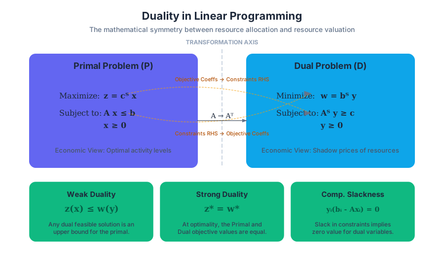
Applied Optimization: The Diet Problem
Key concepts: Cost Minimization · Nutritional Constraints · Standard Form Conversion · Real-world Modeling
A classic application of linear programming to minimize costs while meeting nutritional requirements.
Applied Optimization: The Diet Problem
The Diet Problem is a foundational archetype in the field of Linear Programming (LP) and operations research. Originally formulated in the 1930s and famously analyzed by Nobel laureate George Stigler in 1945, the problem seeks to identify the most cost-effective combination of foods that satisfies a specific set of nutritional requirements. While it may appear trivial in a modern context of abundance, the Diet Problem represents the birth of systematic resource allocation and remains the template for industrial blending, logistics, and supply chain optimization.
1. The Mathematical Foundation
At its core, the Diet Problem is a constrained optimization problem. We aim to minimize a linear cost function subject to a system of linear inequalities representing nutritional floors (and sometimes ceilings).
1.1 Formal Definition
Let $n$ be the number of available food items and $m$ be the number of essential nutrients.
- Let $x_j$ be the quantity of food $j$ to be consumed (the decision variables).
- Let $c_j$ be the cost per unit of food $j$.
- Let $a_{ij}$ be the amount of nutrient $i$ contained in one unit of food $j$.
- Let $b_i$ be the minimum daily requirement of nutrient $i$.
The objective is to:
Minimize $Z = \sum_{j=1}^{n} c_j x_j$
Subject to: $\sum_{j=1}^{n} a_{ij} x_j \ge b_i$ for all $i = 1, \dots, m$ $x_j \ge 0$ for all $j = 1, \dots, n$
1.2 Why It Matters
Beyond human nutrition, this model is used in:
- Animal Feed Formulation: Creating "Least Cost Rations" for livestock.
- Chemical Blending: Mixing raw ores or chemicals to meet a specific grade at minimum cost.
- Portfolio Optimization: Selecting assets to meet a target return while minimizing risk or cost.
- Energy Grids: Balancing power sources to meet demand at the lowest price point.
2. Standard vs. Canonical Form Conversion
In computational optimization, solvers often require problems to be in a specific format. Most textbook algorithms (like the Simplex method) assume a Standard Form or Canonical Form. Understanding the distinction is critical for debugging solver errors.
| Feature | Standard Form | Canonical Form |
|---|---|---|
| Objective | Usually Maximization | Can be Min or Max |
| Constraints | All equalities ($=$) | All inequalities ($\le$ or $\ge$) |
| Variables | All non-negative ($x_i \ge 0$) | All non-negative ($x_i \ge 0$) |
| Right-Hand Side | Non-negative ($b_i \ge 0$) | No restriction |
2.1 Transformation Mechanics
To convert a Diet Problem (typically a minimization with $\ge$ constraints) into Standard Form for a Simplex solver, we apply three primary transformations:
- Minimization to Maximization: Multiply the objective function by $-1$. $\min Z \iff \max -Z$.
- Inequality to Equality: Introduce Surplus Variables ($s_i$) and Artificial Variables ($a_i$).
- For a $\ge$ constraint: $a_{i1}x_1 + \dots \ge b_i$ becomes $a_{i1}x_1 + \dots - s_i + a_i = b_i$.
- Handling Unrestricted Variables: If a variable $x$ can be negative, replace it with $x = x^+ - x^-$, where $x^+, x^- \ge 0$.
3. Implementation: Solving with PuLP
For modern applications, we use high-level modeling libraries. Below is a Python implementation using the PuLP library, which abstracts the underlying Simplex or Interior Point solvers.
import pulp

def solve_diet_problem(food_data, nutrient_requirements):
    """
    Solves the Diet Problem using the PuLP library.
    food_data: Dict of food names to their cost and nutrient profile.
    nutrient_requirements: Dict of nutrient names to their minimum levels.
    """
    # 1. Initialize the Problem
    prob = pulp.LpProblem("The_Diet_Problem", pulp.LpMinimize)

    # 2. Define Decision Variables (x_j >= 0)
    food_items = list(food_data.keys())
    food_vars = pulp.LpVariable.dicts("Food", food_items, lowBound=0, cat='Continuous')

    # 3. Define Objective Function: Minimize Total Cost
    prob += pulp.lpSum([food_data[f]['cost'] * food_vars[f] for f in food_items]), "Total_Cost"

    # 4. Define Constraints: Meet Nutritional Minimums
    nutrients = list(nutrient_requirements.keys())
    for n in nutrients:
        prob += (
            pulp.lpSum([food_data[f][n] * food_vars[f] for f in food_items]) >=
            nutrient_requirements[n],
            f"Requirement_{n}"
        )

    # 5. Solve
    status = prob.solve(pulp.PULP_CBC_CMD(msg=0))

    # 6. Extract Results
    if pulp.LpStatus[status] == 'Optimal':
        result = {v.name: v.varValue for v in prob.variables() if v.varValue > 0}
        return result, pulp.value(prob.objective)
    else:
        return None, None

# Example Usage
foods = {
    "Spinach": {"cost": 0.12, "calories": 23, "protein": 2.9},
    "Steak": {"cost": 2.50, "calories": 250, "protein": 26.0},
    "Beans": {"cost": 0.50, "calories": 130, "protein": 8.0}
}
reqs = {"calories": 2000, "protein": 50}

plan, cost = solve_diet_problem(foods, reqs)
print(f"Optimal Plan: {plan}, Total Cost: ${cost:.2f}")
4. Algorithmic Deep-Dive: The Two-Phase Simplex
Because the Diet Problem involves $\ge$ constraints, a basic Simplex method cannot start at the origin ($0,0$) because the origin violates the "minimum requirements" constraints. We must use the Two-Phase Simplex Method.
Phase I: Finding a Feasible Basis
We introduce Artificial Variables ($a_i$) to create an initial identity matrix in the tableau. We then minimize the sum of these artificial variables.
- If the minimum sum is $0$, we have found a feasible starting point for the original problem.
- If the minimum sum is $> 0$, the problem is infeasible (no combination of foods satisfies the requirements).
Phase II: Optimizing the Objective
Once a feasible corner point is found, we drop the artificial variables and proceed with the standard Simplex algorithm to find the cost-minimizing vertex.
\begin{array}{l}
\text{Initial Tableau Construction (Phase I):} \\
\begin{bmatrix}
A & -I_{surplus} & I_{artificial} & | & b \\
0 & 0 & 1 \dots 1 & | & W
\end{bmatrix} \\
\text{Where } W \text{ is the sum of artificial variables to be minimized.}
\end{array}
5. Real-World Modeling Challenges
While the mathematical model is elegant, applying it to real-world human diets reveals several "Gotchas" that senior engineers must account for.
5.1 The "Spinach Trap" (Palatability)
A raw LP model might suggest eating 40 pounds of spinach and nothing else because it is the cheapest way to get Vitamin A and Fiber. To solve this, we add Upper Bound Constraints: $x_{spinach} \le 2.0$ (limit consumption to 2 units per day).
5.2 Integer Constraints
You cannot buy $0.342$ of an egg in a grocery store. This transforms the problem into a Mixed-Integer Linear Program (MILP), which is significantly harder to solve (NP-hard) than a standard LP.
5.3 Data Retrieval
In production environments, nutritional data is rarely hardcoded. It is pulled from relational databases.
-- Fetching nutritional data for the optimization engine
SELECT
    f.food_name,
    f.unit_cost,
    n.calories_per_unit,
    n.protein_per_unit,
    n.fat_per_unit
FROM inventory AS f
JOIN nutrition_profiles AS n ON f.food_id = n.food_id
WHERE f.in_stock = 1 AND f.unit_cost IS NOT NULL;
6. Worked Example: The "Mini-Diet"
Let's solve a manual iteration for a simplified case.
Data:
| Food | Cost ($) | Energy (kcal) | Protein (g) |
|---|---|---|---|
| Oatmeal | 0.30 | 150 | 5 |
| Milk | 0.40 | 100 | 8 |
| Target | Min Cost | $\ge$ 300 kcal | $\ge$ 20 g |
Step 1: Formulate Minimize $Z = 0.3x_1 + 0.4x_2$ Subject to:
- $150x_1 + 100x_2 \ge 300$ (Energy)
- $5x_1 + 8x_2 \ge 20$ (Protein)
- $x_1, x_2 \ge 0$
Step 2: Identify Vertices The feasible region is bounded by the intersection of these lines.
- Intersection of (1) and (2):
- $150x_1 + 100x_2 = 300 \implies 3x_1 + 2x_2 = 6$
- $5x_1 + 8x_2 = 20$
- Solving the system: $x_1 \approx 0.57, x_2 \approx 2.14$. Cost: $0.3(0.57) + 0.4(2.14) = \text{\textdollar}1.027$
- Intercepts:
- $x_1$ intercept (where $x_2=0$): $\max(300/150, 20/5) = 4$. Cost: $0.3(4) = \text{\textdollar}1.20$
- $x_2$ intercept (where $x_1=0$): $\max(300/100, 20/8) = 3$. Cost: $0.4(3) = \text{\textdollar}1.20$
Conclusion: The optimal solution is to mix approximately 0.57 units of Oatmeal and 2.14 units of Milk.
7. Common Pitfalls and Error Classification
Based on standard mastery rubrics, errors in the Diet Problem usually fall into three categories:
| Error Type | Description | Example |
|---|---|---|
| Modeling Error | Incorrectly translating units or directions. | Setting a protein constraint as $\le$ instead of $\ge$. |
| Transformation Error | Failing to correctly convert to Standard Form. | Forgetting to subtract the surplus variable in a $\ge$ constraint. |
| Infeasibility Blindness | Failing to recognize when constraints are contradictory. | Requiring 3000 calories but setting a "Max Weight" constraint that allows only 1lb of celery. |
7.1 Debugging Infeasibility
If your solver returns "Infeasible," use the following checklist:
- Check Units: Are you comparing milligrams of Sodium to grams of Protein?
- Relax Constraints: Temporarily remove constraints one by one to find the "bottleneck" nutrient.
- Variable Bounds: Ensure $x_j \ge 0$ is explicitly stated; otherwise, the solver might "eat" negative food to generate nutrients.
8. Extensions: Duality and Shadow Prices
One of the most powerful aspects of the Diet Problem is its Dual.
- Primal: Find the cheapest food mix.
- Dual: Find the "value" (shadow price) of each nutrient.
The Shadow Price of a nutrient tells you how much the total cost would change if the requirement for that nutrient increased by one unit. If the shadow price of Vitamin C is high, it suggests that Vitamin C is the primary driver of your diet's cost. This is invaluable for industrial procurement—it tells the buyer exactly which nutrient-rich ingredients are worth a premium.
# Example: Running a sensitivity analysis via a CLI wrapper
$ diet-solver --input data.json --analyze-shadow-prices

Nutrient       | Shadow Price | Sensitivity Range
-------------------------------------------------
Protein        | 0.05         | [45g, 62g]
Calories       | 0.0002       | [1800, 2500]
Vitamin A      | 1.20         | [0, 5000IU]

# Insight: Vitamin A is the "bottleneck". Reducing its requirement
# by 1 unit saves $1.20.
Summary of Mastery
To achieve Mastery+ in Applied Optimization:
- Formulate the problem with clear decision variables and units.
- Convert the model between Standard, Canonical, and Slack forms without sign errors.
- Implement the solution using professional-grade libraries (PuLP, SciPy, or Gurobi).
- Interpret the results, including shadow prices and feasibility ranges, to provide actionable business or biological insights.
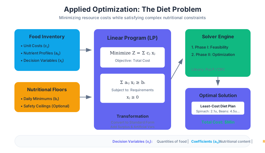
Assessment and Mastery-Based Learning
Key concepts: Mastery Rubric · Self-Reflection · Error Classification · Conceptual Understanding
Guidelines on how student performance is evaluated through rubrics and self-reflection.
Assessment and Mastery-Based Learning
Mastery-based learning (MBL) represents a paradigm shift from traditional normative grading to a competency-centric model. In the context of mathematical optimization and linear programming (LP), this approach acknowledges that "getting the right answer" is often secondary to the robustness of the underlying logic and the precision of the execution. In professional optimization environments, a single sign error in a constraint matrix can lead to an infeasible solution or, worse, a feasible but incorrect "optimal" result that costs millions in misallocated resources.
The mastery framework employed here focuses on four pillars: the Mastery Rubric, Self-Reflection, Error Classification, and Conceptual Understanding. By decoupling the learning process from the pressure of accumulating points, students are encouraged to treat errors not as failures, but as diagnostic data points for iterative improvement.
The Mastery Rubric: Defining Competence
The core of the assessment system is a non-linear 5-point scale. Unlike traditional grading where a 3/5 might represent a 60% (D-grade), in a mastery system, each level represents a qualitative state of understanding. This scale prioritizes the structural integrity of the mathematical argument over the final numerical output.
The 5-Point Mastery Scale
| Level | Designation | Description | Technical Criteria |
|---|---|---|---|
| 5 | Mastery+ | Exceptional execution | Flawless logic, optimal notation, and clear communication. The solution is "production-ready." |
| 4 | Mastery | Core competency achieved | The student demonstrates a full grasp of the concept. Minor "clerical" errors (e.g., $2+3=6$) may exist, but the strategy is sound. |
| 3 | Journeyman | Functional but fragile | The student understands the algorithm but makes significant execution errors or lacks clarity in the formal proof/derivation. |
| 2 | Apprentice | Partial understanding | The student identifies the correct method (e.g., Gauss-Jordan) but fails to apply it correctly or misses critical constraints. |
| 0-1 | No Evidence | Conceptual gap | The student either did not attempt the problem or used a fundamentally incorrect approach (e.g., treating a non-linear problem as linear). |
The Mastery Principle: A student who correctly sets up a complex Linear Programming Problem (LPP) in standard form but makes an arithmetic error in the final pivot is often closer to "Mastery" than a student who guesses the correct answer without providing a logical derivation.
Error Classification: The Taxonomy of Mistakes
To achieve mastery, one must move beyond the binary of "right vs. wrong" and into the realm of error diagnostics. In this course, errors are categorized into three distinct buckets. This classification allows students to identify whether their struggle is with the math (arithmetic), the logic (strategy), or the language (communication).
1. Strategic (Conceptual) Errors
These are the most critical. A strategic error occurs when the student misunderstands the underlying theorem or algorithm.
- Example: Failing to convert a "greater than or equal to" constraint by multiplying by $-1$ when moving to standard form.
- Impact: High. These errors invalidate the entire solution path.
2. Computational (Arithmetic) Errors
These are "low-level" errors. They occur when the student knows exactly what to do but fails in the execution of basic operations.
- Example: Adding $R_1 + R_2$ in a Gauss-Jordan elimination and getting the wrong sum in one column.
- Impact: Moderate. While the result is wrong, the student’s "Strategic Mastery" remains intact.
3. Communication (Clarity) Errors
Optimization is a collaborative field. If a model cannot be read or verified by another engineer, it is useless.
- Example: Using variables like $x, y, z$ without defining what they represent in the physical world (e.g., "let $x$ be the number of units produced").
- Impact: Variable. Crucial for professional practice and "Mastery+" designation.
Implementation: Gauss-Jordan and LPP Conversion
Mastery is best demonstrated through the foundational tools of Linear Programming: Gauss-Jordan Elimination and LPP Normalization. Before one can use the Simplex Method, one must master the transformation of systems of equations.
Standard vs. Canonical Form
In the study of Linear Programming Problems (LPPs), we distinguish between different "shapes" a problem can take. Mastery requires the ability to fluidly convert between these forms.
| Feature | Standard Form | Canonical Form |
|---|---|---|
| Objective | Maximize $Z = \mathbf{c}^T\mathbf{x}$ | Maximize $Z = \mathbf{c}^T\mathbf{x}$ |
| Constraints | All constraints are equations ($=$) | All constraints are inequalities ($\le$) |
| Variables | All variables are non-negative ($x_i \ge 0$) | All variables are non-negative ($x_i \ge 0$) |
| Right-Hand Side | $b_i$ must be non-negative | No restriction on $b_i$ sign |
The Algorithm: LPP to Standard Form
- Objective Function: If minimizing $f(x)$, convert to maximizing $-f(x)$.
- Inequalities:
- For $\sum a_{ij}x_j \le b_i$, add a slack variable $s_i$.
- For $\sum a_{ij}x_j \ge b_i$, subtract a surplus variable $e_i$.
- Unrestricted Variables: If $x_k$ is unrestricted in sign, replace it with $x_k' - x_k''$, where $x_k', x_k'' \ge 0$.
- Negative RHS: If $b_i < 0$, multiply the entire constraint by $-1$ (and flip the inequality sign before adding slack/surplus).
Code Implementation: The Computational Layer
To understand the difference between Strategic and Computational mastery, consider the implementation of a row reduction step. A student with strategic mastery knows that we must eliminate all non-zero entries in a column except for the pivot. A student with computational mastery ensures that floating-point errors do not accumulate.
Block 1: Low-Level Implementation (Python/NumPy)
This snippet demonstrates a single pivot step in the Gauss-Jordan method, the engine behind LPP solving.
import numpy as np

def pivot_element(matrix, row, col):
    """
    Performs a single pivot operation on a matrix in-place.
    Strategic Goal: Transform the column 'col' into a unit vector.
    """
    matrix = matrix.astype(float)
    pivot_val = matrix[row, col]

    if pivot_val == 0:
        raise ValueError("Cannot pivot on a zero element. Strategic Error: Invalid pivot choice.")

    # Normalize the pivot row
    matrix[row] = matrix[row] / pivot_val

    # Eliminate other entries in the column
    for r in range(len(matrix)):
        if r != row:
            factor = matrix[r, col]
            matrix[r] = matrix[r] - factor * matrix[row]

    return matrix

# Example: A 2x3 augmented matrix for a system of equations
tableau = np.array([[2, 4, 8],
                    [1, 1, 3]])

# Pivot on element (0,0)
result = pivot_element(tableau, 0, 0)
print(result)
# Output: [[1, 2, 4], [0, -1, -1]]
Block 2: Mathematical Derivation (LaTeX Pseudocode)
The transformation of a general LPP into Standard Form can be expressed as a formal mapping.
\text{Given a general LPP:} \\
\text{Optimize } Z = \sum_{j=1}^n c_j x_j \\
\text{Subject to: } \sum_{j=1}^n a_{ij} x_j \le b_i \quad (i \in I_{slack}) \\
\sum_{j=1}^n a_{ij} x_j \ge b_i \quad (i \in I_{surplus}) \\
x_j \ge 0 \quad (j \in J) \\

\text{Transformation Rule } \mathcal{T}: \\
\forall i \in I_{slack} \implies \sum a_{ij} x_j + s_i = b_i, \quad s_i \ge 0 \\
\forall i \in I_{surplus} \implies \sum a_{ij} x_j - e_i = b_i, \quad e_i \ge 0 \\
\text{If } b_i < 0 \implies \text{Multiply by } -1 \text{ before adding variables.}
Block 3: Real-World Usage (CLI/Optimization Solver)
In practice, mastery involves knowing how to interface with industry-standard solvers like GLPK (GNU Linear Programming Kit).
# Solving an LPP defined in MathProg (.mod) or MPS format
# -m: read model file
# --output: write solution to file

glpsol --math production_plan.mod --output results.txt

# Example output snippet showing the 'Mastery' of the solver:
# Status: INTEGER OPTIMAL
# Objective: z = 1450.000000 (MAXimum)
Self-Reflection: The Metacognitive Bridge
The most unique aspect of this assessment model is the Self-Reflection Worksheet. After an assignment is returned with feedback, students do not simply look at their grade. They must perform a post-mortem on their work.
The Reflection Process
- Discrepancy Analysis: Compare the submitted solution to the provided "Mastery" solution.
- Error Tagging: For every point lost, the student must tag it as Strategic, Computational, or Communication.
- Correction: Re-solve the specific sub-problem that was missed.
- Synthesis: Write a brief statement on what "Conceptual Understanding" was missing during the first attempt.
"I realized that my error in Problem 2 wasn't just a sign flip (Computational). I didn't realize that the variable $x_2$ was unrestricted, which meant my entire initial tableau was missing a column (Strategic). Next time, I will check variable bounds before setting up the matrix." — Example Student Reflection
Common Pitfalls in Mastery Learning
Even with a clear rubric, students often fall into specific traps that hinder their progress toward Mastery.
- The "Arithmetic Shield": Attributing all errors to "silly math mistakes." Often, what looks like an arithmetic error is actually a failure to organize work (Communication) or a misunderstanding of the pivot rules (Strategic).
- Notation Neglect: Using shorthand that makes sense to the student but violates formal mathematical syntax. In MBL, notation is thinking.
- Ignoring Chapter 0: Many students skip the Linear Algebra review (Gauss-Jordan, Matrix Inversion). However, LP is built entirely on these foundations. Without Chapter 0 mastery, the Simplex method becomes a "black box" rather than a logical progression.
Comparison of Error Impacts
| Error Type | Immediate Result | Long-term Consequence | Mastery Recovery Path |
|---|---|---|---|
| Computational | Wrong number | Minor frustration | Practice mental math or use verification steps |
| Strategic | Wrong logic | Fundamental misunderstanding of the domain | Re-read lecture notes; attend TA office hours |
| Communication | Unreadable work | Professional failure; inability to debug | Study formal proofs; use standard templates |
Conclusion: The Path to Professionalism
Mastery-based learning in optimization is not about perfection; it is about accountability. By forcing a distinction between different types of errors and requiring self-reflection, the system prepares students for the high-stakes environment of mathematical modeling. In the Hill Center Room 628 or via Zoom, the goal of the TA and instructor is to guide students through this iterative loop—moving from the "Apprentice" who follows recipes to the "Master" who understands the chemistry of the algorithm.
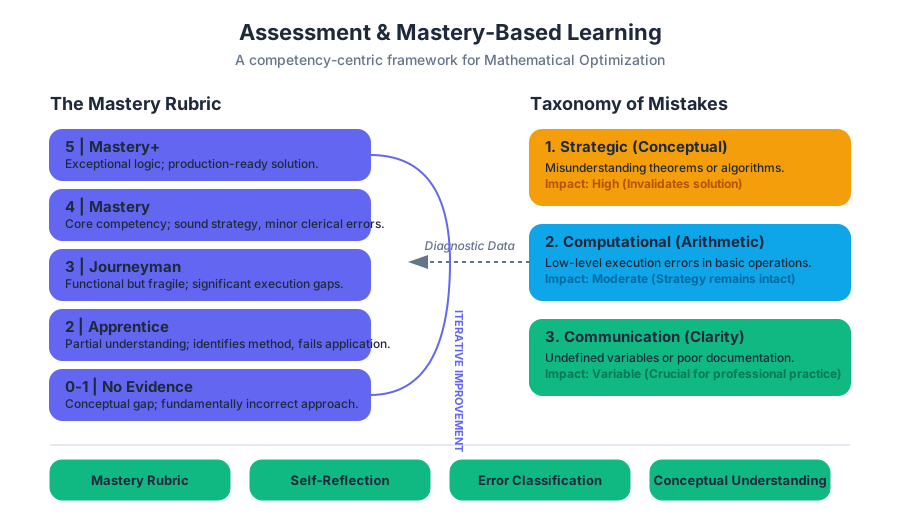
Source Materials
- Math354-Quiz1-solutions.pdf
- Math354-Quiz1.pdf
- HW1_0-5-6a.pdf
- Math354-Midterm1-solutions.pdf
- Participation4-solutions.pdf
- Math354-Participation1.pdf
- Participation1-solutions.pdf
- Math354-Participation3.pdf
- Math354-Participation6.pdf
- Math354-Participation4.pdf
- Math354-Participation5.pdf
- Math354-Participation2.pdf
Study Spring 2026 - Math 354 - Sections 02/04 with AI — Free on Lykke
Sign up for free to generate personalized flashcards, quizzes, and study guides from this course. Chat with an AI tutor that knows the material.
Get Started FreeView this course wiki on Lykke · Browse all public course wikis