Principles of Macroeconomics

Foundations of Macroeconomics and Choice

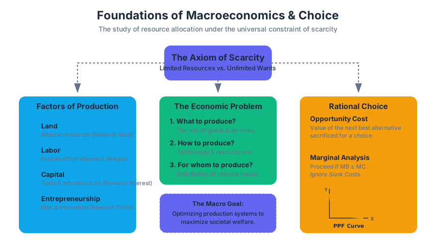
Macroeconomics is often misunderstood as the study of money, banking, and stock markets. While these are components, the core of the discipline is the study of choice under constraint. At its most fundamental level, macroeconomics seeks to understand how societies allocate limited resources to satisfy virtually unlimited human wants. This tension creates the "Economic Problem," a universal condition that necessitates trade-offs, prioritization, and the optimization of production systems.

The Axiom of Scarcity

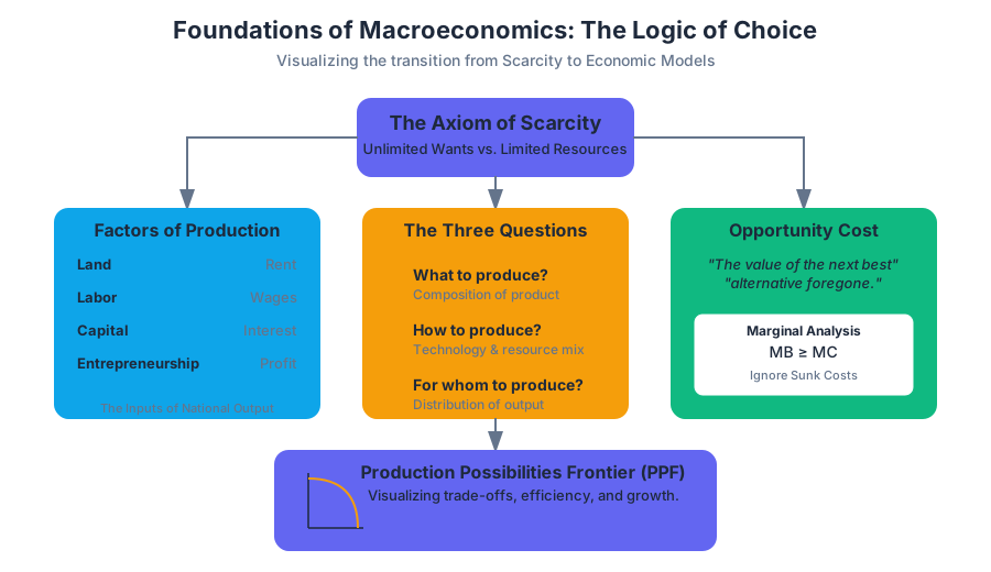
Scarcity is the foundational reality of the human condition. It is the gap between limited resources—land, labor, capital, and entrepreneurship—and the limitless desires for goods and services. Unlike a "shortage," which is a temporary market imbalance where demand exceeds supply at a specific price, scarcity is a permanent, structural fact of existence. Even the wealthiest individuals and nations face scarcity, if only in the form of time, the ultimate non-renewable resource.

The Factors of Production

To understand how scarcity manifests, we categorize the resources available to an economy into four distinct "Factors of Production."

Factor	Description	Reward/Return	Example in Macro-scale
Land	All natural resources used in production (minerals, water, arable land).	Rent	Rare earth metals for semiconductor manufacturing.
Labor	The physical and mental effort exerted by humans in production.	Wages	The aggregate workforce of a nation's tech sector.
Capital	Man-made tools, machinery, and infrastructure used to produce goods.	Interest	Automated assembly lines or fiber-optic networks.
Entrepreneurship	The human resource that organizes the other three factors and bears risk.	Profit	A startup founder developing a new carbon-capture technology.

The Mechanics of Scarcity

In a macroeconomic model, scarcity forces a society to answer three fundamental questions:

1. What to produce? (The composition of the National Product).
2. How to produce? (The choice of technology and resource mix).
3. For whom to produce? (The distribution of the resulting output).

The inability to satisfy all wants simultaneously implies that every choice to produce "Good A" is implicitly a choice not to produce "Good B." This leads us directly to the concept of the "shadow price" of all economic activity: Opportunity Cost.

Opportunity Cost: The Logic of Foregone Alternatives

Opportunity Cost is defined as the value of the next best alternative that must be sacrificed to pursue a certain action. It is not the sum of all rejected alternatives, but specifically the value of the single best alternative.

Definition: The Opportunity Cost ($OC$) of choosing alternative $A$ over $B$ is the net benefit of $B$ that is lost by not choosing it. Mathematically, if $U(x)$ is the utility or value of an option: $OC_A = U(B_{max}) - U(A)$ (where $B_{max}$ is the best alternative).

Marginal Analysis and Sunk Costs

Economists utilize Marginal Analysis to make rational decisions. This involves comparing the Marginal Benefit (MB) of an action against its Marginal Cost (MC). A rational actor continues an activity as long as $MB \geq MC$.

Crucially, this analysis ignores Sunk Costs—costs that have already been incurred and cannot be recovered. In macroeconomics, focusing on sunk costs (e.g., continuing to fund a failing infrastructure project simply because "we've already spent billions") is considered an irrational "Sunk Cost Fallacy."

# A simple Python implementation of a Resource Allocation Optimizer
# This script calculates the optimal distribution of a limited budget 
# across two competing projects based on their Marginal Benefit.

import numpy as np
from scipy.optimize import minimize

def objective_function(x):
    # We want to maximize total benefit, so we minimize the negative benefit
    # Project A benefit: sqrt(x[0]), Project B benefit: 2 * log(x[1] + 1)
    return -(np.sqrt(x[0]) + 2 * np.log(x[1] + 1))

def constraint(x):
    # Total budget constraint: x[0] + x[1] <= 100 units
    return 100 - (x[0] + x[1])

# Initial guess
x0 = [50, 50]

# Define the constraint dictionary
con = {'type': 'ineq', 'fun': constraint}

# Run the optimizer
solution = minimize(objective_function, x0, constraints=con, bounds=[(0, 100), (0, 100)])

print(f"Optimal Allocation - Project A: {solution.x[0]:.2f}, Project B: {solution.x[1]:.2f}")
print(f"Total Maximum Benefit: {-solution.fun:.2f}")

The Production Possibilities Frontier (PPF)

The Production Possibilities Frontier (PPF) is a graphical representation of the maximum possible output combinations an economy can achieve given its fixed resources and technology. It serves as a visual manifestation of scarcity, trade-offs, and efficiency.

Assumptions of the PPF Model

To isolate the mechanics of the frontier, we assume:

1. Only two goods are produced (e.g., "Capital Goods" vs. "Consumption Goods").
2. The quantity and quality of resources are fixed.
3. Technology is constant.
4. Resources are used with maximum efficiency.

The Law of Increasing Opportunity Cost

Most PPF curves are "bowed outward" (concave to the origin). This shape reflects the Law of Increasing Opportunity Cost, which states that as you produce more of one good, the opportunity cost of producing an additional unit increases. This happens because resources are not perfectly adaptable to all uses; a skilled software engineer is highly productive in "Tech Services" but may be significantly less efficient in "Agriculture."

\text{Marginal Rate of Transformation (MRT)} = \left| \frac{dY}{dX} \right|

The MRT is the slope of the PPF at any given point. It represents the rate at which one good can be "transformed" into another by reallocating resources.

Point Location	Economic Status	Meaning
On the Curve	Productive Efficiency	Resources are fully utilized; no more of one good can be produced without losing some of the other.
Inside the Curve	Inefficiency / Unemployment	Resources are idle or misallocated (e.g., high unemployment during a recession).
Outside the Curve	Unattainable (Current)	The economy lacks the resources or technology to reach this level of production.

Shifting the Frontier: Economic Growth

The PPF is not static. It can shift outward or inward based on changes in the economy’s underlying capacity.

• Outward Shift (Growth): Caused by technological advancement, discovery of new resources, or an increase in the labor force/human capital.
• Inward Shift (Contraction): Caused by natural disasters, war, or depletion of resources.

Specialization and the Gains from Trade

If scarcity limits what a single entity can produce, how do modern societies achieve such high standards of living? The answer lies in Specialization and Trade.

Absolute vs. Comparative Advantage

The distinction between these two concepts is the most critical insight in international trade theory.

1. Absolute Advantage: The ability to produce more of a good than a competitor using the same amount of resources.
2. Comparative Advantage: The ability to produce a good at a lower opportunity cost than a competitor.

The Ricardian Insight: Even if Country A has an absolute advantage in everything, it still benefits from trading with Country B, provided they have different comparative advantages. Both countries can consume at a point outside their individual PPFs by specializing in what they do relatively best and trading for the rest.

Calculating Comparative Advantage: A Numeric Example

Consider two countries, Alpha and Beta, producing Wheat and Computers with 100 units of labor.

Country	Wheat (Max Output)	Computers (Max Output)	OC of 1 Wheat	OC of 1 Computer
Alpha	100	50	0.5 Computers	2 Wheat
Beta	40	40	1 Computer	1 Wheat

In this scenario:

• Alpha has an Absolute Advantage in both Wheat and Computers.
• Alpha has a Comparative Advantage in Wheat (0.5 < 1).
• Beta has a Comparative Advantage in Computers (1 < 2).

By specializing, Alpha produces only Wheat and Beta produces only Computers. They then trade at a price (Terms of Trade) between their internal opportunity costs (e.g., 1 Wheat for 0.75 Computers).

-- Conceptual SQL query to identify trade opportunities
-- based on unit labor costs across different regions.

SELECT 
    region_name,
    product_name,
    unit_labor_cost,
    (unit_labor_cost / SUM(unit_labor_cost) OVER (PARTITION BY region_name)) AS relative_cost_index
FROM 
    regional_production_stats
WHERE 
    year = 2023
ORDER BY 
    relative_cost_index ASC;
-- Low relative_cost_index indicates a potential Comparative Advantage.

Common Pitfalls and Misconceptions

1. Confusing "Money Cost" with "Economic Cost": Students often forget that time and effort are costs. If a "free" concert requires waiting in line for 5 hours, the cost is not zero; it is the value of those 5 hours (e.g., lost wages or study time).
2. The "Fixed Pie" Fallacy: The belief that for one person/nation to gain, another must lose. Comparative advantage proves that trade is a "positive-sum game" where the total "pie" of global production increases through specialization.
3. Efficiency vs. Equity: The PPF shows Productive Efficiency (maximum output), but it does not tell us which point on the curve is "best." That is a question of Allocative Efficiency, which depends on societal preferences and values (Normative Economics).
4. Static vs. Dynamic Analysis: Assuming that a country's comparative advantage is permanent. In reality, nations can "create" comparative advantage through strategic investment in education and infrastructure (e.g., South Korea's transition from agriculture to high-tech electronics).

Synthesis: The Macroeconomic Perspective

The foundations of choice—scarcity, opportunity cost, and the PPF—provide the scaffolding for all macroeconomic theory. When we scale these individual choices up to the national level, we begin to see the mechanisms of the Circular Flow Model.

In the macro-economy:

• Households own the factors of production and sell them to firms in the Factor Market.
• Firms use these factors to produce goods and services, which they sell to households in the Product Market.
• Government intervenes to correct market failures, provide public goods, and redistribute income, effectively shifting the economy's position on or toward the PPF.

Understanding these foundations is not merely an academic exercise; it is the prerequisite for analyzing complex issues like inflation, unemployment, and global trade wars. By recognizing that every policy has an opportunity cost and every growth spurt requires an expansion of the frontier, we can move from emotive reactions to rigorous economic reasoning.

Market Mechanics and Macroeconomic Goals

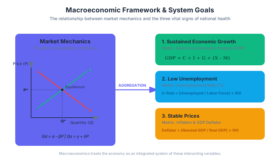
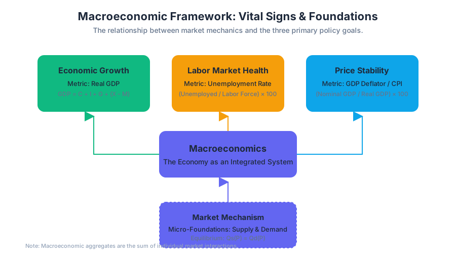
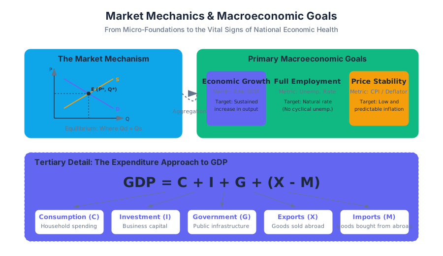
Macroeconomics is the study of the economy as an integrated system. Unlike microeconomics, which examines the decisions of individual agents, macroeconomics focuses on aggregate variables—the "vital signs" of a nation's health. To understand these signs, we must first master the underlying mechanics of market interaction and the specific metrics used to quantify progress toward three primary goals: sustained economic growth, low unemployment, and stable prices.

Supply and Demand: The Micro-Foundations of Macro

At the core of every macroeconomic aggregate lies the Market Mechanism, specifically the model of Supply and Demand. This model describes how the interaction between producers and consumers determines the Equilibrium Price ($P^$) and Equilibrium Quantity ($Q^$) of a good or service.

The Law of Demand and Supply

The Law of Demand states that, ceteris paribus (all other things being equal), as the price of a good increases, the quantity demanded decreases. Conversely, the Law of Supply posits that as the price increases, the quantity supplied increases.

Definition: Market Equilibrium A state where the quantity demanded ($Q_d$) equals the quantity supplied ($Q_s$). Mathematically, this is the intersection of the demand function $D(P)$ and the supply function $S(P)$.

Mathematical Derivation of Equilibrium

Consider a linear market model:

1. Demand Function: $Q_d = \alpha - \beta P$
2. Supply Function: $Q_s = \gamma + \delta P$

To find the equilibrium price ($P^$), we set $Q_d = Q_s$: $$\alpha - \beta P = \gamma + \delta P$$ $$\alpha - \gamma = P(\delta + \beta)$$ $$P^ = \frac{\alpha - \gamma}{\delta + \beta}$$

Once $P^$ is found, substitute it back into either equation to find $Q^$.

Worked Example: Solving a Market System

In a specialized labor market for software engineers, suppose:

• $Q_d = 500 - 5P$
• $Q_s = 100 + 3P$ (where $P$ is the hourly wage in dollars).

Setting them equal: $500 - 5P = 100 + 3P \implies 400 = 8P \implies P^* = 50$. The equilibrium quantity is $Q^* = 500 - 5(50) = 250$ engineers.

import numpy as np
from scipy.optimize import fsolve

def market_system(p, alpha, beta, gamma, delta):
    """
    Calculates the difference between supply and demand.
    At equilibrium, this function returns 0.
    """
    qd = alpha - beta * p
    qs = gamma + delta * p
    return qd - qs

# Parameters
params = {
    'alpha': 500, # Max demand at P=0
    'beta': 5,    # Demand sensitivity
    'gamma': 100, # Min supply at P=0
    'delta': 3    # Supply sensitivity
}

# Solve for P* using fsolve starting from an initial guess of 10
p_equilibrium = fsolve(market_system, x0=10, args=(params['alpha'], params['beta'], params['gamma'], params['delta']))[0]
q_equilibrium = params['alpha'] - params['beta'] * p_equilibrium

print(f"Equilibrium Price: ${p_equilibrium:.2f}")
print(f"Equilibrium Quantity: {q_equilibrium:.2f} units")

Gross Domestic Product (GDP): Measuring Economic Output

Gross Domestic Product (GDP) is the total market value of all final goods and services produced within a country's borders in a specific time period. It is the primary metric for Economic Growth.

The Expenditure Approach

The most common way to calculate GDP is the expenditure approach, which sums the spending of four sectors: $$GDP = C + I + G + (X - M)$$

Component	Symbol	Description
Consumption	$C$	Household spending on durable and non-durable goods and services.
Investment	$I$	Business spending on equipment, structures, and changes in inventories.
Government	$G$	Government spending on goods and services (excludes transfer payments).
Net Exports	$NX$	Exports ($X$) minus Imports ($M$).

Real vs. Nominal GDP

Nominal GDP measures output using current prices, while Real GDP adjusts for inflation by using constant prices from a base year. This distinction is critical: an increase in Nominal GDP could be caused by rising prices (inflation) rather than an increase in actual production.

The GDP Deflator The ratio of Nominal GDP to Real GDP, used to measure the level of prices of all new, domestically produced, final goods and services in an economy. $$GDP\ Deflator = \left( \frac{Nominal\ GDP}{Real\ GDP} \right) \times 100$$

Limitations of GDP

While a powerful metric, GDP has significant blind spots:

• Non-market transactions: Housework and volunteer work are excluded.
• The Underground Economy: Unreported income and illegal activities.
• Environmental Externalities: GDP counts the production of goods but ignores the pollution generated.
• Income Inequality: GDP per capita is an average and does not show how wealth is distributed.

Unemployment: The Human Capital Metric

The Unemployment Rate measures the health of the labor market. It represents the percentage of the labor force that is jobless, actively seeking work, and available to take a job.

Calculation and Definitions

The population is divided into three categories:

1. Employed: Currently working for pay.
2. Unemployed: Out of work but actively looking (within the last 4 weeks).
3. Out of the Labor Force: Not working and NOT looking (students, retirees, discouraged workers).

$$Unemployment\ Rate = \frac{Unemployed}{Employed + Unemployed} \times 100$$

Types of Unemployment

Economic theory distinguishes between different causes of joblessness:

Type	Cause	Economic Context
Frictional	Time spent searching for a job or transitioning between jobs.	Natural and healthy in a flexible economy.
Structural	Mismatch between worker skills and employer requirements.	Often caused by technological change or globalization.
Cyclical	Lack of aggregate demand during a recession.	The primary focus of stabilization policy.

The Natural Rate of Unemployment

The Natural Rate of Unemployment ($u^*$) is the sum of frictional and structural unemployment. When the economy is at "Full Employment," cyclical unemployment is zero, but the natural rate remains.

% Mathematical representation of the Labor Force Participation Rate (LFPR)
LFPR = \frac{Labor\ Force}{Total\ Adult\ Population} \times 100

% Okun's Law: The relationship between unemployment and GDP growth
\frac{\Delta Y}{Y} = k - c \Delta u
% Where Y is output, u is the unemployment rate, and k, c are constants.

Inflation: The Stability of Value

Inflation is a general increase in prices and a corresponding fall in the purchasing power of money. It is not an increase in the price of a single good, but a rise in the overall price level.

Measuring Inflation: The Consumer Price Index (CPI)

The CPI is calculated by tracking the price of a "basket of goods" representing the average consumer's purchases.

1. Select a Base Year: Assign it a value of 100.
2. Calculate Basket Cost: $\sum (Price_i \times Quantity_i)$ for all items in the basket.
3. Compute Index: $CPI_t = \frac{Cost\ in\ Year\ t}{Cost\ in\ Base\ Year} \times 100$.
4. Calculate Inflation Rate: $\pi = \frac{CPI_t - CPI_{t-1}}{CPI_{t-1}} \times 100$.

The Quantity Theory of Money

Economists often explain long-run inflation using the Equation of Exchange: $$M \cdot V = P \cdot Y$$ Where:

• $M$ = Money Supply
• $V$ = Velocity of Money (how fast money changes hands)
• $P$ = Price Level
• $Y$ = Real Output (Real GDP)

If $V$ and $Y$ are relatively stable, an increase in $M$ (Money Supply) leads directly to an increase in $P$ (Inflation).

Inflation Indices Comparison

Index	Scope	Primary Use
CPI	Consumer goods/services	Cost-of-living adjustments (COLAs).
PPI	Wholesale prices for producers	Early warning sign for future CPI changes.
PCE	Personal Consumption Expenditures	Preferred metric for the Federal Reserve.
Core Inflation	CPI minus Food and Energy	Measures underlying long-term trends.

-- Querying a historical economic database to find 
-- the Year-over-Year (YoY) Inflation Rate
WITH AnnualCPI AS (
    SELECT 
        reporting_year,
        AVG(index_value) as avg_cpi
    FROM economic_indicators
    WHERE indicator_name = 'CPI-U'
    GROUP BY reporting_year
)
SELECT 
    curr.reporting_year,
    curr.avg_cpi,
    prev.avg_cpi AS prev_year_cpi,
    ((curr.avg_cpi - prev.avg_cpi) / prev.avg_cpi) * 100 AS inflation_rate_yoy
FROM AnnualCPI curr
JOIN AnnualCPI prev ON curr.reporting_year = prev.reporting_year + 1
ORDER BY curr.reporting_year DESC;

Synthesis: The Phillips Curve and Policy Trade-offs

The relationship between these goals is often characterized by trade-offs. The Phillips Curve historically suggested an inverse relationship between inflation and unemployment: as unemployment falls, inflation tends to rise (due to wage pressure).

The AD-AS Model

Macroeconomists use the Aggregate Demand (AD) and Aggregate Supply (AS) model to visualize these interactions.

• AD: Total spending in the economy at different price levels.
• AS: Total production in the economy at different price levels.

A shift in AD to the right (increased spending) increases GDP and reduces unemployment but puts upward pressure on prices (inflation). Conversely, a "Supply Shock" (like an oil price spike) can shift AS to the left, causing Stagflation—a nightmare scenario of both high inflation and high unemployment.

Summary of Macroeconomic Goals

Goal	Ideal State	Metric	Primary Tool
Growth	2-3% Annual Increase	Real GDP	Investment/Innovation
Low Unemployment	4-5% (Natural Rate)	U-3 Rate	Labor Market Policy
Price Stability	2% Target Inflation	CPI / PCE	Monetary Policy

Common Pitfalls and Misconceptions

1. Confusing Stock and Flow: GDP is a flow (measured over a year), while national wealth is a stock (measured at a point in time). A country can have high GDP but be depleting its wealth (natural resources).
2. The "Lump of Labor" Fallacy: The incorrect belief that there is a fixed amount of work to be done. In reality, as the economy grows, new jobs are created, meaning technology does not inherently cause permanent unemployment.
3. Inflation vs. Relative Price Changes: If the price of iPhones goes up but the price of Androids goes down, that is a relative price change, not inflation. Inflation is a simultaneous rise in the average of all prices.
4. Real vs. Nominal Interest Rates: Borrowers and lenders must account for inflation. The Fisher Equation states: $r = i - \pi$ (Real interest rate = Nominal rate - Inflation). If you earn 5% interest but inflation is 6%, your purchasing power actually decreased by 1%.

Macroeconomic Models and Perspectives

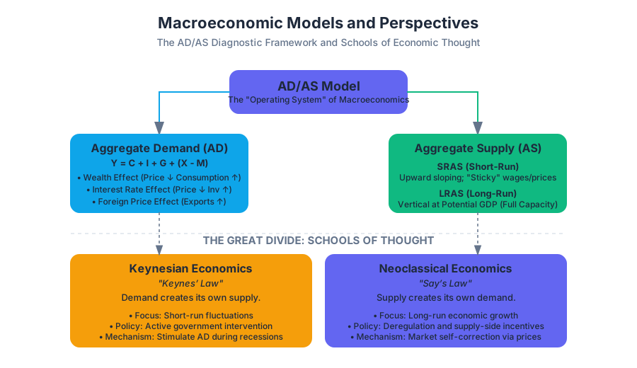
Macroeconomics is the study of the economy as a holistic, complex system. Unlike microeconomics, which focuses on individual decision-making units, macroeconomics examines the aggregate outcomes of these decisions—total output, general price levels, and systemic employment. To navigate this complexity, economists utilize the Aggregate Demand/Aggregate Supply (AD/AS) model as a primary diagnostic framework. This model serves as the "operating system" for macroeconomic analysis, providing a structured way to visualize how various shocks and policy interventions ripple through the global economy.

The field is characterized by a fundamental tension between two primary schools of thought: Keynesian Economics, which emphasizes the role of demand and the necessity of government intervention during downturns, and Neoclassical Economics, which prioritizes supply-side factors and the long-term self-correcting nature of markets. Understanding these perspectives requires a deep dive into Say’s Law, Keynes’ Law, and the mechanics of price flexibility.

The AD/AS Model: The Macroeconomic Operating System

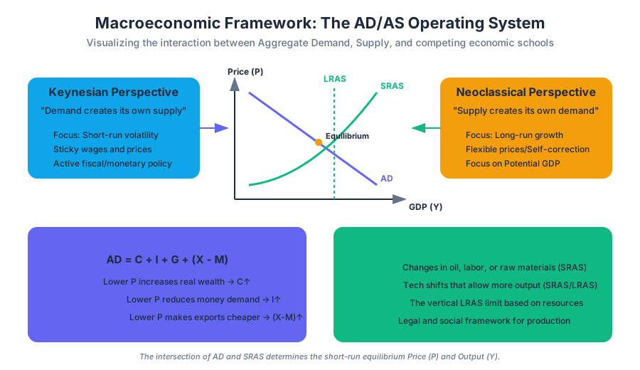
The Aggregate Demand/Aggregate Supply (AD/AS) model illustrates the relationship between the total quantity of goods and services that households, businesses, the government, and foreign buyers want to purchase (Aggregate Demand) and the total quantity that firms are willing to produce (Aggregate Supply) at a given price level.

1. Aggregate Demand (AD)

Aggregate Demand represents the total spending on domestic goods and services in an economy. It is mathematically defined by the components of Gross Domestic Product (GDP):

Definition: $AD = C + I + G + (X - M)$ Where $C$ is Consumption, $I$ is Investment, $G$ is Government Spending, $X$ is Exports, and $M$ is Imports.

The AD curve is downward-sloping due to three distinct economic phenomena:

1. The Wealth Effect: As the price level drops, the real value of money holdings increases, boosting consumer purchasing power and consumption ($C$).
2. The Interest Rate Effect: Lower price levels reduce the demand for money, leading to lower interest rates, which stimulates investment ($I$).
3. The Foreign Price Effect: If domestic prices fall while foreign prices remain constant, domestic goods become more competitive, increasing exports ($X$) and decreasing imports ($M$).

2. Aggregate Supply (AS)

Aggregate Supply refers to the total quantity of output firms are willing to produce and sell. It is divided into two distinct time horizons:

• Short-Run Aggregate Supply (SRAS): Upward-sloping because some nominal input prices (like wages) are "sticky" or slow to adjust.
• Long-Run Aggregate Supply (LRAS): A vertical line at the level of Potential GDP (also called full-employment GDP). This represents the maximum output an economy can sustain with its existing levels of labor, physical capital, technology, and institutions.

Component	Definition	Determinants of Shifts
AD	Total spending on GDP	Consumer confidence, interest rates, tax policy, government spending, exchange rates.
SRAS	Total production in the short run	Input prices (oil, labor), productivity shocks, inflation expectations, supply chain integrity.
LRAS	Potential output at full capacity	Technological innovation, growth in labor force, capital accumulation, institutional quality.

Implementation: Numerical Equilibrium Solver

In professional economic modeling, we often treat the AD/AS framework as a system of non-linear equations. The following Python implementation uses a root-finding algorithm to determine the equilibrium price level ($P$) and real output ($Y$) given specific parameters for demand and supply.

import numpy as np
from scipy.optimize import fsolve

def economy_system(vars, params):
    """
    Solves for Equilibrium Price (P) and Output (Y).
    vars: (P, Y)
    params: dictionary of exogenous variables
    """
    P, Y = vars
    
    # Aggregate Demand Equation: Y = (A - bP) / (1 - m)
    # Simplified linear form for demonstration
    ad_eq = Y - (params['autonomous_spending'] - params['price_sensitivity_ad'] * P)
    
    # Short-Run Aggregate Supply: Y = Y_pot + alpha * (P - P_expected)
    sras_eq = Y - (params['y_potential'] + params['price_sensitivity_as'] * (P - params['p_expected']))
    
    return [ad_eq, sras_eq]

# Economic Parameters
market_params = {
    'autonomous_spending': 5000,
    'price_sensitivity_ad': 15.0,
    'y_potential': 4000,
    'price_sensitivity_as': 25.0,
    'p_expected': 100
}

# Initial guess: P=100, Y=4000
initial_guess = [100, 4000]
equilibrium_p, equilibrium_y = fsolve(economy_system, initial_guess, args=(market_params,))

print(f"Equilibrium Price Level (P*): {equilibrium_p:.2f}")
print(f"Equilibrium Real GDP (Y*): {equilibrium_y:.2f}")

The Great Divide: Say’s Law vs. Keynes’ Law

The history of macroeconomic thought is largely a debate over which "law" governs the economy. This distinction dictates whether policy should focus on stimulating demand or incentivizing supply.

Say’s Law: "Supply Creates Its Own Demand"

Proposed by Jean-Baptiste Say in the early 19th century, this view suggests that the act of producing goods generates enough income (via wages and profits) to purchase those goods. In this world, sustained overproduction is impossible because prices and wages adjust instantly to clear markets.

• Focus: Long-run growth.
• Policy Implication: Minimize government interference; focus on deregulation and capital formation.

Keynes’ Law: "Demand Creates Its Own Supply"

Coined during the Great Depression by John Maynard Keynes, this law argues that firms produce only what they expect to sell. If aggregate demand is insufficient, firms will cut production and lay off workers, regardless of their capacity to supply.

• Focus: Short-run fluctuations (the business cycle).
• Policy Implication: Active fiscal and monetary policy to manage demand.

Feature	Say's Law (Neoclassical)	Keynes' Law (Keynesian)
Primary Driver	Supply / Production	Demand / Spending
Time Horizon	Long Run	Short Run
Price Behavior	Fully Flexible	Sticky / Rigid
Unemployment	Voluntary or Frictional	Involuntary (Cyclical)
Market State	Always clears	Can get stuck in "Recessionary Gap"

The Keynesian Perspective: Demand-Driven Dynamics

The Keynesian perspective is built on the observation that the economy does not always self-correct quickly. The central mechanism for this failure is Sticky Wages and Prices.

Why Prices are Sticky

1. Menu Costs: The literal and administrative costs of changing prices (printing new catalogs, updating software).
2. Coordination Failure: Even if everyone knows prices should fall, no single firm wants to be the first to cut wages or prices for fear of losing talent or revenue.
3. Efficiency Wage Theory: Employers pay more than the market-clearing wage to ensure productivity and loyalty, making them reluctant to cut pay during downturns.

The Expenditure Multiplier

Keynes introduced the concept of the Multiplier, where an initial change in spending leads to a more than proportionate change in GDP. This occurs because one person's spending becomes another's income, which is then partially spent again.

\text{Multiplier} = \frac{1}{1 - MPC(1 - t) + MPI}

• MPC: Marginal Propensity to Consume
• t: Tax rate
• MPI: Marginal Propensity to Import

Mathematical Derivation of the Multiplier Effect

% Derivation of the Equilibrium Output in a closed economy
Y = C + I + G
C = C_0 + c(Y - T)  % Consumption function with marginal propensity 'c'
Y = C_0 + c(Y - T) + I + G
Y - cY = C_0 - cT + I + G
Y(1 - c) = C_0 - cT + I + G
Y = \frac{1}{1 - c} [C_0 - cT + I + G]

% The term 1/(1-c) is the multiplier.
% If c = 0.8, the multiplier is 1/(1-0.8) = 5.

The Neoclassical Perspective: Supply-Side Fundamentals

Neoclassical economists argue that while demand-side shocks matter in the short run, the economy's long-run trajectory is determined by its productive capacity (LRAS). They emphasize the role of Rational Expectations.

1. Rational Expectations vs. Adaptive Expectations

• Adaptive Expectations: People look at past trends to predict the future. If inflation was 2% last year, they expect 2% this year.
• Rational Expectations: People use all available information, including predicted government policy, to form forecasts. If the government announces a stimulus that will cause inflation, people adjust their behavior (and prices) immediately.

2. The Self-Correcting Mechanism

In the neoclassical view, if the economy is in a recession, the surplus of labor will eventually drive down wages. Lower wages reduce production costs, shifting the SRAS curve to the right until the economy returns to Potential GDP.

3. Policy Focus: The "Natural Rate"

Neoclassical policy focuses on reducing the Natural Rate of Unemployment (frictional + structural) rather than trying to eliminate cyclical unemployment through demand management, which they believe only leads to inflation in the long run.

Synthesis: The Modern Macroeconomic Consensus

Modern macroeconomics often uses a "Keynesian in the short run, Neoclassical in the long run" approach. This synthesis acknowledges that while demand management is necessary to mitigate immediate crises, long-term prosperity depends on supply-side factors like education, infrastructure, and technology.

Comparison of Policy Tools

Tool	Keynesian Application	Neoclassical Application
Fiscal Policy	Deficit spending to boost AD during recessions.	Tax cuts to incentivize investment and work.
Monetary Policy	Lowering interest rates to stimulate $I$ and $C$.	Maintaining low, predictable inflation to reduce uncertainty.
Labor Market	Minimum wage and unions to protect worker income.	Flexible wages and labor mobility to ensure market clearing.

Real-World Application: Analyzing Economic Data

To apply these models, economists fetch real-time data from sources like the Federal Reserve Economic Data (FRED). Below is a conceptual example of how an analyst might use a CLI tool or script to pull GDP and Price Level data to determine where an economy sits relative to its LRAS.

# Example: Fetching Real GDP and GDP Deflator via a hypothetical API CLI
# This represents the data gathering phase for AD/AS analysis

# 1. Get Real GDP (Output Y)
curl -X GET "https://api.stlouisfed.org/fred/series/observations?series_id=GDPC1&api_key=your_key" \
     -H "Accept: application/json" > real_gdp.json

# 2. Get GDP Deflator (Price Level P)
curl -X GET "https://api.stlouisfed.org/fred/series/observations?series_id=GDPDEF&api_key=your_key" \
     -H "Accept: application/json" > price_level.json

# 3. Analyze the output: If Real GDP < Potential GDP (GDPC1 < GDPPOT), 
# the economy is in a recessionary gap.

Common Pitfalls and Misconceptions

• Confusing Micro-Supply with Macro-Supply: In microeconomics, a supply curve slopes up because of substitution (producing more of X instead of Y). In macroeconomics, the SRAS slopes up because of economy-wide nominal rigidities (wages/prices).
• The "Lump of Labor" Fallacy: The mistaken belief that there is a fixed amount of work to be done. Neoclassical theory refutes this, showing that supply creates its own demand through the circular flow of income.
• Ignoring the Time Lag: Keynesian policy often suffers from "recognition lags" (realizing there is a problem) and "implementation lags" (passing legislation), which can lead to stimulus hitting the economy only after it has already begun to recover.

Monetary and Fiscal Policy

Overview

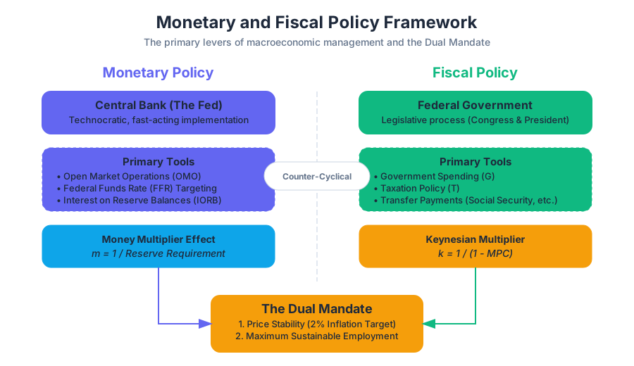
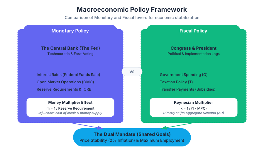
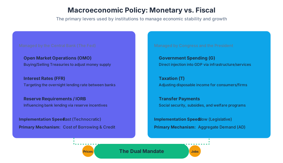
In the theater of macroeconomics, two primary levers control the speed and direction of the national economy: Monetary Policy and Fiscal Policy. While they share the ultimate goal of maintaining price stability and full employment—often referred to as the "Dual Mandate" in the United States—they operate through fundamentally different mechanisms, timelines, and institutions.

Monetary policy is the domain of the central bank (the Federal Reserve), focusing on the management of the money supply and interest rates. Fiscal policy is the domain of the federal government (Congress and the President), focusing on government spending and taxation. Together, these tools form the basis of counter-cyclical management, attempting to smooth out the "boom and bust" cycles of the market.

Monetary Policy: The Central Bank’s Toolkit

Monetary Policy refers to the actions taken by a central bank to influence the availability and cost of money and credit. In the United States, the Federal Reserve (the "Fed") uses these tools to steer the economy toward its goals of maximum employment and stable prices (typically targeted at 2% inflation).

The Mechanics of the Federal Reserve

The Fed does not directly set the interest rate you pay on a car loan. Instead, it targets the Federal Funds Rate (FFR)—the interest rate at which commercial banks lend their excess reserves to each other overnight. By moving this "anchor" rate, the Fed creates a ripple effect throughout the entire yield curve.

The Money Multiplier Effect: The process by which the banking system creates money. When a bank receives a deposit, it keeps a fraction (the Reserve Requirement) and lends out the rest. The formula for the maximum money multiplier ($m$) is: $$m = \frac{1}{RR}$$ where $RR$ is the reserve requirement ratio.

Tools of Monetary Policy

Historically, the Fed utilized three primary tools, though modern "Ample Reserves" frameworks have shifted the emphasis toward interest on reserve balances.

Tool	Action	Impact on Money Supply	Impact on Interest Rates
Open Market Operations (OMO)	Buying/Selling Treasury bonds	Buying increases supply	Decreases rates
Discount Rate	Interest rate charged to banks by the Fed	Lowering increases borrowing	Decreases market rates
Reserve Requirements	% of deposits banks must hold	Lowering increases lending	Decreases rates
Interest on Reserve Balances (IORB)	Paying banks to keep money at the Fed	Increasing decreases lending	Increases market rates

Implementation: The Taylor Rule

Central bankers often use a heuristic known as the Taylor Rule to determine the optimal Federal Funds Rate based on current inflation and the "output gap" (the difference between actual GDP and potential GDP).

# A Python implementation of the Taylor Rule for Interest Rate Targeting
def calculate_taylor_rule(neutral_rate, current_inflation, target_inflation, 
                         gdp_gap, weight_inflation=0.5, weight_gdp=0.5):
    """
    Calculates the suggested Federal Funds Rate.
    
    Parameters:
    neutral_rate (float): The real equilibrium fed funds rate (r*)
    current_inflation (float): Current CPI or PCE inflation rate
    target_inflation (float): The central bank's inflation target (usually 2.0)
    gdp_gap (float): (Actual GDP - Potential GDP) / Potential GDP * 100
    """
    
    # The standard Taylor Rule formula:
    # r = pi + 0.5(pi - pi*) + 0.5(y_gap) + r*
    
    inflation_gap = current_inflation - target_inflation
    
    suggested_rate = (current_inflation + 
                      weight_inflation * inflation_gap + 
                      weight_gdp * gdp_gap + 
                      neutral_rate)
    
    return round(suggested_rate, 2)

# Example: High inflation (5%) and a positive GDP gap (2%)
# Neutral rate assumed at 2%
policy_rate = calculate_taylor_rule(2.0, 5.0, 2.0, 2.0)
print(f"Suggested Federal Funds Rate: {policy_rate}%") 
# Output: 8.5% (Highly contractionary)

Fiscal Policy: Spending and Taxation

Fiscal Policy is the use of government spending ($G$) and tax policy ($T$) to influence aggregate demand ($AD$). Unlike monetary policy, which is technocratic and fast-acting, fiscal policy is inherently political and subject to significant "implementation lags" due to the legislative process.

The Keynesian Multiplier

The core justification for fiscal intervention is the Spending Multiplier. The idea is that an initial dollar of government spending becomes income for a citizen, who then spends a portion of it, creating further income for others.

The strength of this effect depends on the Marginal Propensity to Consume (MPC)—the fraction of an additional dollar of income that a household spends rather than saves.

\text{Spending Multiplier} = \frac{1}{1 - MPC}
\text{Tax Multiplier} = \frac{-MPC}{1 - MPC}

Note: The tax multiplier is always smaller than the spending multiplier because part of a tax cut is saved by households immediately, whereas government spending enters the GDP stream directly.

Expansionary vs. Contractionary Fiscal Policy

Policy Type	Goal	Tools	Effect on Budget
Expansionary	Fight Recession / Reduce Unemployment	$\uparrow G$ or $\downarrow T$	Increases Deficit
Contractionary	Reduce Inflation	$\downarrow G$ or $\uparrow T$	Increases Surplus / Reduces Deficit

Worked Example: Closing a Recessionary Gap

Suppose an economy has a GDP gap of $400 billion. The government wants to close this gap using fiscal policy, and the $MPC$ is estimated at 0.8.

1. Calculate the Multiplier: $1 / (1 - 0.8) = 5$.
2. Calculate Required Spending: $\Delta G = \text{Gap} / \text{Multiplier} = 400 / 5 = 80$.
3. Result: An injection of $80 billion in new spending will (theoretically) increase total GDP by $400 billion.

Budget Deficits and National Debt

When a government's spending ($G$) exceeds its tax revenue ($T$) in a single year, it runs a Budget Deficit. To finance this, the Treasury issues debt (Bonds, Notes, and Bills). The National Debt is the accumulation of all past deficits and surpluses.

The Crowding Out Effect

A primary criticism of large fiscal deficits is Crowding Out. When the government borrows heavily, it increases the demand for loanable funds, which can drive up interest rates. Higher interest rates make it more expensive for private firms to borrow for investment ($I$).

Crowding Out Theorem: $G \uparrow \rightarrow \text{Demand for Funds} \uparrow \rightarrow r \uparrow \rightarrow I \downarrow$ In this scenario, government spending does not add to total demand; it simply replaces private investment.

Tracking Fiscal Health

To manage these variables, economists track the Debt-to-GDP Ratio. A country with a high debt might still be "healthy" if its GDP is growing faster than its debt servicing costs.

-- A conceptual SQL schema for a National Treasury's Ledger
CREATE TABLE FiscalYear (
    year_id INT PRIMARY KEY,
    total_revenue_usd DECIMAL(18, 2), -- Tax receipts
    total_outlay_usd DECIMAL(18, 2),  -- Government spending
    gdp_nominal_usd DECIMAL(18, 2)
);

-- Calculate the annual deficit and debt-to-gdp ratio
SELECT 
    year_id,
    (total_outlay_usd - total_revenue_usd) AS annual_deficit,
    ((total_outlay_usd - total_revenue_usd) / gdp_nominal_usd) * 100 AS deficit_gdp_pct,
    -- Analytical window function to show cumulative debt
    SUM(total_outlay_usd - total_revenue_usd) OVER (ORDER BY year_id) AS national_debt
FROM FiscalYear;

Policy Coordination and Constraints

While we discuss these policies separately, they interact constantly. This interaction can be complementary or conflicting.

The Phillips Curve and Trade-offs

The Phillips Curve suggests an inverse relationship between unemployment and inflation.

• Expansionary Policy: Lowers unemployment but risks higher inflation.
• Contractionary Policy: Lowers inflation but risks higher unemployment.

Lags in Policy

Policy does not work instantaneously. Economists identify three types of lags:

1. Recognition Lag: The time it takes to realize a recession or inflation is happening (data is often backward-looking).
2. Legislative (Implementation) Lag: The time it takes for Congress to pass a bill or the Fed to meet.
3. Impact Lag: The time it takes for the money to actually circulate through the economy (often 6–18 months).

Comparison: Monetary vs. Fiscal Policy

Feature	Monetary Policy	Fiscal Policy
Decision Maker	Central Bank (The Fed)	Government (Congress/President)
Primary Tool	Interest Rates / Money Supply	Taxes / Spending
Political Influence	Low (Independent)	High (Voter-driven)
Speed of Action	Fast (Immediate implementation)	Slow (Legislative hurdles)
Main Constraint	Liquidity Trap / Zero Lower Bound	Political Gridlock / Debt Sustainability

Common Pitfalls and Misconceptions

1. The "Household" Fallacy

A common mistake is comparing a national budget to a household budget. While a household must eventually pay off its debt, a government can "roll over" debt indefinitely as long as the economy grows and it maintains the power to tax. The constraint is not "running out of money," but rather the inflationary pressure caused by over-stimulating the economy.

2. The Liquidity Trap

In a deep recession, interest rates may hit the Zero Lower Bound (ZLB). At this point, traditional monetary policy becomes ineffective because rates cannot go lower. This is when "Unconventional Monetary Policy," such as Quantitative Easing (QE)—where the Fed buys long-term assets to lower long-term rates—is employed.

3. Automatic Stabilizers

Not all fiscal policy is "discretionary." Automatic Stabilizers are programs that automatically stimulate the economy without new legislation. For example, in a recession, more people qualify for unemployment insurance (increasing $G$) and people earn less income, so they pay less in taxes (decreasing $T$). This provides an immediate, non-political cushion.

Practical Implementation: Executing a Policy Shift

In the real world, a policy shift involves a complex series of market operations. If the Fed decides to raise rates, it doesn't just change a number on a website; it conducts transactions.

# Conceptual CLI for a Central Bank Operations Desk
# Step 1: Check current reserve levels
$ fed-cli get-reserves --market=overnight

# Step 2: Conduct Open Market Sale to drain liquidity (raise rates)
$ fed-cli sell-treasuries --amount=50B --target-rate=5.25

# Step 3: Monitor the Effective Federal Funds Rate (EFFR)
$ watch fed-cli get-effr

Globalization and the Future of Economic Education

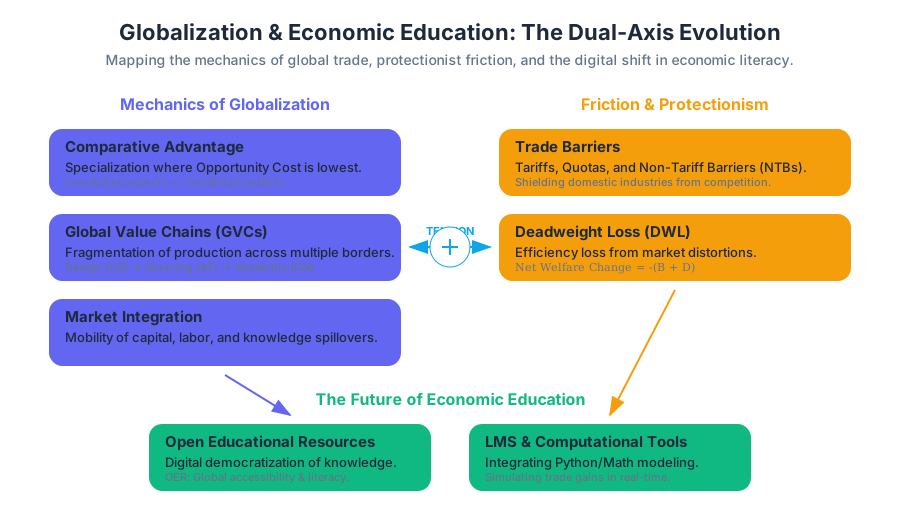
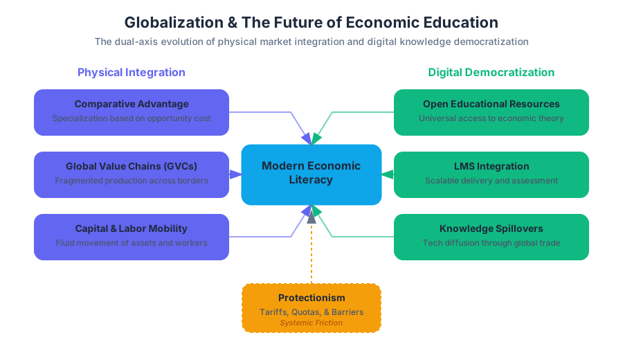
The modern economic landscape is defined by a dual-axis evolution: the physical integration of global markets and the digital democratization of economic knowledge. As national borders become increasingly porous to capital, labor, and goods, the methods by which we teach and understand these phenomena must similarly evolve. This article explores the mechanics of Globalization and Protectionism, and the technological shift toward Open Educational Resources (OER) and LMS Integration that ensures economic literacy keeps pace with global complexity.

The Mechanics of Globalization and International Trade

Globalization refers to the multidimensional process of increasing economic, social, and technological interdependence between nations. In a strictly economic sense, it is characterized by the expansion of international trade, the mobility of capital, and the integration of labor markets.

Comparative Advantage and Trade Theory

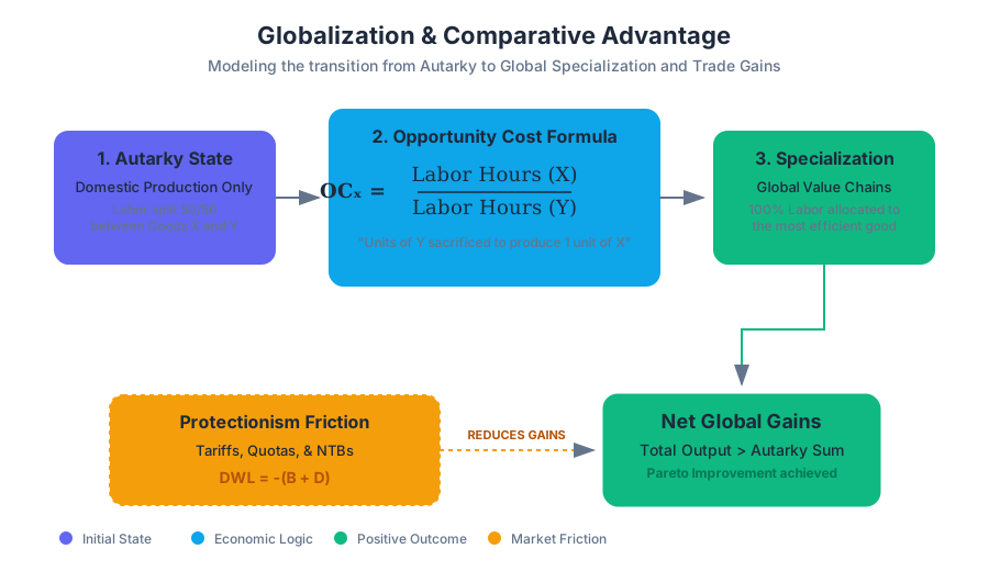
At the heart of globalization lies the principle of Comparative Advantage. Unlike absolute advantage (where one country is simply better at producing everything), comparative advantage posits that trade is mutually beneficial if countries specialize in goods where their opportunity cost is lowest.

The Law of Comparative Advantage: A nation should specialize in the production and export of goods that it can produce at a lower relative opportunity cost than its trading partners, even if it lacks an absolute advantage in those goods.

Mathematically, if Country $A$ and Country $B$ produce goods $X$ and $Y$, Country $A$ has a comparative advantage in $X$ if: $$\frac{Cost_A(X)}{Cost_A(Y)} < \frac{Cost_B(X)}{Cost_B(Y)}$$

Global Value Chains (GVCs)

Modern globalization has moved beyond the simple exchange of finished goods to the fragmentation of production across borders. A single smartphone may be designed in the US, sourced with minerals from Africa, manufactured with components from Taiwan and Germany, and assembled in China.

Concept	Description	Impact on Education
Trade Liberalization	The removal or reduction of restrictions on the free exchange of goods between nations.	Requires students to understand multilateral agreements (WTO, USMCA).
Capital Mobility	The ease with which assets can be moved across borders.	Shifts focus toward international finance and exchange rate volatility.
Labor Arbitrage	Seeking lower labor costs in foreign markets.	Drives the study of domestic wage inequality and structural unemployment.
Knowledge Spillovers	The diffusion of technology and "know-how" through trade.	Highlights the importance of Intellectual Property (IP) in economic curricula.

Implementation: Modeling Trade Gains

To understand the impact of trade, economists use computational models to simulate the shift from Autarky (self-sufficiency) to free trade.

import numpy as np

def calculate_trade_gains(labor_hours, country_a_coeffs, country_b_coeffs):
    """
    Simulates production possibilities and gains from trade.
    coeffs = [hours_per_unit_wheat, hours_per_unit_wine]
    """
    # Production in Autarky (splitting labor 50/50)
    a_wheat_aut = (labor_hours / 2) / country_a_coeffs[0]
    a_wine_aut = (labor_hours / 2) / country_a_coeffs[1]
    
    b_wheat_aut = (labor_hours / 2) / country_b_coeffs[0]
    b_wine_aut = (labor_hours / 2) / country_b_coeffs[1]
    
    # Specialization based on Comparative Advantage
    # Country A specializes in Wheat if its opportunity cost is lower
    opp_cost_a = country_a_coeffs[0] / country_a_coeffs[1]
    opp_cost_b = country_b_coeffs[0] / country_b_coeffs[1]
    
    if opp_cost_a < opp_cost_b:
        # A specializes in Wheat, B in Wine
        a_spec = [labor_hours / country_a_coeffs[0], 0]
        b_spec = [0, labor_hours / country_b_coeffs[1]]
    else:
        # A specializes in Wine, B in Wheat
        a_spec = [0, labor_hours / country_a_coeffs[1]]
        b_spec = [labor_hours / country_b_coeffs[0], 0]
        
    total_autarky = [a_wheat_aut + b_wheat_aut, a_wine_aut + b_wine_aut]
    total_specialized = [a_spec[0] + b_spec[0], a_spec[1] + b_spec[1]]
    
    gains = np.subtract(total_specialized, total_autarky)
    
    return {
        "Autarky Total": total_autarky,
        "Specialized Total": total_specialized,
        "Net Gains": gains
    }

# Example: Country A (1h Wheat, 2h Wine) vs Country B (3h Wheat, 4h Wine)
results = calculate_trade_gains(1000, [1, 2], [3, 4])
print(f"Global Gains from Trade: {results['Net Gains']}")

Protectionism: The Friction in Global Trade

While trade offers aggregate gains, it creates winners and losers within domestic economies. Protectionism encompasses policy actions intended to shield domestic industries from foreign competition.

Tools of Protectionism

1. Tariffs: Taxes imposed on imported goods, increasing their price and making domestic alternatives more attractive.
2. Import Quotas: Physical limits on the quantity of a good that can be imported.
3. Non-Tariff Barriers (NTBs): Regulatory requirements, safety standards, or "Buy Local" laws that indirectly restrict trade.
4. Export Subsidies: Financial support from the government to domestic firms to help them compete in global markets.

The Welfare Cost of Tariffs

Protectionism creates a Deadweight Loss (DWL)—a loss of economic efficiency that occurs when the equilibrium for a good or service is not achieved.

% Mathematical representation of Welfare Loss due to Tariffs
\text{Consumer Surplus Loss} = -(A + B + C + D)
\text{Producer Surplus Gain} = +A
\text{Government Revenue Gain} = +C
\text{Net Welfare Change (DWL)} = -(B + D)

\text{Where:}
B = \text{Production Distortion (Efficiency loss from inefficient domestic production)}
D = \text{Consumption Distortion (Loss from consumers who exit the market)}

Policy Tool	Primary Beneficiary	Primary Victim	Impact on Price
Tariff	Domestic Producers / Govt	Domestic Consumers	Increases
Quota	Domestic Producers / Foreign License Holders	Domestic Consumers	Increases
Subsidy	Domestic Producers	Taxpayers	Decreases (locally)
Voluntary Export Restraint (VER)	Foreign Producers (higher margins)	Domestic Consumers	Increases

The "Infant Industry" Argument

One of the most persistent justifications for protectionism is the Infant Industry Argument. It suggests that new industries in developing nations need temporary protection to develop economies of scale and expertise before they can compete with established global giants. However, critics argue these "infants" often never "grow up," leading to long-term inefficiencies and political rent-seeking.

The Democratization of Knowledge: Open Educational Resources (OER)

As the global economy becomes more complex, the cost of accessing high-quality economic education has historically risen. Open Educational Resources (OER) represent a paradigm shift, moving from proprietary, high-cost textbooks to free, openly licensed materials.

The 5Rs of OER

For a resource to be truly "Open," it must permit the following:

• Retain: The right to make, own, and control copies of the content.
• Reuse: The right to use the content in a wide range of ways.
• Revise: The right to adapt, adjust, modify, or alter the content.
• Remix: The right to combine the original or revised content with other material.
• Redistribute: The right to share copies of the original content, your revisions, or your remixes with others.

OpenStax and the OER Ecosystem

Platforms like OpenStax (from Rice University) provide peer-reviewed, professional-grade textbooks—such as Principles of Macroeconomics 3e—at no cost. This removes the "textbook barrier," where students may opt out of a course or fail because they cannot afford the required reading.

Economic Insight: OER reduces the "Price Floor" of education to zero, effectively shifting the supply curve of educational materials to the right and increasing the quantity of human capital produced.

LMS Integration: Bridging Content and Pedagogy

The future of economic education isn't just about what is taught, but how it is delivered. LMS Integration (Learning Management System) allows OER content to be embedded directly into platforms like Canvas, Blackboard, or Moodle.

LTI (Learning Tools Interoperability)

The technical standard that makes this possible is LTI. It allows a "Tool Provider" (like OpenStax Assignable) to securely communicate with a "Tool Consumer" (the university's LMS).

Benefits of Integration

• Single Sign-On (SSO): Students access all materials without separate accounts.
• Gradebook Sync: Interactive quizzes and assessments automatically update the instructor's gradebook.
• Data Analytics: Instructors can see which sections of the "textbook" students are struggling with in real-time.

Technical Configuration: LTI 1.3 JSON Example

Integrating an OER resource requires a handshake between the LMS and the content provider. Below is a conceptual JSON configuration for an LTI 1.3 tool.

{
  "title": "OpenStax Macroeconomics 3e",
  "scopes": [
    "https://purl.imsglobal.org/spec/lti-ags/scope/lineitem",
    "https://purl.imsglobal.org/spec/lti-ags/scope/result.readonly",
    "https://purl.imsglobal.org/spec/lti-nrps/scope/contextmembership.readonly"
  ],
  "extensions": [
    {
      "platform": "canvas.instructure.com",
      "settings": {
        "placements": [
          {
            "placement": "course_navigation",
            "message_type": "LtiResourceLinkRequest",
            "target_link_uri": "https://assignable.openstax.org/launch"
          }
        ]
      }
    }
  ],
  "public_jwk_url": "https://assignable.openstax.org/api/lti/jwks",
  "oidc_initiation_url": "https://assignable.openstax.org/api/lti/authorize"
}

The Future: Data-Driven and Diverse Perspectives

The integration of OER and LMS technology allows for a more dynamic curriculum. Traditional textbooks are updated every 3–5 years; OER can be updated annually or even more frequently to reflect:

• Real-time Data: Integrating FRED (Federal Reserve Economic Data) directly into the reading.
• Diverse Perspectives: Moving beyond Western-centric models to include socio-political economic ties and the impacts of trade on the Global South.
• Interactive Simulations: Using tools like the one below to visualize market shifts.

Common Pitfalls in Global Economic Education

• The Zero-Sum Fallacy: The mistaken belief that if one country gains from trade, another must lose. (Comparative advantage proves otherwise).
• Ignoring Distributional Effects: Teaching that "trade is good" without acknowledging that specific sectors (e.g., manufacturing in high-wage countries) may suffer.
• OER Quality Concerns: The misconception that "free" means "low quality." Modern OER undergoes the same rigorous peer-review process as traditional publishing.

Feature	Traditional Textbook	Open Educational Resources (OER)
Cost to Student	$100 - $300+	$0
Customizability	None (Static)	High (Remixable)
Accessibility	Limited by physical/digital DRM	Universal / High (WCAG Compliant)
Updates	New editions every few years	Continuous / Community-driven
LMS Integration	Often requires paid "Access Codes"	Native / Free via LTI

Conclusion: The Synthesis of Trade and Tech

Globalization has made the world's economies inseparable, while the OER movement is making economic knowledge inescapable. By integrating high-quality, open-source content directly into the digital workflows of students, we ensure that the next generation of policymakers, entrepreneurs, and citizens can navigate a world where the only constant is interconnected change. The future of economic education is not just about learning the laws of supply and demand—it is about leveraging open technology to ensure those laws are understood by everyone, everywhere.