Precalculus
Institution: MIT
42 study materials · 11 sections
The Client Challenge Precalculus course is a comprehensive curriculum designed to bridge the gap between high school algebra and college-level calculus. It covers ten core units ranging from composite functions and trigonometry to matrices and limits, providing a rigorous foundation in mathematical analysis. Students engage with diverse topics such as sinusoidal modeling, conic sections, and probability to develop the analytical skills necessary for advanced STEM fields.
Course Sections
Composite and Inverse Functions
Key concepts: Function Composition notation (g ∘ h)(x) · Invertible functions · Domain restriction · Verifying inverses by composition · Modeling with functions
This section introduces the mechanics of combining functions and finding their inverses, focusing on algebraic substitution, tabular analysis, and domain restrictions.
Composite and Inverse Functions
In the study of advanced algebra and precalculus, functions are often treated as static entities—mappings from a set $A$ to a set $B$. However, the true power of functional analysis emerges when we treat functions as dynamic components that can be linked, reversed, and transformed. Composite and inverse functions represent the "connective tissue" of mathematical modeling, allowing us to describe complex, multi-stage processes and backtrack from results to their original inputs.
Function Composition: The Pipeline of Mathematics
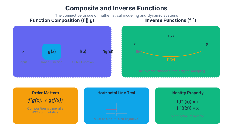
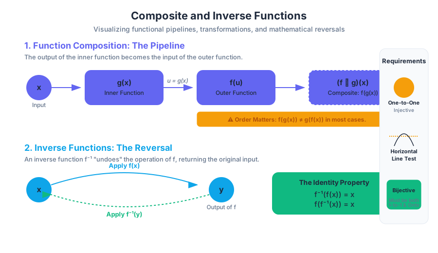
Function composition is the process of applying one function to the results of another. If we have two functions, $f$ and $g$, the composition $f \circ g$ (read as "$f$ composed with $g$") represents a sequence where the output of $g$ becomes the input of $f$.
Formal Definition
Let $g: A \to B$ and $f: B \to C$ be two functions. The composite function, denoted by $(f \circ g)(x)$, is defined as: $$(f \circ g)(x) = f(g(x))$$ The domain of $f \circ g$ consists of all $x$ in the domain of $g$ such that $g(x)$ is in the domain of $f$.
Mechanics and Order of Operations
It is a common pitfall to assume that composition is commutative. In almost all cases, $(f \circ g)(x) \neq (g \circ f)(x)$. The "inner" function is always evaluated first. Think of it as a manufacturing assembly line: if $g$ is the "painting" station and $f$ is the "packaging" station, the order matters immensely. Packaging a non-painted item results in a different final product than painting a packaged item.
| Feature | Composition $(f \circ g)(x)$ | Multiplication $(f \cdot g)(x)$ |
|---|---|---|
| Notation | $f(g(x))$ | $f(x) \cdot g(x)$ |
| Operation | Substitution | Arithmetic product |
| Commutative? | No (usually $f(g(x)) \neq g(f(x))$) | Yes ($f(x)g(x) = g(x)f(x)$) |
| Domain Requirement | $g(x)$ must be in domain of $f$ | $x$ must be in domains of both $f$ and $g$ |
Implementation in Computational Logic
In software engineering, composition is the bedrock of functional programming. Below is a Python implementation demonstrating how composition can be handled as a higher-order function to process data through a pipeline.
import math

def compose(*functions):
    """
    Returns a function that is the composition of the input functions.
    Usage: compose(f, g, h)(x) == f(g(h(x)))
    """
    def inner(arg):
        for f in reversed(functions):
            arg = f(arg)
        return arg
    return inner

# Example: Calculating the final price after tax and discount
apply_discount = lambda price: price * 0.90  # 10% off
apply_tax = lambda price: price * 1.08       # 8% tax
round_currency = lambda price: round(price, 2)

# Create the composite function: Tax(Discount(Price))
calculate_total = compose(round_currency, apply_tax, apply_discount)

initial_price = 100.0
final_price = calculate_total(initial_price)
print(f"Final Price: ${final_price}") # Output: $97.2
Invertibility and the One-to-One Requirement
Not every function can be reversed. For a function to have an inverse, it must be one-to-one (injective). This means that every unique output must correspond to exactly one unique input.
The Horizontal Line Test (HLT)
While the Vertical Line Test determines if a relation is a function, the Horizontal Line Test determines if a function is invertible. If any horizontal line intersects the graph of a function more than once, the function is not one-to-one and thus lacks a global inverse.
Bijectivity
For a function to be truly invertible over its entire range, it must be:
- Injective (One-to-One): No two $x$-values share the same $y$-value.
- Surjective (Onto): Every value in the codomain is mapped to by at least one value in the domain.
A function that meets both criteria is bijective.
| Function Type | Example | Invertible? | Reason |
|---|---|---|---|
| Linear | $f(x) = 3x + 2$ | Yes | Passes Horizontal Line Test |
| Quadratic | $f(x) = x^2$ | No | $f(-2) = 4$ and $f(2) = 4$ |
| Cubic | $f(x) = x^3$ | Yes | Strictly increasing |
| Sine | $f(x) = \sin(x)$ | No | Periodic; repeats values |
Finding and Verifying Inverse Functions
The inverse of a function $f$, denoted as $f^{-1}$, effectively "undoes" the operation of $f$. If $f$ maps $x$ to $y$, then $f^{-1}$ maps $y$ back to $x$.
Algebraic Derivation
To find the inverse of a function $y = f(x)$ algebraically, we follow a standard three-step protocol:
- Replace $f(x)$ with $y$.
- Swap $x$ and $y$.
- Solve the resulting equation for $y$.
\begin{aligned}
&\text{Given: } f(x) = \frac{2x - 5}{3} \\
&\text{1. Swap } x \text{ and } y: \\
&x = \frac{2y - 5}{3} \\
&\text{2. Multiply by 3: } \\
&3x = 2y - 5 \\
&\text{3. Add 5: } \\
&3x + 5 = 2y \\
&\text{4. Divide by 2: } \\
&y = \frac{3x + 5}{2} \\
&\text{Result: } f^{-1}(x) = \frac{3x + 5}{2}
\end{aligned}
Verification by Composition
The definitive test for an inverse relationship is the Identity Property. Two functions $f$ and $g$ are inverses if and only if:
- $f(g(x)) = x$ for all $x$ in the domain of $g$.
- $g(f(x)) = x$ for all $x$ in the domain of $f$.
If either of these compositions results in anything other than the identity $x$, the functions are not inverses.
Domain Restriction: Forcing Invertibility
Many essential functions are not one-to-one. The parabola $f(x) = x^2$ fails the Horizontal Line Test because both $x=2$ and $x=-2$ yield $y=4$. To find an "inverse" for such functions (like the square root), we must apply a Domain Restriction.
The Principle of Restriction
By limiting the domain of a non-invertible function to an interval where it is strictly increasing or strictly decreasing, we create a new function that is one-to-one.
Example: The Square Root The function $f(x) = x^2$ is not invertible on $(-\infty, \infty)$. However, if we restrict the domain to $[0, \infty)$, the function becomes one-to-one. Its inverse is $f^{-1}(x) = \sqrt{x}$, with a domain of $[0, \infty)$.
Trigonometric Inverse Restrictions
This concept is most vital in trigonometry. Because sine, cosine, and tangent are periodic, they repeat values infinitely. To define $\arcsin(x)$, $\arccos(x)$, and $\arctan(x)$, mathematicians agreed upon standard restricted intervals:
| Function | Natural Domain | Restricted Domain for Inverse | Range of Inverse (Principal Values) |
|---|---|---|---|
| $\sin(x)$ | $(-\infty, \infty)$ | $[-\pi/2, \pi/2]$ | $[-1, 1]$ |
| $\cos(x)$ | $(-\infty, \infty)$ | $[0, \pi]$ | $[-1, 1]$ |
| $\tan(x)$ | $x \neq \pi/2 + k\pi$ | $(-\pi/2, \pi/2)$ | $(-\infty, \infty)$ |
Modeling with Functions: Real-World Applications
Composition and inversion are not merely abstract exercises; they are the primary tools for translating complex real-world systems into solvable mathematics.
Multi-Stage Modeling
Consider a scenario where a stone is dropped into a pond, creating a circular ripple.
- The radius $r$ of the ripple grows as a function of time $t$: $r(t) = 0.5t$ (where $t$ is in seconds and $r$ is in meters).
- The area $A$ of the ripple is a function of the radius: $A(r) = \pi r^2$.
To find the area as a function of time, we compose them: $$(A \circ r)(t) = A(r(t)) = \pi(0.5t)^2 = 0.25\pi t^2$$
Inverse Modeling
Inversion is used when we need to find the "cause" for a specific "effect." If a thermometer outputs a voltage $V$ based on temperature $T$, but we want to know the temperature based on a voltage reading, we are seeking the inverse function $T(V)$.
Data Pipeline Example (JavaScript/Node.js)
In modern web development, we often use "composition" to transform data from a database (input) into a UI component (output).
// A data transformation pipeline using functional composition
const pipe = (...fns) => (x) => fns.reduce((v, f) => f(v), x);

const fetchUser = (id) => ({ id, name: "Alice", role: "ADMIN" });
const normalizeName = (user) => ({ ...user, name: user.name.toUpperCase() });
const attachTimestamp = (user) => ({ ...user, accessedAt: Date.now() });
const generateGreeting = (user) => `Welcome, ${user.name}! (Role: ${user.role})`;

// Compose the pipeline
const processUserLogin = pipe(
    fetchUser,
    normalizeName,
    attachTimestamp,
    generateGreeting
);

console.log(processUserLogin(101));
// Output: "Welcome, ALICE! (Role: ADMIN)"
Common Pitfalls and Misconceptions
- Confusing $f^{-1}(x)$ with $1/f(x)$: The superscript $-1$ in function notation denotes an inverse, not an exponent. $f^{-1}(x)$ is the inverse function; $[f(x)]^{-1}$ is the reciprocal.
- Ignoring Domain Restrictions: When composing $f(g(x))$, one must ensure that the output of $g$ is valid for $f$. For example, if $f(x) = \sqrt{x}$ and $g(x) = x - 5$, the composition $\sqrt{x-5}$ is only defined for $x \geq 5$.
- Order of Composition: Students often evaluate from left to right. In $f(g(x))$, $g$ is the "inner" function and must be processed first.
- Graphical Reflection: The graph of $f^{-1}(x)$ is a reflection of $f(x)$ across the line $y = x$. If a point $(a, b)$ is on $f$, then $(b, a)$ must be on $f^{-1}$.
Advanced Concept: Composition of Linear Transformations
In linear algebra, function composition is represented by matrix multiplication. If a transformation $T_1$ is represented by matrix $A$ and $T_2$ by matrix $B$, then the composition $T_1(T_2(x))$ is represented by the product $AB$. This highlights why matrix multiplication is non-commutative: because function composition is non-commutative.
- Function Composition: An operation where the output of one function becomes the input of another, denoted $f(g(x))$.
- Injective (One-to-One): A property where each output corresponds to exactly one input; required for invertibility.
- Horizontal Line Test: A visual method to determine if a function is one-to-one.
- Inverse Function ($f^{-1}$): A function that reverses the mapping of the original function such that $f(f^{-1}(x)) = x$.
- Domain Restriction: The process of limiting a function's input values to make it one-to-one and thus invertible.
- Identity Function: The function $I(x) = x$, which is the result of composing a function with its inverse.
- Bijective: A function that is both injective and surjective, ensuring a perfect one-to-one correspondence across its entire range.
- If $f(x) = x^2$ and $g(x) = x + 3$, what is $(f \circ g)(2)$? (Answer: 25)
- True or False: Every function has an inverse. (Answer: False, it must be one-to-one)
- What is the standard restricted domain for $f(x) = \cos(x)$ to allow for an inverse? (Answer: $[0, \pi]$)
- If the point $(3, 7)$ lies on the graph of $f$, what point must lie on the graph of $f^{-1}$? (Answer: $(7, 3)$)
- Simplify $f(f^{-1}(10))$ assuming $f$ is invertible. (Answer: 10)
- Why is $(f \circ g)(x)$ generally not equal to $(g \circ f)(x)$? (Answer: Composition is non-commutative; the order of operations changes the result.)
Mastery Checklist:
- Can you evaluate $(f \circ g)(x)$ given algebraic definitions?
- Can you evaluate $(f \circ g)(x)$ using a table of values or a coordinate graph?
- Can you find the domain of a composite function, accounting for the restrictions of both the inner and outer functions?
- Can you determine if a function is invertible using the Horizontal Line Test?
- Can you algebraically solve for $f^{-1}(x)$ by swapping $x$ and $y$?
- Can you prove two functions are inverses using the composition identity $f(g(x)) = x$?
- Do you understand why $\sin(x)$ needs a domain restriction of $[-\pi/2, \pi/2]$ to have an inverse?
- Can you sketch the graph of an inverse function by reflecting the original across $y = x$?
Trigonometry and Sinusoidal Models
Key concepts: Unit circle identities · Inverse trigonometric functions · Law of Sines and Cosines · Sinusoidal modeling · Angle addition identities
Covers advanced trigonometric identities, the unit circle, and the application of sine and cosine laws to solve non-right triangles.
Trigonometry and Sinusoidal Models
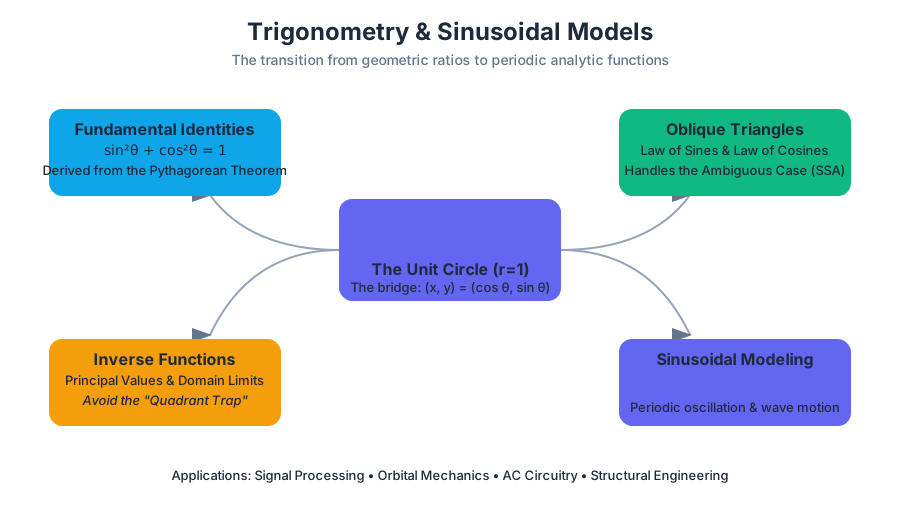
Trigonometry is often introduced as the study of right-angled triangles, but in advanced mathematics and engineering, it evolves into the study of circular functions and periodic phenomena. While a triangle is static, a circle represents rotation, and rotation over time yields a wave. This section explores the transition from geometric ratios to analytic functions, providing the toolkit necessary to model everything from the orbit of planets to the oscillation of an alternating current (AC) circuit.
The Unit Circle and Fundamental Identities
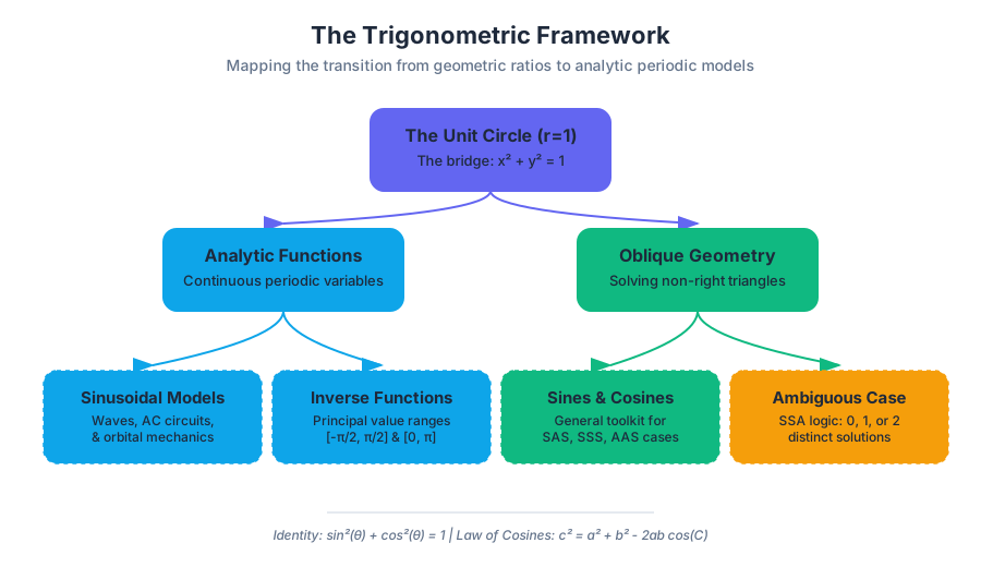
The Unit Circle is a circle with a radius of $r = 1$ centered at the origin $(0,0)$ of the Cartesian plane. It serves as the bridge between geometry and algebra. For any angle $\theta$ in standard position, the terminal side intersects the unit circle at a point $P(x, y)$.
What it is
The coordinates of $P$ are defined as:
- $x = \cos(\theta)$
- $y = \sin(\theta)$
Because the equation of the unit circle is $x^2 + y^2 = 1$, we derive the Pythagorean Identity: $$\sin^2(\theta) + \cos^2(\theta) = 1$$
Why it matters
The unit circle allows us to extend trigonometric functions beyond $90^\circ$. It defines the functions for all real numbers, creating the foundation for calculus (where $\theta$ is treated as a continuous variable in radians) and signal processing.
How it works: Special Values
The symmetry of the unit circle allows us to determine exact values for common angles ($30^\circ, 45^\circ, 60^\circ$) across all four quadrants.
| Angle (Deg) | Angle (Rad) | $\sin(\theta)$ | $\cos(\theta)$ | $\tan(\theta)$ |
|---|---|---|---|---|
| $0^\circ$ | $0$ | $0$ | $1$ | $0$ |
| $30^\circ$ | $\pi/6$ | $1/2$ | $\sqrt{3}/2$ | $\sqrt{3}/3$ |
| $45^\circ$ | $\pi/4$ | $\sqrt{2}/2$ | $\sqrt{2}/2$ | $1$ |
| $60^\circ$ | $\pi/3$ | $\sqrt{3}/2$ | $1/2$ | $\sqrt{3}$ |
| $90^\circ$ | $\pi/2$ | $1$ | $0$ | Undefined |
Implementation: Coordinate Mapping
In computational geometry, we frequently convert polar coordinates (angle and distance) to Cartesian coordinates (x and y).
import numpy as np

def polar_to_cartesian(radius, theta_degrees):
    """
    Converts polar coordinates to Cartesian coordinates using NumPy.
    Demonstrates the fundamental application of unit circle logic.
    """
    # Convert degrees to radians: radians = degrees * (pi / 180)
    theta_radians = np.radians(theta_degrees)

    # x = r * cos(theta), y = r * sin(theta)
    x = radius * np.cos(theta_radians)
    y = radius * np.sin(theta_radians)

    return x, y

# Example: A point 5 units away at a 120-degree angle
point = polar_to_cartesian(5, 120)
print(f"Coordinates: x={point[0]:.2f}, y={point[1]:.2f}")
# Output: Coordinates: x=-2.50, y=4.33
Inverse Trigonometric Functions and Domain Restrictions
To "undo" a trigonometric function, we use inverse functions: $\arcsin(x)$, $\arccos(x)$, and $\arctan(x)$. However, because trigonometric functions are periodic, they are not one-to-one. A single $y$-value (like $0.5$) corresponds to infinitely many $x$-values (angles).
What it is
To create a true inverse function, we must restrict the domain of the original function so that it passes the horizontal line test.
Definition: Principal Values The range of an inverse trigonometric function is restricted to a specific set of "principal values" to ensure a unique output for every input.
| Function | Notation | Domain | Range (Principal Interval) |
|---|---|---|---|
| Inverse Sine | $\sin^{-1}(x)$ | $[-1, 1]$ | $[-\pi/2, \pi/2]$ |
| Inverse Cosine | $\cos^{-1}(x)$ | $[-1, 1]$ | $[0, \pi]$ |
| Inverse Tangent | $\tan^{-1}(x)$ | $(-\infty, \infty)$ | $(-\pi/2, \pi/2)$ |
Common Pitfalls: The Quadrant Trap
A common error is assuming $\sin^{-1}(\sin(\theta)) = \theta$ for all $\theta$. This is only true if $\theta$ is within the restricted range. For example, $\sin^{-1}(\sin(150^\circ)) = 30^\circ$, because $30^\circ$ is the principal value in the allowed range that shares the same sine value as $150^\circ$.
General Triangles: Law of Sines and Law of Cosines
While basic trig handles right triangles, the Law of Sines and Law of Cosines allow us to solve for any triangle (oblique triangles).
Law of Sines
Used when we know a side and its opposite angle. $$\frac{a}{\sin A} = \frac{b}{\sin B} = \frac{c}{\sin C}$$
Law of Cosines
A generalization of the Pythagorean theorem, used when we have two sides and the included angle (SAS) or three sides (SSS). $$c^2 = a^2 + b^2 - 2ab \cos(C)$$
Mathematical Derivation: Law of Cosines
The Law of Cosines can be derived by placing a triangle on the Cartesian plane and using the distance formula.
\text{Let vertex } C \text{ be at } (0,0).
\text{Then vertex } A \text{ is at } (b, 0) \text{ and vertex } B \text{ is at } (a \cos C, a \sin C).
\text{The distance } c \text{ between } A \text{ and } B \text{ is:}
c^2 = (a \cos C - b)^2 + (a \sin C - 0)^2
c^2 = a^2 \cos^2 C - 2ab \cos C + b^2 + a^2 \sin^2 C
c^2 = a^2(\cos^2 C + \sin^2 C) + b^2 - 2ab \cos C
\text{Since } \cos^2 C + \sin^2 C = 1:
c^2 = a^2 + b^2 - 2ab \cos C
The Ambiguous Case (SSA)
When using the Law of Sines with two sides and a non-included angle (Side-Side-Angle), three possibilities exist:
- No triangle exists (the side is too short to reach).
- Exactly one triangle exists (a right triangle or only one possible orientation).
- Two distinct triangles exist (the "swinging door" effect where the side can hinge inward or outward).
| Condition ($a, b, A$) | Number of Triangles |
|---|---|
| $a < b \sin A$ | 0 |
| $a = b \sin A$ | 1 (Right Triangle) |
| $b \sin A < a < b$ | 2 (Ambiguous Case) |
| $a \ge b$ | 1 |
Sinusoidal Modeling
A sinusoid is a mathematical curve that describes a smooth periodic oscillation. It is the most efficient way to model repetitive data.
The Standard Equation
The general form of a sinusoidal function is: $$y = A \sin(B(x - C)) + D$$
Where:
- $A$ (Amplitude): The vertical stretch; half the distance between the maximum and minimum values.
- $P$ (Period): The horizontal length of one full cycle. $P = \frac{2\pi}{|B|}$.
- $C$ (Phase Shift): The horizontal displacement.
- $D$ (Vertical Shift/Midline): The average value of the function.
Real-World Usage: Audio Synthesis
In digital music, a "pure tone" is a simple sine wave. By modulating the frequency and amplitude, we can synthesize sounds.
// Web Audio API Example: Generating a Sinusoidal Tone
const audioCtx = new (window.AudioContext || window.webkitAudioContext)();

function playTone(frequency, duration) {
    const oscillator = audioCtx.createOscillator();
    const gainNode = audioCtx.createGain();

    // The 'sine' type is a pure sinusoidal model
    oscillator.type = 'sine';
    oscillator.frequency.setValueAtTime(frequency, audioCtx.currentTime);

    // Amplitude control (Volume)
    gainNode.gain.setValueAtTime(0.5, audioCtx.currentTime);
    gainNode.gain.exponentialRampToValueAtTime(0.0001, audioCtx.currentTime + duration);

    oscillator.connect(gainNode);
    gainNode.connect(audioCtx.destination);

    oscillator.start();
    oscillator.stop(audioCtx.currentTime + duration);
}

// Play a 440Hz (Middle A) tone for 2 seconds
// playTone(440, 2);
Modeling Workflow
To model real-world data (e.g., temperature over a year):
- Identify Midline ($D$): Calculate $\frac{\text{max} + \text{min}}{2}$.
- Identify Amplitude ($A$): Calculate $\text{max} - D$.
- Identify Period ($P$): Determine the time for one cycle (e.g., 12 months) and solve for $B = \frac{2\pi}{P}$.
- Identify Phase Shift ($C$): Find where the data starts its upward trend relative to a standard sine wave starting at the midline.
Angle Addition and Composite Identities
In many engineering applications, we need to decompose a complex wave into simpler components or rotate a vector by a specific angle. This is where Angle Addition Identities become essential.
The Core Identities
Sum and Difference Formulas
- $\sin(\alpha \pm \beta) = \sin \alpha \cos \beta \pm \cos \alpha \sin \beta$
- $\cos(\alpha \pm \beta) = \cos \alpha \cos \beta \mp \sin \alpha \sin \beta$
- $\tan(\alpha \pm \beta) = \frac{\tan \alpha \pm \tan \beta}{1 \mp \tan \alpha \tan \beta}$
Double-Angle Identities
Derived by setting $\alpha = \beta = \theta$:
- $\sin(2\theta) = 2 \sin \theta \cos \theta$
- $\cos(2\theta) = \cos^2 \theta - \sin^2 \theta = 2\cos^2 \theta - 1 = 1 - 2\sin^2 \theta$
Performance Implementation: Fixed-Point Trigonometry
In embedded systems (like a microwave controller or a simple drone), calculating sin() using floating-point math is too slow. Engineers use Lookup Tables (LUT) and identities to save cycles.
#include <stdio.h>

// Precomputed sine values for 0-90 degrees, scaled by 256 (8-bit fixed point)
const int SIN_LUT[] = {0, 4, 8, 13, 17, 22, 26, 31, 35, 40, 44, 48, 53, 57, 61, 65, 70, 74, 78, 83, 87, 91, 95, 99, 103, 107, 111, 115, 119, 123, 127, 131, 135, 138, 142, 146, 149, 153, 156, 160, 163, 167, 170, 173, 177, 180, 183, 186, 189, 192, 195, 198, 201, 204, 206, 209, 211, 214, 216, 219, 221, 223, 225, 227, 229, 231, 233, 235, 236, 238, 240, 241, 243, 244, 245, 246, 247, 248, 249, 250, 251, 252, 253, 253, 254, 254, 255, 255, 255, 255, 256};

int fast_sin(int degrees) {
    // Normalize angle to 0-359
    degrees = degrees % 360;
    if (degrees < 0) degrees += 360;

    // Use symmetry to calculate sin for all quadrants
    if (degrees <= 90) return SIN_LUT[degrees];
    if (degrees <= 180) return SIN_LUT[180 - degrees];
    if (degrees <= 270) return -SIN_LUT[degrees - 180];
    return -SIN_LUT[360 - degrees];
}

int main() {
    printf("Fixed-point sin(210): %d/256\n", fast_sin(210));
    // Output: -127/256 (approx -0.496, very close to -0.5)
    return 0;
}
Summary of Sinusoidal Parameters
When analyzing a waveform, the following table serves as a quick reference for relating the algebraic equation to the physical graph.
| Parameter | Algebraic Role | Graphical Effect | Physical Analogy |
|---|---|---|---|
| $A$ | Coefficient of Sine | Vertical Stretch | Volume / Brightness |
| $B$ | Frequency Factor | Horizontal Compression | Pitch / Color (Frequency) |
| $C$ | Horizontal Shift | Lateral Translation | Delay / Timing |
| $D$ | Constant Term | Vertical Translation | DC Offset / Baseline |
Advanced Applications: Fourier Analysis
While this unit focuses on single sinusoids, it is important to note that any periodic function (square waves, sawtooth waves, or human speech) can be represented as a sum of infinite sine and cosine waves. This is known as a Fourier Series. The identities learned here (specifically angle addition and product-to-sum) are the mechanics that allow us to decompose these complex signals into their constituent frequencies.
Complex Numbers and Polar Form
Key concepts: Complex plane · Polar coordinates · De Moivre's Theorem · Magnitude and argument
Explores the representation of complex numbers in the complex plane and the conversion between rectangular and polar forms.
Complex Numbers and Polar Form
The transition from the real number line to the complex plane represents one of the most significant leaps in mathematical history. While real numbers allow us to measure magnitude along a single dimension, complex numbers introduce the concept of phase and rotation, providing a two-dimensional framework for algebra. In this deep dive, we move beyond the basic definition of the imaginary unit $i = \sqrt{-1}$ to explore the Polar Form of complex numbers—a representation that transforms difficult algebraic expansions into simple geometric rotations.
The Geometry of the Complex Plane
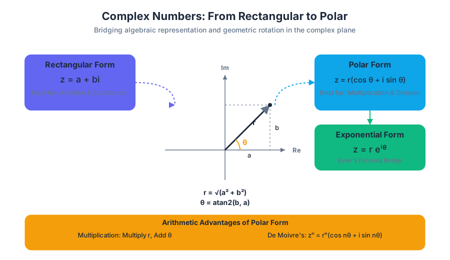
To understand polar form, we must first master the environment in which complex numbers live: the Complex Plane (or Argand Diagram). Unlike the standard Cartesian plane where $x$ and $y$ represent two independent physical dimensions, the complex plane treats the horizontal axis as the Real axis ($\text{Re}$) and the vertical axis as the Imaginary axis ($\text{Im}$).
A complex number $z = a + bi$ is represented as a point $(a, b)$ or a vector originating from the origin to that point.
The Modulus and Argument
Every point in the complex plane can be uniquely identified by its distance from the origin and its angle relative to the positive real axis.
- Modulus ($r$ or $|z|$): The non-negative distance from the origin to the point $a + bi$. By the Pythagorean theorem, $r = \sqrt{a^2 + b^2}$.
- Argument ($\theta$ or $\arg(z)$): The angle formed with the positive real axis, typically measured in radians. It is calculated using the arctangent function, though care must be taken regarding the quadrant: $\theta = \operatorname{atan2}(b, a)$.
Definition: The Principal Argument While any angle $\theta + 2\pi k$ (for integer $k$) identifies the same point, the Principal Argument $\operatorname{Arg}(z)$ is restricted to the interval $(-\pi, \pi]$ or $[0, 2\pi)$.
| Property | Rectangular Form ($a + bi$) | Polar Form ($r(\cos \theta + i \sin \theta)$) |
|---|---|---|
| Primary Use | Addition and Subtraction | Multiplication, Division, and Powers |
| Components | Real part ($a$) and Imaginary part ($b$) | Magnitude ($r$) and Phase ($\theta$) |
| Visual Logic | Grid-based displacement | Vector length and rotation |
| Zero Value | $0 + 0i$ | $r = 0$, $\theta$ is undefined |
Conversion Mechanics: Rectangular to Polar
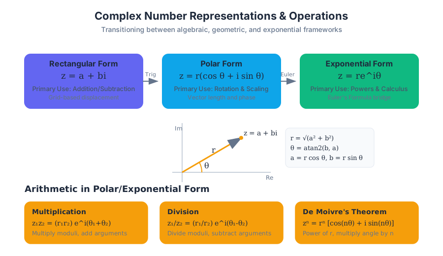
The bridge between the rectangular and polar worlds is built on basic trigonometry. If we treat the modulus $r$ as the hypotenuse of a right triangle, the legs are $a = r \cos \theta$ and $b = r \sin \theta$.
The Polar Representation
Substituting these into $z = a + bi$ gives: $$z = r \cos \theta + i(r \sin \theta) = r(\cos \theta + i \sin \theta)$$ This is often abbreviated as $r \operatorname{cis} \theta$.
Worked Example: Converting $z = -1 + i\sqrt{3}$
- Find $r$: $r = \sqrt{(-1)^2 + (\sqrt{3})^2} = \sqrt{1 + 3} = 2$.
- Find $\theta$: The point $(-1, \sqrt{3})$ lies in the second quadrant. $$\tan \theta = \frac{\sqrt{3}}{-1} = -\sqrt{3}$$ The reference angle is $\pi/3$. In the second quadrant, $\theta = \pi - \pi/3 = 2\pi/3$.
- Result: $z = 2(\cos \frac{2\pi}{3} + i \sin \frac{2\pi}{3})$.
import cmath
import math

def analyze_complex_number(a, b):
    """
    Performs a deep analysis of a complex number z = a + bi,
    converting it to polar form and calculating its properties.
    """
    z = complex(a, b)

    # Magnitude (Modulus)
    r = abs(z)

    # Phase (Argument) in radians
    theta = cmath.phase(z)

    # Convert phase to degrees for readability
    theta_deg = math.degrees(theta)

    return {
        "rectangular": f"{a} + {b}j",
        "modulus": r,
        "argument_rad": theta,
        "argument_deg": theta_deg,
        "polar_string": f"{r:.2f} * (cos({theta:.2f}) + i*sin({theta:.2f}))"
    }

# Example: z = -1 + sqrt(3)i
print(analyze_complex_number(-1, math.sqrt(3)))
Euler’s Formula: The Exponential Bridge
The most profound realization in complex analysis is Euler's Formula, which links trigonometric functions to the natural exponential function: $$e^{i\theta} = \cos \theta + i \sin \theta$$ This allows us to write complex numbers in Exponential Form: $z = re^{i\theta}$. This is not merely a shorthand; it reveals that complex multiplication is governed by the laws of exponents.
Arithmetic in Polar Form
While adding complex numbers in rectangular form is trivial ($(a+bi) + (c+di) = (a+c) + (b+d)i$), multiplication and division are cumbersome. In polar form, these operations become elegant.
Multiplication
To multiply two complex numbers, multiply their moduli and add their arguments: $$z_1 z_2 = (r_1 e^{i\theta_1})(r_2 e^{i\theta_2}) = r_1 r_2 e^{i(\theta_1 + \theta_2)}$$
Division
To divide two complex numbers, divide their moduli and subtract their arguments: $$\frac{z_1}{z_2} = \frac{r_1}{r_2} e^{i(\theta_1 - \theta_2)}$$
| Operation | Rectangular Complexity | Polar Complexity | Geometric Interpretation |
|---|---|---|---|
| Multiplication | High (FOIL + $i^2$ simplification) | Low (Scalar mult + Addition) | Scaling and Rotation |
| Division | High (Conjugate multiplication) | Low (Scalar div + Subtraction) | Inverse Scaling and Rotation |
| Powers | Extremely High (Binomial expansion) | Negligible (De Moivre's) | Repeated Rotation |
De Moivre’s Theorem
When we raise a complex number to an integer power $n$, the polar form yields a powerful shortcut known as De Moivre's Theorem: $$z^n = [r(\cos \theta + i \sin \theta)]^n = r^n(\cos n\theta + i \sin n\theta)$$
Derivation via Euler's Formula
The proof becomes trivial when using the exponential form: $$(re^{i\theta})^n = r^n (e^{i\theta})^n = r^n e^{i(n\theta)}$$ Converting back to trigonometric form: $$r^n (\cos(n\theta) + i \sin(n\theta))$$
\begin{aligned}
\text{Problem: Calculate } (1+i)^8 \\
\text{1. Convert to Polar: } & r = \sqrt{1^2+1^2} = \sqrt{2}, \theta = \pi/4 \\
& z = \sqrt{2} e^{i\pi/4} \\
\text{2. Apply De Moivre's: } & z^8 = (\sqrt{2})^8 e^{i(8 \cdot \pi/4)} \\
& z^8 = 2^4 e^{i(2\pi)} \\
\text{3. Simplify: } & 16(\cos 2\pi + i \sin 2\pi) \\
& 16(1 + 0i) = 16
\end{aligned}
Finding Complex Roots (Roots of Unity)
One of the most important applications of polar form is solving equations of the form $z^n = w$. Unlike real numbers, where a number might have only one or two real roots, every non-zero complex number has exactly $n$ distinct $n$-th roots.
To find the $n$-th roots of $w = R(\cos \phi + i \sin \phi)$:
- Take the $n$-th root of the modulus: $r = \sqrt[n]{R}$.
- Divide the argument by $n$ and add increments of $2\pi/n$: $$\theta_k = \frac{\phi + 2\pi k}{n} \quad \text{for } k = 0, 1, 2, \dots, n-1$$
The $n$-th Roots of Unity
The roots of $z^n = 1$ are called the Roots of Unity. Geometrically, they form a regular $n$-gon inscribed in the unit circle, with one vertex at $(1, 0)$.
| $n$ | Equation | Roots (Exponential Form) | Geometric Shape |
|---|---|---|---|
| 2 | $z^2 = 1$ | $e^{i0}, e^{i\pi}$ | Line segment (1, -1) |
| 3 | $z^3 = 1$ | $e^{i0}, e^{i2\pi/3}, e^{i4\pi/3}$ | Equilateral Triangle |
| 4 | $z^4 = 1$ | $e^{i0}, e^{i\pi/2}, e^{i\pi}, e^{i3\pi/2}$ | Square |
| 6 | $z^6 = 1$ | $e^{i2\pi k/6}$ for $k \in {0..5}$ | Regular Hexagon |
Real-World Application: Phasors and AC Circuits
In electrical engineering, alternating current (AC) signals are sinusoidal. Analyzing circuits with resistors, capacitors, and inductors using differential equations is difficult. Instead, engineers use Phasors—complex numbers in polar form that represent the amplitude and phase of the sine wave.
- Voltage: $V(t) = V_{peak} \cos(\omega t + \phi)$ is represented as $V_{peak} \angle \phi$.
- Impedance ($Z$): Resistors have real impedance ($R$), while capacitors and inductors have imaginary impedance ($jX$).
- Ohm's Law for AC: $V = I \cdot Z$. Because these are complex numbers, this single equation handles both the change in magnitude and the shift in phase simultaneously.
/**
 * Example: Calculating Total Impedance in an AC Circuit
 * Z_total = Z_resistor + Z_inductor + Z_capacitor
 * In polar form, this allows us to see the phase shift of the current.
 */

class Complex {
    constructor(re, im) {
        this.re = re;
        this.im = im;
    }

    add(other) {
        return new Complex(this.re + other.re, this.im + other.im);
    }

    getMagnitude() {
        return Math.sqrt(this.re**2 + this.im**2);
    }

    getAngle() {
        return Math.atan2(this.im, this.re) * (180 / Math.PI);
    }

    toPolarString() {
        return `${this.getMagnitude().toFixed(2)} ∠ ${this.getAngle().toFixed(2)}°`;
    }
}

// Circuit: 100 Ohm resistor, 50j Ohm inductor (inductive reactance)
const R = new Complex(100, 0);
const L = new Complex(0, 50);
const Z_total = R.add(L);

console.log(`Total Impedance: ${Z_total.toPolarString()}`);
// Output: Total Impedance: 111.80 ∠ 26.57°
Common Pitfalls and Edge Cases
- The
atanTrap: When converting to polar form, the simple formula $\theta = \arctan(b/a)$ only works for the first and fourth quadrants ($a > 0$). If $a < 0$, you must add $\pi$ (or 180°) to the result to reach the correct quadrant. - The Zero Modulus: The number $0 + 0i$ has a modulus of 0, but its argument is undefined. In polar form, the origin is a singularity.
- Degree vs. Radian Confusion: Most theoretical mathematics (and De Moivre's Theorem) assumes radians. Using degrees inside $e^{i\theta}$ is a common notation error in physics that can lead to calculation failures in software.
- Multi-valued Roots: Forgetting that there are $n$ roots for $z^n = w$. Students often find the "principal" root and ignore the other $n-1$ rotations.
Summary Table: Domain Mapping
| Field | Usage of Polar Form | Key Benefit |
|---|---|---|
| Quantum Mechanics | Wavefunctions ($\psi$) | Probability amplitudes are complex; phase represents interference. |
| Signal Processing | Fourier Transforms | Decomposes signals into frequency components (magnitude/phase). |
| Control Theory | Stability Analysis | Poles and zeros in the complex plane determine system oscillation. |
| Computer Graphics | 2D Rotations | Multiplying by $e^{i\theta}$ rotates a point without matrix math. |
Rational Functions
Key concepts: Vertical and horizontal asymptotes · Removable discontinuities (holes) · End behavior · Rational expression arithmetic
Analysis of functions defined as quotients of polynomials, focusing on their graphical behavior and discontinuities.
Rational Functions
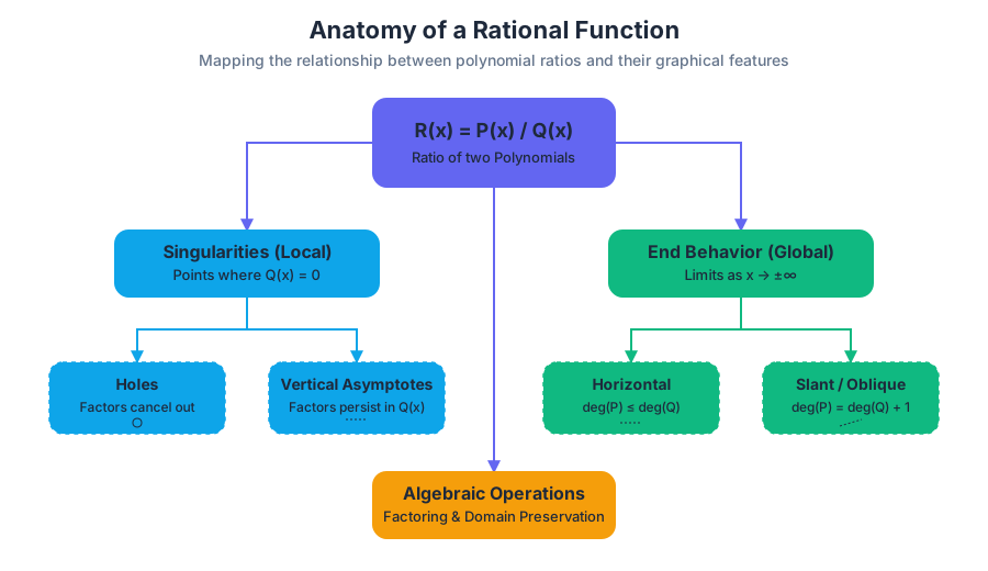
Rational functions represent the ratio of two polynomial expressions. In the landscape of algebraic structures, they serve as the bridge between simple polynomial behavior and the complex world of transcendental functions. While a polynomial is defined for all real numbers and exhibits relatively predictable end behavior, a rational function is defined by its singularities—the points where the function "breaks" or heads toward infinity.
Formally, a rational function $R(x)$ is defined as:
Definition: $R(x) = \frac{P(x)}{Q(x)}$, where $P(x)$ and $Q(x)$ are polynomial functions and $Q(x) \neq 0$.
The domain of $R(x)$ is the set of all real numbers except for the roots of the denominator $Q(x)$. These excluded values are the architects of the function's most interesting features: vertical asymptotes and removable discontinuities.
Arithmetic of Rational Expressions
Before analyzing the calculus-like behavior of these functions, one must master the algebraic manipulation of the underlying expressions. Arithmetic with rational expressions mirrors arithmetic with fractions, requiring a common denominator for addition and subtraction, and prime factorization (in this case, polynomial factoring) for simplification.
Simplification and Domain Preservation
To simplify a rational expression, we factor both the numerator and denominator and cancel common factors. However, a critical "memory" of the original function must be maintained. If a factor $(x - c)$ is canceled, the value $x = c$ is still excluded from the domain of the original function, even if the simplified version appears defined there.
| Operation | Procedure | Key Requirement |
|---|---|---|
| Multiplication | $\frac{A}{B} \cdot \frac{C}{D} = \frac{AC}{BD}$ | Factor first to cancel common terms across numerators/denominators. |
| Division | $\frac{A}{B} \div \frac{C}{D} = \frac{A}{B} \cdot \frac{D}{C}$ | Multiply by the reciprocal; check domain for both $C$ and $D$. |
| Addition | $\frac{A}{B} + \frac{C}{D} = \frac{AD + BC}{BD}$ | Find the Least Common Multiple (LCM) of the denominators. |
| Simplification | $\frac{k \cdot P(x)}{k \cdot Q(x)} = \frac{P(x)}{Q(x)}$ | $k$ must be a non-zero polynomial factor. |
Implementation: Symbolic Manipulation
In computational mathematics, we often use symbolic engines to handle these reductions to ensure precision and track domain restrictions.
import sympy as sp

def analyze_rational_expression(num_expr, den_expr):
    """
    Analyzes a rational function using symbolic math.
    Returns the simplified form and the points of discontinuity.
    """
    x = sp.symbols('x')
    P = sp.poly(num_expr, x)
    Q = sp.poly(den_expr, x)

    # Original rational function
    R = P / Q

    # Identify domain restrictions (roots of denominator)
    domain_restrictions = sp.solve(Q, x)

    # Simplify (cancels common factors)
    R_simplified = sp.simplify(R)

    # Identify holes vs asymptotes
    holes = []
    asymptotes = []

    for root in domain_restrictions:
        # If the limit exists and is finite, it's a hole
        limit_val = sp.limit(R, x, root)
        if limit_val.is_finite:
            holes.append(root)
        else:
            asymptotes.append(root)

    return {
        "simplified": R_simplified,
        "holes": holes,
        "vertical_asymptotes": asymptotes
    }

# Example: (x^2 - 1) / (x^2 - x)
# Factors to: (x-1)(x+1) / x(x-1)
# Result: (x+1)/x with a hole at x=1
print(analyze_rational_expression("x**2 - 1", "x**2 - x"))
Discontinuities: Holes vs. Asymptotes
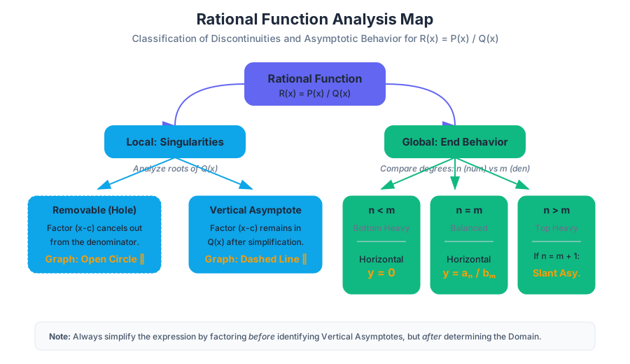
The most fundamental task in analyzing a rational function is determining what happens at the values of $x$ where $Q(x) = 0$. These points of undefined behavior fall into two distinct categories: Removable Discontinuities and Non-removable Discontinuities.
Removable Discontinuities (Holes)
A hole occurs at $x = c$ if the factor $(x - c)$ exists in both the numerator and the denominator. When you evaluate the limit of the function as $x$ approaches $c$, the result is a finite number, even though the function itself is undefined at that exact point.
Non-removable Discontinuities (Vertical Asymptotes)
A vertical asymptote occurs at $x = c$ if, after simplifying the expression, the factor $(x - c)$ remains in the denominator. As $x$ approaches $c$, the function's output grows without bound ($+\infty$ or $-\infty$).
| Feature | Mathematical Condition | Graphical Representation |
|---|---|---|
| Hole | $(x-c)$ is a factor of both $P(x)$ and $Q(x)$ with equal or greater multiplicity in $P(x)$. | An open circle at $(c, L)$, where $L$ is the limit. |
| Vertical Asymptote | $(x-c)$ is a factor of $Q(x)$ after all common factors are canceled. | A vertical dashed line $x=c$ that the graph never crosses. |
End Behavior and Horizontal Asymptotes
While vertical asymptotes describe "local" behavior near specific points, Horizontal Asymptotes describe the "global" or End Behavior of the function as $x \to \infty$ or $x \to -\infty$. This behavior is determined entirely by the degrees of the numerator ($n$) and the denominator ($m$).
The Degree Comparison Rule
Let $P(x) = a_n x^n + \dots$ and $Q(x) = b_m x^m + \dots$.
- If $n < m$: The denominator grows faster than the numerator. The horizontal asymptote is the x-axis: $y = 0$.
- If $n = m$: The numerator and denominator grow at the same rate. The horizontal asymptote is the ratio of the leading coefficients: $y = \frac{a_n}{b_m}$.
- If $n > m$: The numerator grows faster. There is no horizontal asymptote.
- If $n = m + 1$, there is a Slant (Oblique) Asymptote, found via polynomial long division.
- If $n > m + 1$, the end behavior follows the power function $x^{n-m}$.
Formal Derivation via Limits
To prove the $n=m$ case, we divide every term in the expression by $x^n$ (the highest power).
\lim_{x \to \infty} \frac{a_n x^n + a_{n-1} x^{n-1} + \dots}{b_n x^n + b_{n-1} x^{n-1} + \dots}
= \lim_{x \to \infty} \frac{a_n + \frac{a_{n-1}}{x} + \dots}{b_n + \frac{b_{n-1}}{x} + \dots}
= \frac{a_n + 0 + \dots}{b_n + 0 + \dots}
= \frac{a_n}{b_n}
This derivation highlights why lower-degree terms become irrelevant at extreme values of $x$: they vanish as their denominators grow.
Oblique (Slant) Asymptotes
When the degree of the numerator is exactly one higher than the degree of the denominator, the function does not settle into a horizontal line; instead, it approaches a linear path.
Theorem: If $R(x) = \frac{P(x)}{Q(x)}$ and $\text{deg}(P) = \text{deg}(Q) + 1$, then $R(x)$ can be written as $R(x) = (mx + b) + \frac{r(x)}{Q(x)}$, where $mx + b$ is the quotient and $r(x)$ is the remainder. As $x \to \infty$, $\frac{r(x)}{Q(x)} \to 0$, and the graph approaches the line $y = mx + b$.
Worked Example: Finding a Slant Asymptote
Consider $f(x) = \frac{x^2 + 3x + 2}{x - 1}$.
- Perform Long Division: Divide $x^2 + 3x + 2$ by $x - 1$.
- Quotient: $x + 4$.
- Remainder: $6$.
- Result: $f(x) = x + 4 + \frac{6}{x - 1}$.
- Asymptote: As $x \to \infty$, the term $\frac{6}{x-1}$ vanishes. The slant asymptote is $y = x + 4$.
Graphing Rational Functions: A Systematic Pipeline
Graphing a rational function manually requires synthesizing all the concepts discussed. A senior mathematician follows a specific "pipeline" to ensure no features are missed.
- Factor Everything: Completely factor $P(x)$ and $Q(x)$.
- Find Intercepts:
- y-intercept: Set $x=0$.
- x-intercepts (Zeros): Set the simplified numerator to zero.
- Identify Discontinuities:
- Find roots of $Q(x)$.
- Classify as holes or vertical asymptotes.
- Determine End Behavior: Compare degrees to find horizontal or slant asymptotes.
- Sign Analysis (Test Points): Use the zeros and vertical asymptotes to divide the x-axis into intervals. Determine if the function is positive or negative in each interval.
- Check for Asymptote Crossing: Unlike vertical asymptotes, a function can cross a horizontal asymptote. Solve $R(x) = \text{Asymptote Value}$ to check.
Real-World Usage Example: Concentration Modeling
In chemical engineering, rational functions model the concentration of a solute in a mixture over time.
/**
 * Models the concentration of salt in a tank.
 * C(t) = (InitialSalt + RateIn * ConcentrationIn * t) / (InitialVolume + NetFlowRate * t)
 */
interface TankParams {
    initialSalt: number;      // grams
    initialVolume: number;    // liters
    saltInflowRate: number;   // grams/minute
    volumeInflowRate: number; // liters/minute
}

function getConcentrationAtTime(t: number, params: TankParams): number {
    const numerator = params.initialSalt + (params.saltInflowRate * t);
    const denominator = params.initialVolume + (params.volumeInflowRate * t);

    if (denominator === 0) {
        throw new Error("Singularity: Tank is empty.");
    }

    return numerator / denominator;
}

// As t -> infinity, the concentration approaches (saltInflowRate / volumeInflowRate)
// This is the horizontal asymptote of the rational function.
const myTank: TankParams = {
    initialSalt: 100,
    initialVolume: 1000,
    saltInflowRate: 20,
    volumeInflowRate: 5
};

console.log(`Concentration at 100 mins: ${getConcentrationAtTime(100, myTank)} g/L`);
console.log(`Steady state (Asymptote): ${myTank.saltInflowRate / myTank.volumeInflowRate} g/L`);
Common Pitfalls and Edge Cases
Even experienced students stumble on the nuances of rational functions.
- The "Hole" Displacement: Forgetting that a hole has a y-coordinate. To find it, plug the x-value of the hole into the simplified function.
- Crossing Asymptotes: Believing that a graph can never cross a horizontal asymptote. Horizontal asymptotes only describe behavior at the ends of the graph; the function can cross them many times in the middle.
- Multiplicity at Asymptotes: If a vertical asymptote factor $(x-c)$ has an even multiplicity (e.g., $1/(x-c)^2$), the graph goes to the same infinity on both sides (a "volcano" shape). If it's odd, they go to opposite infinities.
- Domain of the Inverse: When finding the inverse of a rational function, the horizontal asymptote of the original becomes the vertical asymptote (domain restriction) of the inverse.
| Pitfall | Correction |
|---|---|
| Ignoring Holes | Always factor and simplify before identifying vertical asymptotes. |
| Misidentifying Slant Asymptotes | Only exists if $\text{deg}(Num) = \text{deg}(Den) + 1$. |
| Incorrect Sign Analysis | Signs only change at zeros or vertical asymptotes with odd multiplicity. |
Extensions: Partial Fraction Decomposition
In Calculus, specifically for integration, we often need to reverse the process of adding rational expressions. This is called Partial Fraction Decomposition (PFD). It allows us to break a complex rational function into a sum of simpler "partial" fractions.
For example: $$\frac{5x - 1}{(x - 3)(x + 2)} = \frac{A}{x - 3} + \frac{B}{x + 2}$$
By solving for $A$ and $B$, we transform a product-based denominator into a sum of simple linear denominators, which are significantly easier to integrate or transform using Laplace methods. This highlights the "Why it matters" aspect: rational functions are the building blocks for solving differential equations in engineering.
Conic Sections
Key concepts: Standard equations of ellipses · Standard equations of hyperbolas · Foci, vertices, and centers · Planetary motion applications
Study of the geometric and algebraic properties of ellipses and hyperbolas, including their standard equations and real-world applications.
Conic Sections
Conic sections represent the locus of points formed by the intersection of a plane and a right circular double cone. While the circle and parabola are fundamental members of this family, the ellipse and the hyperbola represent the most mathematically rich and physically significant structures in the group. From the celestial mechanics governing the motion of planets to the hyperbolic trajectories of non-returning comets and the design of sophisticated cooling towers, these curves provide the geometric language for the physical universe.
In this deep dive, we will move beyond basic recognition of shapes to explore the rigorous algebraic derivations, the relationship between focal points and vertices, and the practical implementation of these curves in computational models.
The Geometric Foundation: Slicing the Cone
The nature of a conic section is determined by the angle at which the plane intersects the cone relative to the cone's slant height.
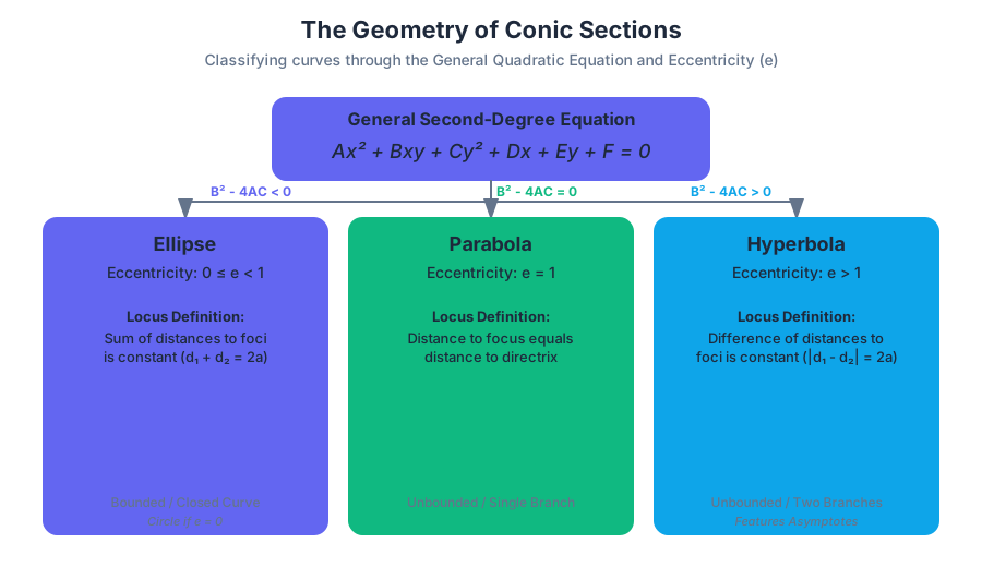
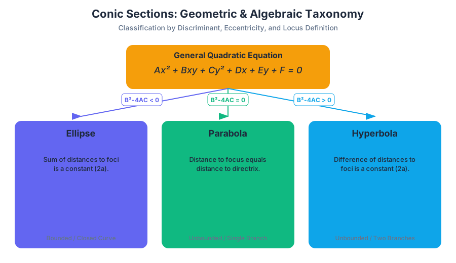
Definition: The General Quadratic Equation Every conic section can be represented by the general second-degree equation in two variables: $$Ax^2 + Bxy + Cy^2 + Dx + Ey + F = 0$$ The discriminant ($B^2 - 4AC$) determines the type of curve:
- If $B^2 - 4AC < 0$, the curve is an ellipse (or a circle if $A=C$ and $B=0$).
- If $B^2 - 4AC > 0$, the curve is a hyperbola.
- If $B^2 - 4AC = 0$, the curve is a parabola.
Comparison of Conic Properties
| Property | Ellipse | Hyperbola | Parabola |
|---|---|---|---|
| Eccentricity ($e$) | $0 \le e < 1$ | $e > 1$ | $e = 1$ |
| Locus Definition | Sum of distances to foci is constant ($d_1 + d_2 = 2a$) | Difference of distances to foci is constant ($ | d_1 - d_2 |
| Boundedness | Bounded (Closed curve) | Unbounded (Two branches) | Unbounded (One branch) |
| Major Features | Two foci, two vertices, center | Two foci, two vertices, center, two asymptotes | One focus, one vertex, directrix |
The Ellipse: The Closed Curve of Sums
An ellipse is the set of all points $(x, y)$ in a plane such that the sum of the distances from two fixed points (the foci) is a constant, denoted as $2a$. This constant $2a$ is also the length of the major axis.
Standard Equations and Orientation
The orientation of an ellipse depends on which denominator is larger. We define $a$ as the semi-major axis and $b$ as the semi-minor axis, where $a > b$.
| Orientation | Standard Equation (Center $(h, k)$) | Foci Locations | Vertices |
|---|---|---|---|
| Horizontal | $\frac{(x-h)^2}{a^2} + \frac{(y-k)^2}{b^2} = 1$ | $(h \pm c, k)$ | $(h \pm a, k)$ |
| Vertical | $\frac{(x-h)^2}{b^2} + \frac{(y-k)^2}{a^2} = 1$ | $(h, k \pm c)$ | $(h, k \pm a)$ |
The Pythagorean Relationship
In an ellipse, the distance from the center to each focus is $c$. These values are related by the equation: $$c^2 = a^2 - b^2$$ This relationship is intuitive if one considers a point at the end of the minor axis. The distance from that point to either focus is exactly $a$, forming a right triangle with legs $b$ and $c$ and hypotenuse $a$.
Derivation of the Standard Form
To understand why the equation takes this form, consider an ellipse centered at $(0,0)$ with foci at $(-c, 0)$ and $(c, 0)$. Let $P(x, y)$ be a point on the ellipse. By definition: $$\sqrt{(x+c)^2 + y^2} + \sqrt{(x-c)^2 + y^2} = 2a$$ By isolating one radical, squaring both sides, simplifying, and then squaring again, we eventually arrive at: $$(a^2 - c^2)x^2 + a^2y^2 = a^2(a^2 - c^2)$$ Substituting $b^2 = a^2 - c^2$ yields: $$b^2x^2 + a^2y^2 = a^2b^2$$ Dividing by $a^2b^2$ gives the standard form: $\frac{x^2}{a^2} + \frac{y^2}{b^2} = 1$.
The Hyperbola: The Open Curve of Differences
A hyperbola is the set of all points $(x, y)$ such that the absolute difference of the distances from two fixed foci is a constant $2a$. Unlike the ellipse, the hyperbola consists of two separate curves called branches.
Standard Equations and Asymptotes
The "direction" of the hyperbola is determined by which variable is positive. The axis containing the foci and vertices is the transverse axis.
| Orientation | Standard Equation (Center $(h, k)$) | Foci | Asymptotes |
|---|---|---|---|
| Horizontal | $\frac{(x-h)^2}{a^2} - \frac{(y-k)^2}{b^2} = 1$ | $(h \pm c, k)$ | $y - k = \pm \frac{b}{a}(x - h)$ |
| Vertical | $\frac{(y-k)^2}{a^2} - \frac{(x-h)^2}{b^2} = 1$ | $(h, k \pm c)$ | $y - k = \pm \frac{a}{b}(x - h)$ |
Key Distinction: In a hyperbola, $a^2$ is always the denominator of the positive term, not necessarily the larger number. The relationship between the parameters is $c^2 = a^2 + b^2$.
The Role of Asymptotes
As $|x|$ and $|y|$ increase, the hyperbola approaches two intersecting lines called asymptotes. These lines pass through the center of the hyperbola and the corners of a "central rectangle" with dimensions $2a$ and $2b$. These lines serve as the boundary for the curve's end behavior.
Eccentricity: The Measure of "Flatness"
The eccentricity ($e$) of a conic section describes its shape. It is defined as the ratio of the distance between the foci to the length of the major (or transverse) axis: $$e = \frac{c}{a}$$
- For an Ellipse ($0 < e < 1$): As $e \to 0$, the foci move toward the center, and the ellipse becomes a circle. As $e \to 1$, the ellipse becomes increasingly elongated.
- For a Hyperbola ($e > 1$): As $e \to 1$, the branches of the hyperbola become very narrow (pointed). As $e$ increases, the branches open up wider.
Eccentricity Comparison Table
| Eccentricity ($e$) | Shape Description | Physical Example |
|---|---|---|
| $e = 0$ | Perfect Circle | Idealized planetary orbit |
| $e = 0.0167$ | Near-circular Ellipse | Earth's orbit around the Sun |
| $e = 0.967$ | Highly elongated Ellipse | Halley's Comet |
| $e = 1.0$ | Parabola | Escape velocity trajectory |
| $e > 1.0$ | Hyperbola | Oumuamua (interstellar object) |
Shifted Conics and General Form Analysis
When a conic is not centered at the origin, we use the translations $(x-h)$ and $(y-k)$. Identifying a conic from its general form often requires completing the square.
Worked Example: Identifying a Shifted Hyperbola
Given the equation: $9x^2 - 4y^2 - 36x - 8y - 4 = 0$
- Group terms: $(9x^2 - 36x) - (4y^2 + 8y) = 4$
- Factor out coefficients: $9(x^2 - 4x) - 4(y^2 + 2y) = 4$
- Complete the square: $9(x^2 - 4x + 4) - 4(y^2 + 2y + 1) = 4 + 36 - 4$ $9(x-2)^2 - 4(y+1)^2 = 36$
- Divide by 36: $\frac{(x-2)^2}{4} - \frac{(y+1)^2}{9} = 1$
Analysis:
- Type: Horizontal Hyperbola (positive $x$ term).
- Center: $(2, -1)$.
- $a = 2, b = 3$.
- $c = \sqrt{4+9} = \sqrt{13}$.
- Vertices: $(2 \pm 2, -1) \to (4, -1)$ and $(0, -1)$.
Applications: Planetary Motion and Beyond
The most profound application of conic sections is found in Kepler’s Laws of Planetary Motion.
- Kepler's First Law: The orbit of every planet is an ellipse with the Sun at one of the two foci.
- Kepler's Second Law: A line joining a planet and the Sun sweeps out equal areas during equal intervals of time (conservation of angular momentum).
- Kepler's Third Law: The square of the orbital period ($T$) is proportional to the cube of the semi-major axis ($a$) of its orbit ($T^2 \propto a^3$).
Hyperbolic Navigation (LORAN)
Before GPS, the Long Range Navigation (LORAN) system used hyperbolas. A navigator would measure the difference in arrival time of radio signals from two synchronized stations. Since the difference in distance to the two stations was constant, the navigator knew the ship was located somewhere along a specific hyperbolic curve. By using a second pair of stations, a second hyperbola was generated; the intersection of the two curves provided the ship's exact location.
Computational Implementation
In modern engineering, we often need to generate these curves programmatically for simulations or CAD software.
1. Low-Level Implementation (Python/NumPy)
This script generates the points for an ellipse given its semi-axes and a rotation angle, which is essential for orbital mechanics visualizations.
import numpy as np

def generate_ellipse(a, b, center=(0,0), phi=0, num_points=100):
    """
    Generates coordinates for an ellipse.
    a: semi-major axis
    b: semi-minor axis
    phi: rotation angle in radians
    """
    t = np.linspace(0, 2*np.pi, num_points)

    # Parametric equations for unrotated ellipse
    x_unrotated = a * np.cos(t)
    y_unrotated = b * np.sin(t)

    # Rotation matrix application
    x = center[0] + x_unrotated * np.cos(phi) - y_unrotated * np.sin(phi)
    y = center[1] + x_unrotated * np.sin(phi) + y_unrotated * np.cos(phi)

    return x, y

# Example: Earth-like orbit (low eccentricity)
earth_a = 1.0  # AU
earth_e = 0.0167
earth_b = earth_a * np.sqrt(1 - earth_e**2)
x_coords, y_coords = generate_ellipse(earth_a, earth_b)
2. Mathematical Derivation (LaTeX Representation)
The following logic represents the derivation of the focal distance $c$ for a hyperbola from the definition $|d_1 - d_2| = 2a$.
\text{Let } P(x,y) \text{ be on the hyperbola with foci } F_1(-c, 0), F_2(c, 0).
\sqrt{(x+c)^2 + y^2} - \sqrt{(x-c)^2 + y^2} = \pm 2a
\text{Square both sides:}
(x+c)^2 + y^2 = 4a^2 \pm 4a\sqrt{(x-c)^2 + y^2} + (x-c)^2 + y^2
x^2 + 2xc + c^2 = 4a^2 \pm 4a\sqrt{(x-c)^2 + y^2} + x^2 - 2xc + c^2
4xc - 4a^2 = \pm 4a\sqrt{(x-c)^2 + y^2}
xc - a^2 = \pm a\sqrt{(x-c)^2 + y^2}
\text{Square again:}
x^2c^2 - 2xca^2 + a^4 = a^2(x^2 - 2xc + c^2 + y^2)
x^2c^2 + a^4 = a^2x^2 + a^2c^2 + a^2y^2
x^2(c^2 - a^2) - a^2y^2 = a^2(c^2 - a^2)
\text{Let } b^2 = c^2 - a^2:
x^2b^2 - a^2y^2 = a^2b^2 \implies \frac{x^2}{a^2} - \frac{y^2}{b^2} = 1
3. Real-World Usage (CLI Tool Example)
A hypothetical CLI tool conic-solver might be used by a structural engineer to determine the dimensions of a hyperbolic cooling tower.
# Calculate parameters for a hyperbolic cooling tower
# Given: Throat radius (a) = 20m, Base radius (x) = 40m at height (y) = -60m
conic-solver --type hyperbola --solve-b --a 20 --x 40 --y -60

# Output:
# [RESULT] Parameter b = 34.64
# [RESULT] Standard Equation: (x^2 / 400) - (y^2 / 1200) = 1
# [RESULT] Asymptotes: y = +/- 1.732x
# [RESULT] Eccentricity: 2.0
Common Pitfalls and Misconceptions
- Confusing $a$ and $b$ in Hyperbolas: In an ellipse, $a$ is always the largest denominator. In a hyperbola, $a^2$ is simply the denominator of the positive term. A hyperbola can have $b > a$.
- The $c^2$ Formula: Students often swap the formulas. Remember:
- Ellipse: $c^2 = a^2 - b^2$ (The foci are inside the vertices, so $c < a$).
- Hyperbola: $c^2 = a^2 + b^2$ (The foci are outside the vertices, so $c > a$).
- Asymptote Slopes: For a horizontal hyperbola, the slope is $b/a$. For a vertical hyperbola, it is $a/b$. Always check "rise over run" relative to the $y$ and $x$ denominators.
- Major Axis: The longest diameter of an ellipse, passing through both foci.
- Transverse Axis: The axis of a hyperbola that passes through the vertices and foci.
- Foci: Fixed points used to define the conic section; in planetary motion, the Sun occupies one focus.
- Asymptotes: Lines that the branches of a hyperbola approach but never touch as they extend to infinity.
- Eccentricity: A numerical value ($e = c/a$) that describes the deviation of a conic section from being a perfect circle.
- Directrix: A fixed line used in the alternative definition of conics involving the ratio of distances.
- If an ellipse has a horizontal major axis of length 10 and a minor axis of length 6, what is the distance from the center to each focus? (Answer: 4)
- True or False: A hyperbola with $a=5$ and $b=5$ has perpendicular asymptotes. (Answer: True, these are called rectangular hyperbolas)
- Which conic section is formed when the plane is parallel to the slant height of the cone? (Answer: Parabola)
- What happens to the shape of an ellipse as its eccentricity approaches 0? (Answer: It becomes a circle)
- In the equation $4x^2 - 9y^2 = 36$, what are the equations of the asymptotes? (Answer: $y = \pm \frac{2}{3}x$)
Core Mastery Checklist:
- Convert general quadratic equations to standard form by completing the square.
- Identify the center, vertices, and foci for any given ellipse or hyperbola.
- Sketch a hyperbola using the central rectangle and asymptotes.
- Calculate eccentricity and explain its physical significance in orbital mechanics.
- Solve real-world problems involving the reflective properties of conics (e.g., whispering galleries or satellite dishes).
Further Reading:
- Apollonius of Perga: Conics Books I-VII for the historical geometric perspective.
- Kepler’s Astronomia Nova for the application of ellipses to celestial motion.
- Modern Navigation Systems for the evolution from hyperbolic LORAN to trilateration-based GPS.
Vectors
Key concepts: Vector components and magnitude · Scalar multiplication · Vector addition and subtraction · Rectangular and polar conversion
Introduction to vector quantities, covering components, magnitude, and operations like addition and scalar multiplication.
Vectors: The Geometry of Direction and Magnitude
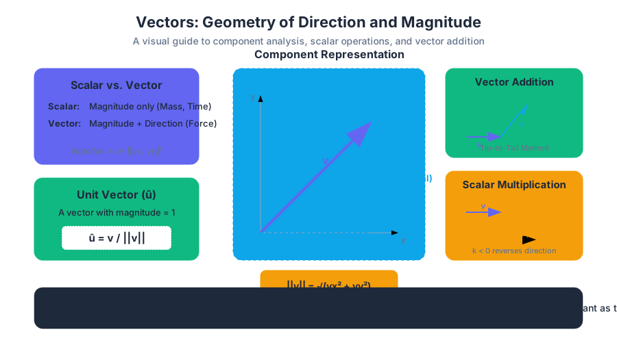
In the study of mathematics and physics, we distinguish between two fundamental types of quantities: scalars and vectors. While a scalar is defined solely by its magnitude (such as temperature, mass, or time), a vector is a mathematical object that possesses both magnitude and direction.
In a Euclidean space, a vector is often visualized as a directed line segment—an arrow—starting at an initial point and ending at a terminal point. However, in modern linear algebra and engineering, we treat vectors more abstractly as elements of a vector space, typically represented by their components in a coordinate system. This section explores the rigorous foundations of vector algebra, from basic component analysis to the nuances of polar-rectangular conversions.
Vector Components and Magnitude
At its core, a vector in $\mathbb{R}^2$ or $\mathbb{R}^3$ can be decomposed into its constituent parts along the axes of a coordinate system. These parts are known as components.
The Component Representation
If a vector $\vec{v}$ has its initial point at the origin $(0,0)$ and its terminal point at $(x, y)$, we say the vector is in standard position. The component form is written as: $$\vec{v} = \langle v_x, v_y \rangle$$ where $v_x$ is the horizontal displacement and $v_y$ is the vertical displacement. In three dimensions, this extends to $\vec{v} = \langle v_x, v_y, v_z \rangle$.
Calculating Magnitude
The magnitude (or norm) of a vector, denoted as $|\vec{v}|$, represents the length of the directed line segment. By the Pythagorean theorem, the magnitude of a 2D vector is the square root of the sum of the squares of its components: $$|\vec{v}| = \sqrt{v_x^2 + v_y^2}$$
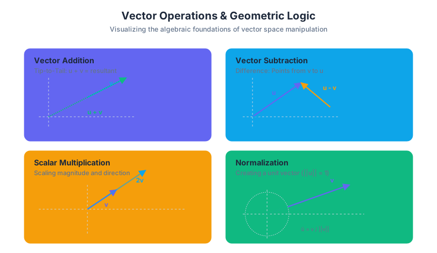
Definition: The Unit Vector A unit vector is a vector with a magnitude of exactly 1. Any non-zero vector $\vec{v}$ can be "normalized" into a unit vector $\hat{u}$ by dividing the vector by its magnitude: $$\hat{u} = \frac{\vec{v}}{|\vec{v}|}$$
| Property | Scalar | Vector |
|---|---|---|
| Definition | Magnitude only | Magnitude and Direction |
| Examples | Speed, Mass, Energy | Velocity, Force, Acceleration |
| Notation | $s$ (italic) | $\vec{v}$ or v (bold/arrow) |
| Dimensionality | 1D (Rank 0 Tensor) | n-D (Rank 1 Tensor) |
Scalar Multiplication
Scalar multiplication involves changing the magnitude (and potentially the direction) of a vector by multiplying it by a real number $k$.
Mechanics of Scaling
When a vector $\vec{v} = \langle x, y \rangle$ is multiplied by a scalar $k$, the operation is applied component-wise: $$k\vec{v} = \langle kx, ky \rangle$$
The effect on the vector depends on the value of $k$:
- If $k > 1$: The vector is stretched (dilated).
- If $0 < k < 1$: The vector is shrunk (compressed).
- If $k = 0$: The vector becomes the zero vector $\vec{0} = \langle 0, 0 \rangle$.
- If $k < 0$: The vector's direction is reversed ($180^\circ$ flip) and its magnitude is scaled by $|k|$.
Geometric Interpretation
Geometrically, scalar multiplication keeps the vector on the same line of action (it remains parallel to the original) but alters its reach. This is fundamental in defining collinearity: two vectors are parallel if and only if one is a scalar multiple of the other.
Vector Addition and Subtraction
Vector addition is not as simple as adding magnitudes. Because vectors have direction, we must account for their spatial orientation using either geometric or algebraic methods.
The Tip-to-Tail Method (Geometric)
To add $\vec{u}$ and $\vec{v}$ geometrically:
- Draw vector $\vec{u}$.
- Place the initial point (tail) of $\vec{v}$ at the terminal point (tip) of $\vec{u}$.
- The resultant vector $\vec{u} + \vec{v}$ is the vector drawn from the tail of $\vec{u}$ to the tip of $\vec{v}$.
Component-wise Addition (Algebraic)
Algebraically, addition is performed by summing the corresponding components: $$\vec{u} + \vec{v} = \langle u_x + v_x, u_y + v_y \rangle$$
Vector Subtraction
Subtraction is defined as the addition of a negative vector: $\vec{u} - \vec{v} = \vec{u} + (-\vec{v})$. Geometrically, if $\vec{u}$ and $\vec{v}$ share the same initial point, $\vec{u} - \vec{v}$ is the vector pointing from the tip of $\vec{v}$ to the tip of $\vec{u}$.
| Operation | Algebraic Formula | Geometric Meaning |
|---|---|---|
| Addition | $\langle x_1+x_2, y_1+y_2 \rangle$ | Diagonal of a parallelogram |
| Subtraction | $\langle x_1-x_2, y_1-y_2 \rangle$ | Vector connecting two points |
| Scalar Mult. | $\langle kx, ky \rangle$ | Resizing the vector |
| Normalization | $\langle \frac{x}{|\vec{v}|}, \frac{y}{|\vec{v}|} \rangle$ | Finding the direction unit |
Implementation: Vector Arithmetic in Python
In scientific computing, we rarely implement these manually. We use optimized libraries like NumPy, which treat vectors as arrays.
import numpy as np

def vector_analysis(u_coords, v_coords, scalar):
    """
    Performs fundamental vector operations using NumPy.
    """
    u = np.array(u_coords)
    v = np.array(v_coords)

    # Addition and Subtraction
    v_sum = u + v
    v_diff = u - v

    # Scalar Multiplication
    v_scaled = scalar * u

    # Magnitude (L2 Norm)
    mag_u = np.linalg.norm(u)

    # Normalization (Unit Vector)
    unit_u = u / mag_u if mag_u != 0 else u

    return {
        "sum": v_sum,
        "diff": v_diff,
        "scaled": v_scaled,
        "magnitude": mag_u,
        "unit": unit_u
    }

# Example usage:
# u = <3, 4>, v = <1, 2>, k = 2
results = vector_analysis([3, 4], [1, 2], 2)
print(f"Resultant: {results['sum']}") # Expected: [4, 6]
Rectangular and Polar Conversion
While rectangular coordinates (Cartesian) are excellent for addition and subtraction, polar coordinates are often more intuitive for describing movement, such as a plane flying at a certain heading or a force applied at an angle.
From Polar to Rectangular
A vector in polar form is defined by its magnitude $r$ and its direction angle $\theta$ (usually measured counter-clockwise from the positive x-axis). To find the components: $$x = r \cos \theta$$ $$y = r \sin \theta$$
From Rectangular to Polar
To convert from components $\langle x, y \rangle$ back to $(r, \theta)$:
- Magnitude: $r = \sqrt{x^2 + y^2}$
- Direction: $\theta = \tan^{-1}\left(\frac{y}{x}\right)$
The Quadrant Warning The standard
arctanfunction only returns values in the range $(-\pi/2, \pi/2)$. If your vector is in the second or third quadrant ($x < 0$), you must add $180^\circ$ (or $\pi$ radians) to the result to get the correct direction. In programming, theatan2(y, x)function handles this logic automatically.
Mathematical Derivation: The Rotation Matrix
If we wish to rotate a vector $\vec{v}$ by an angle $\phi$, we can derive the new coordinates using the polar conversion logic.
Let v = <r cos(theta), r sin(theta)>
After rotating by phi, the new angle is (theta + phi).
x' = r cos(theta + phi) = r(cos theta cos phi - sin theta sin phi)
y' = r sin(theta + phi) = r(sin theta cos phi + cos theta sin phi)

Substituting x = r cos theta and y = r sin theta:
x' = x cos phi - y sin phi
y' = x sin phi + y cos phi

This yields the Rotation Matrix R:
[ x' ]   [ cos phi  -sin phi ] [ x ]
[ y' ] = [ sin phi   cos phi ] [ y ]
Practical Applications and Worked Examples
Case Study: Resultant Velocity
An airplane is flying at an airspeed of 500 km/h at a bearing of $30^\circ$ North of East. A wind is blowing from the South at 80 km/h. What is the ground speed and actual direction of the plane?
Step 1: Convert to Rectangular Components
- Plane ($\vec{p}$): $r=500, \theta=30^\circ$
- $p_x = 500 \cos(30^\circ) \approx 433.01$
- $p_y = 500 \sin(30^\circ) = 250$
- Wind ($\vec{w}$): $r=80, \theta=90^\circ$ (From South means blowing North)
- $w_x = 80 \cos(90^\circ) = 0$
- $w_y = 80 \sin(90^\circ) = 80$
Step 2: Add Components
- $\vec{R} = \vec{p} + \vec{w} = \langle 433.01 + 0, 250 + 80 \rangle = \langle 433.01, 330 \rangle$
Step 3: Convert back to Polar
- Ground Speed: $|\vec{R}| = \sqrt{433.01^2 + 330^2} \approx 544.4$ km/h
- Direction: $\theta = \tan^{-1}(330 / 433.01) \approx 37.3^\circ$ North of East.
Real-World Usage: Physics Engine Update (C++)
In game development, vectors are used to update the position of objects based on velocity and acceleration.
#include <iostream>
#include <cmath>

struct Vector2D {
    float x, y;

    // Vector Addition
    Vector2D operator+(const Vector2D& other) const {
        return {x + other.x, y + other.y};
    }

    // Scalar Multiplication
    Vector2D operator*(float scalar) const {
        return {x * scalar, y * scalar};
    }
};

int main() {
    Vector2D position = {0.0f, 0.0f};
    Vector2D velocity = {10.0f, 5.0f}; // Units per second
    float deltaTime = 0.016f; // Simulation step (60 FPS)

    // Euler Integration: pos = pos + vel * dt
    for(int frame = 0; frame < 60; ++frame) {
        position = position + (velocity * deltaTime);
    }

    std::cout << "Final Position: (" << position.x << ", " << position.y << ")" << std::endl;
    return 0;
}
Common Pitfalls and Edge Cases
- Confusing Bearing with Standard Angle: In navigation, "Bearing" is often measured clockwise from North. In mathematics, $\theta$ is measured counter-clockwise from the positive X-axis (East). Always convert bearings to standard angles before using $\sin$ and $\cos$.
- Magnitude of Subtraction: Beginners often think $|\vec{u} - \vec{v}| = |\vec{u}| - |\vec{v}|$. This is false. The magnitude of the difference depends on the angle between the vectors (Law of Cosines).
- Floating Point Precision: When comparing if two vectors are equal or if a vector is a unit vector, always use an epsilon ($\epsilon$) threshold rather than
== 1.0due to rounding errors insqrtandtrigfunctions.
| Feature | Rectangular (Cartesian) | Polar |
|---|---|---|
| Best For | Addition, Subtraction, Integration | Rotation, Circular Motion, Navigation |
| Components | $x, y$ | $r, \theta$ |
| Zero Vector | $\langle 0, 0 \rangle$ | $r=0, \theta$ is undefined |
| Uniqueness | Unique representation | Multiple (e.g., $\theta$ vs $\theta + 2\pi$) |
Summary of Key Formulas
| Concept | Formula |
|---|---|
| Magnitude | $|\vec{v}| = \sqrt{x^2 + y^2}$ |
| Unit Vector | $\hat{u} = \frac{1}{|\vec{v}|} \langle x, y \rangle$ |
| Addition | $\vec{u} + \vec{v} = \langle u_x + v_x, u_y + v_y \rangle$ |
| Scalar Mult. | $k\vec{v} = \langle kx, ky \rangle$ |
| X-Component | $x = r \cos \theta$ |
| Y-Component | $y = r \sin \theta$ |
| Angle | $\theta = \operatorname{atan2}(y, x)$ |
Matrices
Key concepts: Matrix multiplication · Geometric transformations · Determinants and area · Inverse matrices
Covers matrix algebra, determinants, and the use of inverse matrices to solve systems of linear equations and perform geometric transformations.
Matrices: The Engines of Linear Algebra
In the landscape of modern mathematics, a matrix is far more than a simple grid of numbers. While a novice might view a matrix as a static data structure—a spreadsheet of values—a mathematician or engineer views it as a linear operator. It is a machine that takes a vector and transforms it into another vector, preserving the origin and the parallelism of lines.
From the perspective of computational science, matrices are the fundamental language of the physical world. Whether you are simulating the stress on a bridge, rendering a 3D character in a video game, or training a neural network with billions of parameters, you are performing matrix operations. This article explores the mechanics of these operations, the geometric intuition behind them, and the algebraic structures that allow us to "undo" transformations.
1. Matrix Multiplication: The Composition of Operators
Matrix multiplication is the most fundamental operation in linear algebra, yet it is often the most misunderstood by beginners. Unlike addition, which is performed element-wise, multiplication is a compositional process.
1.1 The Mechanics: Row-by-Column
To multiply two matrices $A$ and $B$, the number of columns in $A$ must equal the number of rows in $B$. If $A$ is an $m \times n$ matrix and $B$ is $n \times p$, the resulting matrix $C$ will be $m \times p$. Each element $c_{ij}$ is the dot product of the $i$-th row of $A$ and the $j$-th column of $B$.
Definition: Matrix Multiplication For matrices $A$ (size $m \times n$) and $B$ (size $n \times p$), the product $C = AB$ is defined by: $$c_{ij} = \sum_{k=1}^{n} a_{ik}b_{kj}$$
1.2 Properties and Constraints
The most critical realization in matrix algebra is that multiplication is non-commutative. In almost all cases, $AB \neq BA$. Geometrically, this makes sense: if you rotate a cube and then slide it, you end up in a different position than if you slid it first and then rotated it.
| Property | Formula | Description |
|---|---|---|
| Non-Commutative | $AB \neq BA$ | The order of operations matters significantly. |
| Associative | $A(BC) = (AB)C$ | Grouping does not change the result. |
| Distributive | $A(B + C) = AB + AC$ | Multiplication distributes over addition. |
| Identity | $AI = IA = A$ | Multiplying by the Identity matrix leaves the matrix unchanged. |
1.3 Implementation in High-Level Scientific Computing
In modern data science, we rarely implement the summation manually. Libraries like NumPy use highly optimized BLAS (Basic Linear Algebra Subprograms) to handle these operations.
import numpy as np

# Define two matrices
# A is 2x3, B is 3x2
A = np.array([[1, 2, 3],
              [4, 5, 6]])

B = np.array([[7, 8],
              [9, 10],
              [11, 12]])

# Standard matrix multiplication using the @ operator (Python 3.5+)
# Result will be a 2x2 matrix
C = A @ B

print(f"Matrix A shape: {A.shape}")
print(f"Matrix B shape: {B.shape}")
print(f"Resulting Matrix C:\n{C}")

# Verification of non-commutativity
try:
    D = B @ A
    print(f"\nB @ A is possible and results in a {D.shape} matrix.")
    print("Notice that C (2x2) and D (3x3) are entirely different shapes!")
except ValueError as e:
    print(f"B @ A failed: {e}")
2. Geometric Transformations: Mapping the Plane
If we treat a $2 \times 2$ matrix as a function, its input is a vector $(x, y)$ and its output is a new vector $(x', y')$. This is the foundation of computer graphics. Every matrix represents a linear transformation.
2.1 The Basis Vector Intuition
To understand what a matrix does, you only need to look at what it does to the basis vectors: $\hat{i}$ (the unit vector on the x-axis, $[1, 0]$) and $\hat{j}$ (the unit vector on the y-axis, $[0, 1]$).
If a matrix $M$ is: $$ M =
\begin{bmatrix} a & b \ c & d \end{bmatrix} $$ The first column $[a, c]^T$ tells you where $\hat{i}$ lands, and the second column $[b, d]^T$ tells you where $\hat{j}$ lands. Every other point in the plane follows them linearly.
2.2 Common 2D Transformations
By manipulating these basis vectors, we can derive standard transformation matrices.
| Transformation | Matrix Representation | Effect |
|---|---|---|
| Scaling | $\begin{bmatrix} s_x & 0 \ 0 & s_y \end{bmatrix}$ | Stretches or shrinks the plane along axes. |
| Rotation ($\theta$) | $\begin{bmatrix} \cos\theta & -\sin\theta \ \sin\theta & \cos\theta \end{bmatrix}$ | Rotates the plane counter-clockwise by $\theta$. |
| Shear (Horizontal) | $\begin{bmatrix} 1 & k \ 0 & 1 \end{bmatrix}$ | Slides the top of the plane to the right by factor $k$. |
| Reflection (X-axis) | $\begin{bmatrix} 1 & 0 \ 0 & -1 \end{bmatrix}$ | Flips the plane over the x-axis. |
2.3 Mathematical Derivation of Rotation
To derive the rotation matrix, we consider where $\hat{i} = (1, 0)$ and $\hat{j} = (0, 1)$ move when rotated by $\theta$ on the unit circle.
\text{Step 1: Rotate } \hat{i} (1, 0)
\text{New position: } (\cos\theta, \sin\theta)

\text{Step 2: Rotate } \hat{j} (0, 1)
\text{New position: } (-\sin\theta, \cos\theta)

\text{Step 3: Construct Matrix } R
R = \begin{bmatrix} \text{new } \hat{i} & \text{new } \hat{j} \end{bmatrix} = \begin{bmatrix} \cos\theta & -\sin\theta \\ \sin\theta & \cos\theta \end{bmatrix}
3. Determinants: The Scaling Factor of Space
The determinant of a matrix, denoted as $\det(A)$ or $|A|$, is a scalar value that encodes how much the transformation changes areas (in 2D) or volumes (in 3D).
3.1 Geometric Interpretation
If you take a unit square (area = 1) and apply a transformation $A$, the area of the resulting parallelogram is exactly $|\det(A)|$.
- If $\det(A) = 2$, the transformation doubles the area of any shape.
- If $\det(A) = 0.5$, the area is halved.
- If $\det(A) = 0$, the transformation collapses the space into a lower dimension (a line or a point). This means the matrix is singular and has no inverse.
- If $\det(A) < 0$, the orientation of the space has been flipped (like looking in a mirror).
3.2 Calculation Methods
For a $2 \times 2$ matrix, the calculation is straightforward: $$ \det \begin{bmatrix} a & b \ c & d \end{bmatrix}
= ad - bc $$
For a $3 \times 3$ matrix, we use Laplace Expansion (expansion by minors): $$ \det
\begin{bmatrix} a & b & c \ d & e & f \ g & h & i \end{bmatrix}
= a(ei - fh) - b(di - fg) + c(dh - eg) $$
| Determinant Value | Geometric Meaning | Algebraic Meaning |
|---|---|---|
| $\det(A) \neq 0$ | Space is preserved; no collapse. | Matrix is Invertible. |
| $\det(A) = 0$ | Space collapses (Line/Point). | Matrix is Singular (Non-invertible). |
| $\det(A) = 1$ | Area/Volume is preserved. | Transformation is Equiareal. |
| $\det(A) = -1$ | Area preserved, orientation flipped. | Reflection-like transformation. |
4. Inverse Matrices: Reversing the Transformation
If a matrix $A$ represents a transformation, the inverse matrix $A^{-1}$ represents the transformation that "undoes" $A$. If you apply $A$ and then $A^{-1}$, you return to your starting position.
4.1 The Identity Matrix
The identity matrix $I$ is the "1" of the matrix world. It has 1s on the main diagonal and 0s elsewhere. $$A A^{-1} = A^{-1} A = I$$
4.2 Finding the Inverse ($2 \times 2$ Case)
For a $2 \times 2$ matrix $A = \begin{bmatrix} a & b \ c & d \end{bmatrix}$, the inverse is: $$A^{-1} = \frac{1}{\det(A)} \begin{bmatrix} d & -b \ -c & a \end{bmatrix}$$ Observe that if $\det(A) = 0$, we would be dividing by zero, which confirms why singular matrices cannot be inverted.
4.3 Low-Level Implementation in C
In systems programming or embedded graphics, we often implement these formulas directly to avoid the overhead of heavy libraries.
#include <stdio.h>
#include <stdbool.h>

typedef struct {
    double data[2][2];
} Matrix2x2;

/**
 * Calculates the inverse of a 2x2 matrix.
 * Returns true if successful, false if matrix is singular.
 */
bool invert_matrix(Matrix2x2 src, Matrix2x2 *dest) {
    double det = (src.data[0][0] * src.data[1][1]) -
                 (src.data[0][1] * src.data[1][0]);

    // Check for singularity with a small epsilon for floating point safety
    if (det > -1e-9 && det < 1e-9) {
        return false;
    }

    double inv_det = 1.0 / det;

    dest->data[0][0] =  src.data[1][1] * inv_det;
    dest->data[0][1] = -src.data[0][1] * inv_det;
    dest->data[1][0] = -src.data[1][0] * inv_det;
    dest->data[1][1] =  src.data[0][0] * inv_det;

    return true;
}

int main() {
    Matrix2x2 A = {{{4, 7}, {2, 6}}};
    Matrix2x2 A_inv;

    if (invert_matrix(A, &A_inv)) {
        printf("Inverse Matrix:\n");
        printf("[%f, %f]\n[%f, %f]\n",
               A_inv.data[0][0], A_inv.data[0][1],
               A_inv.data[1][0], A_inv.data[1][1]);
    } else {
        printf("Matrix is singular and cannot be inverted.\n");
    }
    return 0;
}
5. Solving Systems of Linear Equations
One of the primary motivations for studying matrices is the ability to solve systems of equations of the form: $$a_{11}x_1 + a_{12}x_2 = b_1$$ $$a_{21}x_1 + a_{22}x_2 = b_2$$
This can be written as a single matrix equation: $AX = B$.
5.1 The Matrix Solution
If $A$ is invertible, we can solve for the vector of unknowns $X$ by multiplying both sides by $A^{-1}$: $$A^{-1}(AX) = A^{-1}B$$ $$IX = A^{-1}B$$ $$X = A^{-1}B$$
5.2 Comparison of Solving Methods
While $X = A^{-1}B$ is conceptually elegant, it is not always the most efficient way to solve a system numerically.
| Method | Best For | Complexity | Pros/Cons |
|---|---|---|---|
| Matrix Inversion | Theoretical derivation | $O(n^3)$ | Easy to write; numerically unstable for large $n$. |
| Gaussian Elimination | Small to medium systems | $O(n^3)$ | Robust; standard for manual calculation. |
| LU Decomposition | Multiple $B$ vectors | $O(n^3)$ | Efficient if $A$ stays the same but $B$ changes. |
| Iterative (Jacobi/GS) | Massive sparse matrices | $O(kn^2)$ | Used in physics simulations and "Big Data". |
5.3 Real-World Usage: Solving via CLI
Engineers often use command-line tools or specialized languages like Julia or MATLAB for quick system solving.
# Using 'octave' (the open-source MATLAB alternative) to solve AX = B
# A = [3 2; 1 2], B = [10; 6]

octave --eval "A=[3,2; 1,2]; B=[10;6]; X=A\B; disp(X)"

# Output:
#   2
#   2
# This solves:
# 3x + 2y = 10
# 1x + 2y = 6
# Result: x=2, y=2
6. Common Pitfalls and Advanced Concepts
6.1 The "Division" Fallacy
Students often ask, "How do I divide by a matrix?" There is no such thing as matrix division. You must use the inverse. Furthermore, because multiplication is non-commutative, you must specify if you are "pre-multiplying" or "post-multiplying."
- $AX = B \implies X = A^{-1}B$ (Correct)
- $AX = B \implies X = BA^{-1}$ (Incorrect)
6.2 Floating Point Errors
In computational practice, a determinant might not be exactly zero due to rounding errors, but it might be "effectively zero." This is known as a poorly conditioned matrix. The Condition Number of a matrix measures how sensitive the output is to small changes in the input.
6.3 Eigenvalues and Eigenvectors
Beyond basic transformations, we look for vectors that do not change direction when a transformation is applied—only their scale changes. These are eigenvectors, and their scaling factor is the eigenvalue. This is the secret sauce behind Google's PageRank algorithm and Principal Component Analysis (PCA).
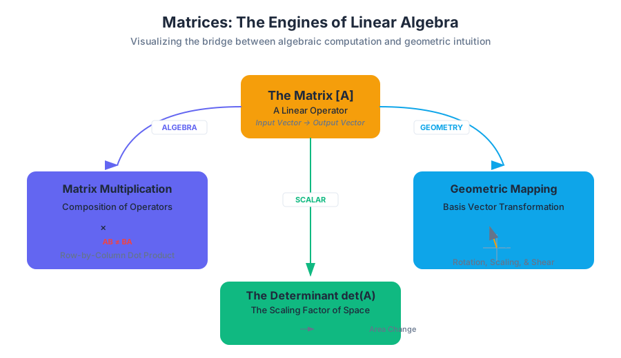
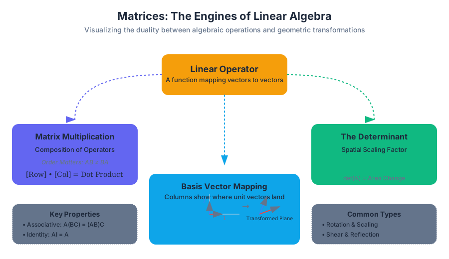
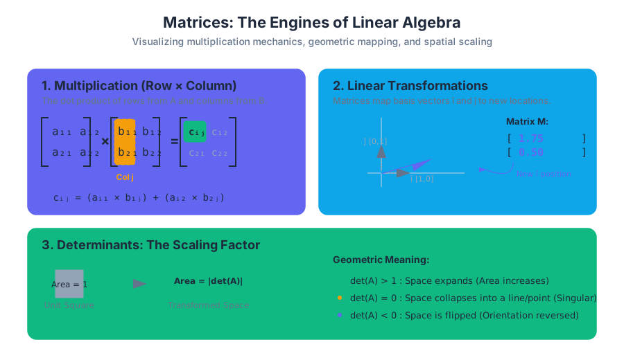
Probability and Combinatorics
Key concepts: Permutations and combinations · Addition and multiplication rules · Discrete probability distributions · Expected value
Explores counting methods and the rules of probability for compound events and discrete random variables.
Probability and Combinatorics
The study of probability and combinatorics represents the mathematical science of uncertainty and arrangement. While combinatorics provides the tools to count the number of ways discrete events can occur, probability provides the measure of how likely those events are to happen within a defined sample space. To the engineer, these are the tools of risk assessment and reliability; to the data scientist, they are the bedrock of inference; and to the mathematician, they are a beautiful exploration of the structure of sets.
The Calculus of Counting: Combinatorics
Combinatorics is often called "the art of counting without counting." When dealing with large sets, manual enumeration is impossible. Instead, we rely on fundamental principles to derive the size of a sample space or the number of successful outcomes.
The Fundamental Counting Principle
The Fundamental Counting Principle (or the Multiplication Rule for counting) states that if one task can be performed in $n$ ways and a second task can be performed in $m$ ways, then the sequence of two tasks can be performed in $n \times m$ ways. This generalizes to any number of tasks.
Permutations: When Order Defines Identity
A Permutation is an ordered arrangement of a subset of items. In a permutation, the sequence matters: the arrangement $(A, B)$ is distinct from $(B, A)$.
Definition: The Permutation Formula The number of ways to arrange $r$ objects from a set of $n$ distinct objects is given by: $$P(n, r) = \frac{n!}{(n-r)!}$$ where $n!$ (n-factorial) represents the product of all positive integers up to $n$.
Why the division? We start with $n$ choices for the first position, $n-1$ for the second, and so on, until we have filled $r$ positions. The $(n-r)!$ in the denominator "cancels out" the choices we didn't make, leaving only the $r$ factors.
Combinations: The Logic of Selection
A Combination is a selection of items where the order does not matter. If you are choosing a committee of three people from a group of ten, the order in which you pick them is irrelevant; the resulting group is the same.
Definition: The Combination Formula The number of ways to choose $r$ objects from $n$ distinct objects is: $$C(n, r) = \binom{n}{r} = \frac{n!}{r!(n-r)!}$$
The Intuition: A combination is simply a permutation where we have "divided out" the redundant orderings. Since there are $r!$ ways to arrange $r$ objects, dividing $P(n, r)$ by $r!$ removes the significance of the sequence.
| Feature | Permutation ($P$) | Combination ($C$) |
|---|---|---|
| Order Matters? | Yes | No |
| Key Keyword | Arrange, Sequence, Order | Select, Choose, Group |
| Formula | $\frac{n!}{(n-r)!}$ | $\frac{n!}{r!(n-r)!}$ |
| Result Size | Larger | Smaller |
| Example | Race finish (1st, 2nd, 3rd) | Hand of cards |
Advanced Combinatorics: Repetition and Constraints
In real-world scenarios, we often encounter "Permutations with Repetition" (e.g., arranging the letters in "MISSISSIPPI") or "Combinations with Repetition" (e.g., picking 5 pieces of fruit from a basket of apples, oranges, and bananas).
- Permutations with Indistinguishable Objects: If there are $n$ total objects where $n_1$ are of one type, $n_2$ of another, etc., the total permutations are $\frac{n!}{n_1! n_2! \dots n_k!}$.
- Stars and Bars (Combinations with Repetition): The number of ways to choose $r$ items from $n$ types with replacement is $\binom{n+r-1}{r}$.
import math

def calculate_combinatorics(n, r):
    """
    A low-level implementation of permutation and combination logic.
    Uses math.factorial for precision with large integers.
    """
    if r > n or r < 0:
        return 0, 0

    # nPr = n! / (n-r)!
    permutation = math.factorial(n) // math.factorial(n - r)

    # nCr = n! / (r! * (n-r)!)
    combination = permutation // math.factorial(r)

    return permutation, combination

# Example: Choosing 3 cards from a deck of 52
n, r = 52, 3
p, c = calculate_combinatorics(n, r)

print(f"Permutations (Order matters): {p:,}") # 132,600
print(f"Combinations (Order doesn't matter): {c:,}") # 22,100
The Rules of Probability
Probability is the ratio of the size of the event space to the size of the sample space, assuming all outcomes are equally likely: $P(E) = \frac{|E|}{|S|}$.
The Addition Rule (OR Logic)
The Addition Rule is used when we want to find the probability that either Event A or Event B occurs.
- Mutually Exclusive Events: If A and B cannot happen at the same time ($A \cap B = \emptyset$), then: $$P(A \cup B) = P(A) + P(B)$$
- General Addition Rule (Inclusion-Exclusion): If the events can overlap, we must subtract the intersection to avoid double-counting: $$P(A \cup B) = P(A) + P(B) - P(A \cap B)$$
The Multiplication Rule (AND Logic)
The Multiplication Rule is used to find the probability that both Event A and Event B occur.
- Independent Events: If the occurrence of A does not change the probability of B: $$P(A \cap B) = P(A) \times P(B)$$
- Dependent Events (Conditional Probability): If the occurrence of A affects B: $$P(A \cap B) = P(A) \times P(B|A)$$ Where $P(B|A)$ is the probability of B given that A has already occurred.
\begin{aligned}
&\text{Derivation of Bayes' Theorem from the Multiplication Rule:} \\
\\
&1. \quad P(A \cap B) = P(A|B)P(B) \\
&2. \quad P(B \cap A) = P(B|A)P(A) \\
&\text{Since } P(A \cap B) = P(B \cap A): \\
&3. \quad P(A|B)P(B) = P(B|A)P(A) \\
&4. \quad P(A|B) = \frac{P(B|A)P(A)}{P(B)}
\end{aligned}
Discrete Probability Distributions
A Random Variable is a numerical description of the outcome of a statistical experiment. When the possible values are countable (e.g., 0, 1, 2, ...), we call it a Discrete Random Variable.
Probability Mass Function (PMF)
The Probability Mass Function (PMF), denoted as $f(x) = P(X = x)$, maps every possible value of a discrete random variable to its probability.
Axioms of Probability Distributions:
- $0 \le P(X=x) \le 1$ for all $x$.
- $\sum P(X=x) = 1$ (The sum of all probabilities in the sample space must be unity).
Common Discrete Distributions
| Distribution | Use Case | Parameters | PMF Formula |
|---|---|---|---|
| Bernoulli | Single trial with two outcomes (Success/Failure) | $p$ (prob of success) | $p^x(1-p)^{1-x}$ |
| Binomial | Number of successes in $n$ independent trials | $n, p$ | $\binom{n}{k} p^k (1-p)^{n-k}$ |
| Poisson | Number of events in a fixed interval of time/space | $\lambda$ (average rate) | $\frac{e^{-\lambda} \lambda^k}{k!}$ |
| Geometric | Number of trials until the first success | $p$ | $(1-p)^{k-1}p$ |
Worked Example: The Binomial Distribution
Imagine a software system where each request has a 1% chance of failing ($p=0.01$). If the system receives 100 requests, what is the probability that exactly 2 fail?
Using the Binomial PMF: $P(X=2) = \binom{100}{2} (0.01)^2 (0.99)^{98}$ $P(X=2) = 4950 \times 0.0001 \times 0.373 = 0.1848$ (approx 18.5%).
Expected Value and Variance
The Expected Value $E[X]$ is the long-term arithmetic mean of a random variable. It represents the "center of mass" of the distribution.
Calculating Expected Value
For a discrete random variable $X$: $$E[X] = \mu = \sum_{i=1}^{n} x_i P(x_i)$$
It is the weighted average where the weights are the probabilities of each outcome.
Linearity of Expectation
One of the most powerful properties in probability is Linearity of Expectation, which states that the expected value of the sum of random variables is the sum of their expected values, regardless of whether they are independent: $$E[X + Y] = E[X] + E[Y]$$
Variance and Standard Deviation
While the expected value tells us where the distribution is centered, Variance ($\sigma^2$) tells us how "spread out" the values are. $$Var(X) = E[(X - \mu)^2] = E[X^2] - (E[X])^2$$ The Standard Deviation ($\sigma$) is simply the square root of the variance, bringing the units back to the same scale as the original variable.
-- Real-world usage: Calculating Expected Value from a Database
-- Scenario: A gaming company wants to calculate the 'Expected Revenue'
-- per user based on purchase history and probability of conversion.

SELECT
    user_segment,
    SUM(item_price * purchase_probability) AS expected_revenue_per_user,
    SQRT(SUM(POWER(item_price, 2) * purchase_probability) - POWER(SUM(item_price * purchase_probability), 2)) AS std_dev_revenue
FROM
    marketing_predictions
GROUP BY
    user_segment;
Common Pitfalls and Paradoxes
Probability is notoriously counter-intuitive. Even experts frequently fall into mental traps.
- The Gambler's Fallacy: The mistaken belief that if an event happens more frequently than normal during a given period, it will happen less frequently in the future (and vice-versa). If a fair coin lands heads 10 times in a row, the probability of tails on the 11th flip is still exactly 0.5.
- The Birthday Paradox: In a room of just 23 people, there is a >50% chance that two of them share a birthday. This happens because we are looking for any pair of people to match, and the number of pairs grows quadratically ($C(23, 2) = 253$).
- Confusing Mutually Exclusive with Independent:
- Mutually Exclusive: If A happens, B cannot happen. They are highly dependent.
- Independent: If A happens, it tells you nothing about whether B will happen.
Summary of Key Formulas
| Concept | Formula |
|---|---|
| Permutations | $P(n, r) = \frac{n!}{(n-r)!}$ |
| Combinations | $C(n, r) = \frac{n!}{r!(n-r)!}$ |
| General Addition | $P(A \cup B) = P(A) + P(B) - P(A \cap B)$ |
| Conditional Prob | $P(A\vert B) = \frac{P(A \cap B)}{P(B)}$ |
| Expected Value | $E[X] = \sum x P(x)$ |
| Variance | $Var(X) = \sum (x - \mu)^2 P(x)$ |
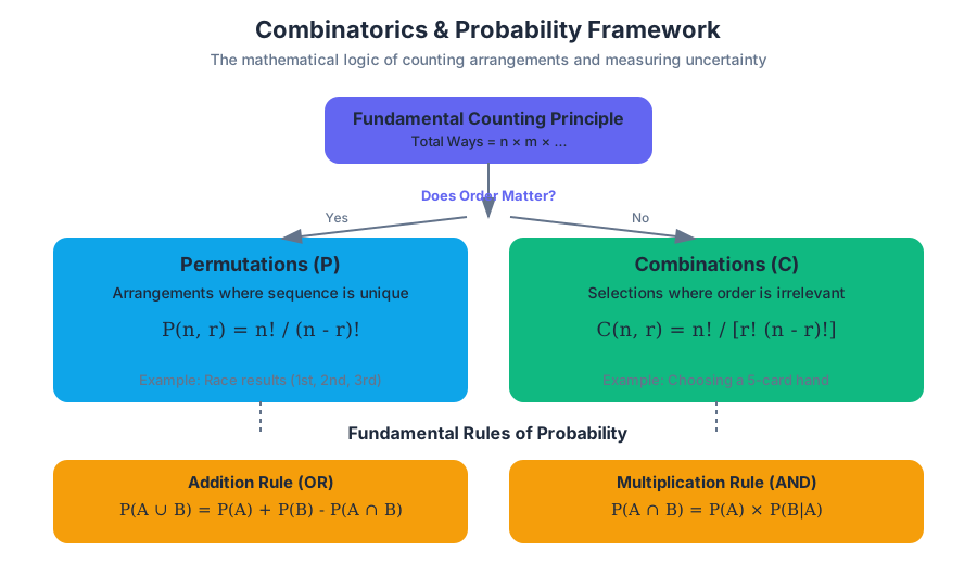
Series and Binomial Theorem
Key concepts: Arithmetic and geometric series · Sigma (Σ) notation · Binomial theorem · Pascal's triangle
Focuses on arithmetic and geometric series, summation notation, and the expansion of binomial expressions using Pascal's Triangle.
Series and Binomial Theorem
The study of series and the Binomial Theorem represents a critical transition point in mathematics. It is here that we move from the static world of individual numbers and simple algebraic expressions into the dynamic realm of infinite processes and combinatorial structures. In essence, a series is the sum of the terms of a sequence, while the Binomial Theorem provides a powerful algebraic shortcut for expanding powers of binomials.
These concepts are not merely academic exercises; they form the bedrock of modern finance (calculating compound interest and annuities), physics (approximating complex wave functions), and computer science (analyzing algorithm complexity and data structures).
The Language of Summation: Sigma (Σ) Notation
Before diving into specific types of series, we must master the notation used to describe them. Sigma notation is a concise way to represent the sum of many terms that follow a specific pattern.
Definition: Sigma Notation The expression $\sum_{i=k}^{n} a_i$ denotes the sum of terms $a_i$ starting from the index $i=k$ and ending at $i=n$.
- $\Sigma$ (Sigma): The Greek capital letter for "S," standing for "Sum."
- $i$: The index of summation (the "counter").
- $k$: The lower limit (starting value).
- $n$: The upper limit (ending value).
- $a_i$: The general term or formula for the $i$-th element.
Properties of Summation
To manipulate series effectively, we rely on several fundamental properties:
| Property | Mathematical Expression | Description |
|---|---|---|
| Linearity (Scalar) | $\sum ca_i = c \sum a_i$ | Constants can be factored out of the summation. |
| Linearity (Addition) | $\sum (a_i + b_i) = \sum a_i + \sum b_i$ | The sum of a sum is the sum of the individual sums. |
| Constant Sum | $\sum_{i=1}^{n} c = nc$ | Adding a constant $c$ to itself $n$ times is $n \times c$. |
| Index Shifting | $\sum_{i=1}^{n} a_i = \sum_{i=0}^{n-1} a_{i+1}$ | The index can be adjusted as long as the terms remain identical. |
Arithmetic Series: Linear Accumulation
An Arithmetic Series is the sum of the terms of an arithmetic sequence—a sequence where the difference between consecutive terms is constant. This constant is known as the common difference ($d$).
The Sum Formula
The sum of the first $n$ terms of an arithmetic series ($S_n$) is given by: $$S_n = \frac{n}{2}(a_1 + a_n)$$ Alternatively, by substituting the formula for the $n$-th term ($a_n = a_1 + (n-1)d$), we get: $$S_n = \frac{n}{2}[2a_1 + (n-1)d]$$
Derivation: The Gaussian Trick
Legend has it that Carl Friedrich Gauss, as a young student, was asked to sum the numbers from 1 to 100. He realized that if you write the series twice—once forward and once backward—and add the columns, each column sums to the same value.
- $S_n = a_1 + (a_1 + d) + (a_1 + 2d) + \dots + a_n$
- $S_n = a_n + (a_n - d) + (a_n - 2d) + \dots + a_1$
- $2S_n = (a_1 + a_n) + (a_1 + a_n) + \dots + (a_1 + a_n)$
- $2S_n = n(a_1 + a_n) \implies S_n = \frac{n}{2}(a_1 + a_n)$
def arithmetic_series_sum(a1, d, n):
    """
    Calculates the sum of an arithmetic series.

    Parameters:
    a1 (float): The first term
    d (float): The common difference
    n (int): Number of terms

    Returns:
    float: The sum of the first n terms
    """
    # Using the derived formula for O(1) complexity
    if n <= 0:
        return 0

    an = a1 + (n - 1) * d
    sn = (n / 2) * (a1 + an)
    return sn

# Example: Sum of 1 to 100
# a1 = 1, d = 1, n = 100
print(f"Sum of 1 to 100: {arithmetic_series_sum(1, 1, 100)}")
Geometric Series: Exponential Accumulation
A Geometric Series is the sum of the terms of a geometric sequence, where each term is found by multiplying the previous term by a common ratio ($r$).
Finite Geometric Sum
The sum of the first $n$ terms is: $$S_n = a_1 \left( \frac{1 - r^n}{1 - r} \right), \quad r \neq 1$$
Infinite Geometric Series and Convergence
Unlike arithmetic series, which always diverge (grow to infinity) unless all terms are zero, a geometric series can converge to a finite value even if it has an infinite number of terms. This happens if and only if the absolute value of the common ratio is less than 1 ($|r| < 1$).
Theorem: Infinite Geometric Sum If $|r| < 1$, the sum $S$ of the infinite geometric series $a_1 + a_1r + a_1r^2 + \dots$ is: $$S = \frac{a_1}{1 - r}$$
Comparison of Convergence Behaviors
| Ratio Condition | Behavior | Example ($a_1=1$) | Result |
|---|---|---|---|
| $ | r | < 1$ | Convergent |
| $r \geq 1$ | Divergent (to $\infty$) | $1 + 2 + 4 + 8 + \dots$ | Sum = $\infty$ |
| $r \leq -1$ | Divergent (Oscillatory) | $1 - 1 + 1 - 1 + \dots$ | No Sum |
Derivation of the Finite Sum
To find $S_n = a_1 + a_1r + a_1r^2 + \dots + a_1r^{n-1}$:
- Multiply the entire sum by $r$: $rS_n = a_1r + a_1r^2 + \dots + a_1r^n$
- Subtract the two equations: $S_n - rS_n = a_1 - a_1r^n$
- Factor out $S_n$: $S_n(1 - r) = a_1(1 - r^n)$
- Solve for $S_n$: $S_n = a_1 \frac{1 - r^n}{1 - r}$
\begin{aligned}
&\text{Derivation of Infinite Sum as } n \to \infty:\\
&S = \lim_{n \to \infty} a_1 \frac{1 - r^n}{1 - r} \\
&\text{If } |r| < 1, \text{ then } \lim_{n \to \infty} r^n = 0 \\
&S = a_1 \frac{1 - 0}{1 - r} = \frac{a_1}{1 - r}
\end{aligned}
The Binomial Theorem: Expanding Polynomials
The Binomial Theorem provides a systematic way to expand expressions of the form $(x + y)^n$. Without this theorem, expanding $(x + y)^{10}$ would require tedious repeated multiplication.
The Formula
For any positive integer $n$: $$(x + y)^n = \sum_{k=0}^{n} \binom{n}{k} x^{n-k} y^k$$ Where $\binom{n}{k}$ is the binomial coefficient, calculated using combinations: $$\binom{n}{k} = \frac{n!}{k!(n-k)!}$$
Understanding the Coefficients
The binomial coefficient $\binom{n}{k}$ (read as "$n$ choose $k$") represents the number of ways to choose $k$ items from a set of $n$ items. In the context of expansion, it represents how many ways we can pick the variable $y$ from $k$ of the $n$ available binomial factors.
| Power ($n$) | Expansion | Coefficients |
|---|---|---|
| 0 | 1 | 1 |
| 1 | $x + y$ | 1, 1 |
| 2 | $x^2 + 2xy + y^2$ | 1, 2, 1 |
| 3 | $x^3 + 3x^2y + 3xy^2 + y^3$ | 1, 3, 3, 1 |
| 4 | $x^4 + 4x^3y + 6x^2y^2 + 4xy^3 + y^4$ | 1, 4, 6, 4, 1 |
Worked Example: Expand $(2x - 3)^4$
- Identify terms: $a = 2x$, $b = -3$, $n = 4$.
- Apply formula:
- $k=0: \binom{4}{0}(2x)^4(-3)^0 = 1 \cdot 16x^4 \cdot 1 = 16x^4$
- $k=1: \binom{4}{1}(2x)^3(-3)^1 = 4 \cdot 8x^3 \cdot (-3) = -96x^3$
- $k=2: \binom{4}{2}(2x)^2(-3)^2 = 6 \cdot 4x^2 \cdot 9 = 216x^2$
- $k=3: \binom{4}{3}(2x)^1(-3)^3 = 4 \cdot 2x \cdot (-27) = -216x$
- $k=4: \binom{4}{4}(2x)^0(-3)^4 = 1 \cdot 1 \cdot 81 = 81$
- Combine: $16x^4 - 96x^3 + 216x^2 - 216x + 81$
// High-performance Binomial Coefficient calculation in Rust
fn binomial_coefficient(n: u64, k: u64) -> u64 {
    if k > n { return 0; }
    if k == 0 || k == n { return 1; }

    let mut k = k;
    if k > n / 2 { k = n - k; } // Symmetry property: (n choose k) == (n choose n-k)

    let mut res = 1;
    for i in 1..=k {
        res = res * (n - i + 1) / i;
    }
    res
}

fn main() {
    let n = 10;
    println!("Coefficients for (x+y)^{}:", n);
    for k in 0..=n {
        print!("{} ", binomial_coefficient(n, k));
    }
}
Pascal’s Triangle: The Geometric Connection
Pascal's Triangle is a triangular array of numbers where each number is the sum of the two numbers directly above it. This triangle is a visual representation of binomial coefficients.
Construction and Properties
- Symmetry: Each row is a palindrome.
- Row Sums: The sum of the elements in the $n$-th row is $2^n$.
- Prime Rows: If the first element of a row (after the 1) is a prime number $p$, then all other elements in that row (except the 1s) are divisible by $p$.
- Hockey Stick Identity: The sum of a diagonal of numbers starting at a 1 equals the number below and to the opposite side of the last number in the diagonal.
Relationship to Probability
Pascal's Triangle is deeply linked to the Binomial Distribution in statistics. If you flip a coin $n$ times, the coefficients in the $n$-th row of Pascal's Triangle tell you the number of ways to get $k$ heads. For example, in 4 flips (Row 4: 1, 4, 6, 4, 1), there are 6 ways to get exactly 2 heads.
Advanced Applications and Extensions
1. Taylor and Maclaurin Series
In Calculus, we extend the idea of series to represent functions like $\sin(x)$, $e^x$, and $\ln(x)$ as infinite sums of polynomials. This is known as a Taylor Series. $$f(x) = \sum_{n=0}^{\infty} \frac{f^{(n)}(a)}{n!}(x-a)^n$$ This allows computers to calculate complex transcendental functions using only basic arithmetic (addition and multiplication).
2. The General Binomial Theorem
Isaac Newton generalized the Binomial Theorem for non-integer exponents (fractions and negative numbers). This requires an infinite series: $$(1+x)^\alpha = 1 + \alpha x + \frac{\alpha(\alpha-1)}{2!}x^2 + \frac{\alpha(\alpha-1)(\alpha-2)}{3!}x^3 + \dots$$ This expansion is valid for $|x| < 1$.
3. Financial Mathematics: Annuities
A series of equal payments made at regular intervals is an annuity. Calculating the present value of an annuity is essentially finding the sum of a geometric series: $$PV = P \sum_{t=1}^{n} \frac{1}{(1+i)^t}$$ Where $P$ is the payment, $i$ is the interest rate, and $n$ is the number of periods.
Common Pitfalls and Edge Cases
- Divergence Check: Before calculating an "infinite sum," always check if $|r| < 1$. Attempting to use $\frac{a}{1-r}$ on a divergent series (like $1+2+4+...$) will yield a mathematically nonsensical result (like $-1$).
- Index Alignment: When using Sigma notation, ensure the index in the formula matches the starting value of the counter. A common error is being "off by one."
- Signs in Binomials: When expanding $(x - y)^n$, remember that the $y$ term is negative. This causes the signs in the expansion to alternate ($+, -, +, -, \dots$).
- Factorial Growth: Binomial coefficients grow extremely fast. In computational contexts, calculating $n!$ directly often leads to integer overflow. Use the multiplicative formula shown in the Rust example instead.
# Example: Using a CLI tool like 'bc' to calculate a large sum
# Sum of first 1000 squares: sum(i^2) for i=1 to 1000
# Formula: n(n+1)(2n+1)/6

echo "n=1000; (n*(n+1)*(2*n+1))/6" | bc
# Output: 333833500
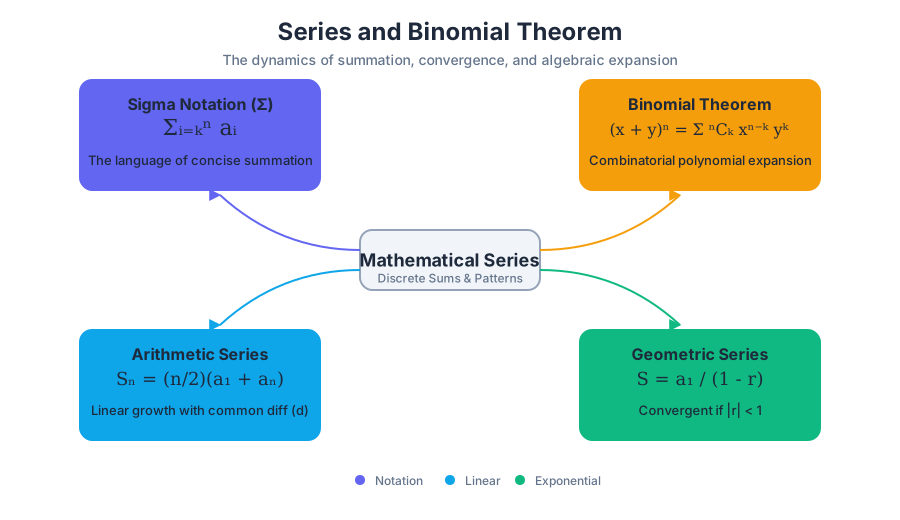
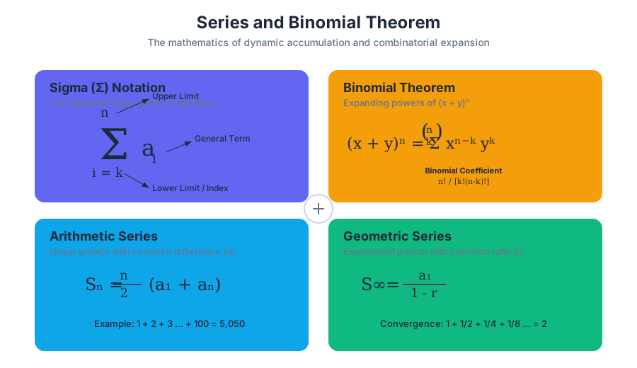
Limits and Continuity
Key concepts: Estimating limits from graphs · Algebraic limit properties · The Squeeze Theorem · Intermediate Value Theorem (IVT) · Continuity
Introduces the foundational concepts of calculus, defining how functions behave as they approach specific points or infinity.
Limits and Continuity
The study of calculus begins not with the derivative or the integral, but with the limit. If algebra is the study of fixed values and equations, calculus is the study of change—and the limit is the mathematical language used to describe how functions behave as they approach specific points or boundaries. Continuity, in turn, is the formalization of the intuitive idea of a "unbroken" curve. Together, these concepts provide the rigorous foundation upon which the entire edifice of modern analysis is built.
The Formal Definition of a Limit
At its core, a limit describes the value that a function $f(x)$ "approaches" as the input $x$ gets closer and closer to some value $c$. Crucially, the limit is concerned with the behavior of the function near $c$, not necessarily at $c$.
Formal Definition ($\epsilon-\delta$): We say that $\lim_{x \to c} f(x) = L$ if for every number $\epsilon > 0$, there exists a number $\delta > 0$ such that if $0 < |x - c| < \delta$, then $|f(x) - L| < \epsilon$.
This definition, pioneered by Cauchy and Weierstrass, transformed calculus from a collection of heuristic methods into a rigorous branch of mathematics. It essentially states that we can make $f(x)$ as close to $L$ as we like by making $x$ sufficiently close to $c$.
One-Sided Limits
In many cases, a function behaves differently depending on whether we approach $c$ from the left (values smaller than $c$) or the right (values larger than $c$).
- Left-hand limit: $\lim_{x \to c^-} f(x)$
- Right-hand limit: $\lim_{x \to c^2} f(x)$
A limit exists if and only if both one-sided limits exist and are equal: $$\lim_{x \to c} f(x) = L \iff \lim_{x \to c^-} f(x) = \lim_{x \to c^+} f(x) = L$$
Estimating Limits: Graphical and Numerical Approaches
Before applying algebraic rigor, we often estimate limits by observing trends.
Graphical Estimation
When looking at a graph, we trace the path of the function from both sides of $x = c$. If the "y-values" converge to a single height, that height is the limit.
- Holes (Removable Discontinuities): The limit exists even if the point is missing.
- Jumps: The left and right limits are different; the general limit does not exist (DNE).
- Vertical Asymptotes: The function grows without bound ($\infty$ or $-\infty$); the limit DNE (though we describe the direction of infinity).
Numerical Estimation
We can approximate a limit by evaluating the function at points increasingly close to $c$. For example, to find $\lim_{x \to 2} f(x)$, we might test $x = 1.9, 1.99, 1.999$ and $x = 2.1, 2.01, 2.001$.
| $x$ | $f(x) = \frac{x^2 - 4}{x - 2}$ | Observation |
|---|---|---|
| 1.9 | 3.9 | Approaching from left |
| 1.99 | 3.99 | Getting closer to 4 |
| 2.01 | 4.01 | Approaching from right |
| 2.001 | 4.001 | Getting closer to 4 |
| 2.0 | undefined | Point does not exist, but limit does |
Algebraic Limit Properties
Calculating limits by hand using the $\epsilon-\delta$ definition is cumbersome. Instead, we use Limit Laws, which allow us to break complex functions into simpler components.
The Limit Laws
Assume $\lim_{x \to c} f(x) = L$ and $\lim_{x \to c} g(x) = M$.
| Law Name | Formula |
|---|---|
| Sum/Difference | $\lim_{x \to c} [f(x) \pm g(x)] = L \pm M$ |
| Constant Multiple | $\lim_{x \to c} [k \cdot f(x)] = k \cdot L$ |
| Product | $\lim_{x \to c} [f(x) \cdot g(x)] = L \cdot M$ |
| Quotient | $\lim_{x \to c} \frac{f(x)}{g(x)} = \frac{L}{M}$, provided $M \neq 0$ |
| Power/Root | $\lim_{x \to c} [f(x)]^n = L^n$ |
Strategies for Indeterminate Forms
When direct substitution results in $0/0$ or $\infty/\infty$, the limit is in an indeterminate form. This does not mean the limit doesn't exist; it means more work is required.
- Factoring: For rational functions, factor the numerator and denominator to cancel the term causing the zero.
- Rationalization: For functions involving square roots, multiply by the conjugate.
- Trigonometric Identities: Use identities like $\lim_{\theta \to 0} \frac{\sin \theta}{\theta} = 1$ to simplify expressions.
# Implementation of a numerical limit estimator in Python
# This script evaluates a function progressively closer to a target 'c'
# to estimate the limit from both sides.

def f(x):
    # Example: (x^2 - 1) / (x - 1) -> Limit as x -> 1 is 2
    try:
        return (x**2 - 1) / (x - 1)
    except ZeroDivisionError:
        return float('nan')

def estimate_limit(func, c, tolerance=1e-9):
    steps = [0.1, 0.01, 0.001, 0.0001, 0.00001, 0.000001]

    print(f"{'Step':<10} | {'Left f(x)':<15} | {'Right f(x)':<15}")
    print("-" * 45)

    for s in steps:
        left_val = func(c - s)
        right_val = func(c + s)
        print(f"{s:<10} | {left_val:<15.7f} | {right_val:<15.7f}")

estimate_limit(f, 1.0)
The Squeeze Theorem
The Squeeze Theorem (also known as the Sandwich Theorem) is used to find the limit of a function that is difficult to evaluate directly by "trapping" it between two functions whose limits are known.
Theorem: If $g(x) \leq f(x) \leq h(x)$ for all $x$ in an open interval containing $c$ (except possibly at $c$), and if: $$\lim_{x \to c} g(x) = \lim_{x \to c} h(x) = L$$ then: $$\lim_{x \to c} f(x) = L$$
Classic Example: $x^2 \sin(1/x)$
Consider $\lim_{x \to 0} x^2 \sin(\frac{1}{x})$.
- We know that $-1 \leq \sin(\frac{1}{x}) \leq 1$ for all $x \neq 0$.
- Multiplying by $x^2$ (which is always $\geq 0$), we get: $-x^2 \leq x^2 \sin(\frac{1}{x}) \leq x^2$.
- Since $\lim_{x \to 0} (-x^2) = 0$ and $\lim_{x \to 0} (x^2) = 0$, by the Squeeze Theorem, $\lim_{x \to 0} x^2 \sin(\frac{1}{x}) = 0$.
Continuity
Continuity is the mathematical formalization of "smoothness." A function is continuous if you can draw its graph without lifting your pencil. However, for calculus, we need a point-specific definition.
The Three-Part Test for Continuity
A function $f(x)$ is continuous at a point $c$ if and only if:
- $f(c)$ is defined (the point exists).
- $\lim_{x \to c} f(x)$ exists (the left and right limits match).
- $\lim_{x \to c} f(x) = f(c)$ (the limit matches the actual value).
If any of these conditions fail, the function is discontinuous at $c$.
Types of Discontinuities
| Type | Description | Graphical Feature | Removable? |
|---|---|---|---|
| Removable | Limit exists, but $f(c)$ is either undefined or different. | A "hole" in the graph. | Yes (by redefining $f(c)$). |
| Jump | Left and right limits exist but are not equal. | A vertical break between segments. | No. |
| Infinite | Function approaches $\pm \infty$ as $x \to c$. | A vertical asymptote. | No. |
| Oscillating | Function oscillates infinitely fast as it nears $c$. | Dense "zig-zags" (e.g., $\sin(1/x)$). | No. |
/* Mathematical derivation of continuity for a piecewise function */
/* Objective: Find 'k' such that f(x) is continuous at x = 2 */

f(x) = {
  x^2 + k,  if x <= 2
  3x - 1,   if x > 2
}

Step 1: Find the left-hand limit as x -> 2
lim_{x -> 2-} f(x) = 2^2 + k = 4 + k

Step 2: Find the right-hand limit as x -> 2
lim_{x -> 2+} f(x) = 3(2) - 1 = 5

Step 3: Set limits equal for continuity
4 + k = 5
k = 1
The Intermediate Value Theorem (IVT)
The Intermediate Value Theorem is an "existence theorem." It doesn't tell you where a value is, but it guarantees that a value must exist under certain conditions.
Theorem: If $f$ is continuous on the closed interval $[a, b]$, and $N$ is any number between $f(a)$ and $f(b)$ (where $f(a) \neq f(b)$), then there exists at least one number $c$ in $(a, b)$ such that $f(c) = N$.
Why It Matters: Root Finding
The most common application of IVT is proving that a function has a root (a zero) in a given interval. If $f(a)$ is negative and $f(b)$ is positive, and $f$ is continuous, there must be some $c$ between $a$ and $b$ where $f(c) = 0$. This is the logic behind the Bisection Method used in computer science to solve equations.
Pitfall: Continuity is Mandatory
If a function is not continuous, the IVT does not apply. A step function can "jump" over the value $N$ without ever actually equaling it.
Infinite Limits and Asymptotes
Limits also describe the "end behavior" of functions or their behavior near singularities.
Vertical Asymptotes
If $f(x)$ approaches $\infty$ or $-\infty$ as $x$ approaches $c$ from either side, the line $x = c$ is a vertical asymptote. This typically occurs in rational functions when the denominator is zero and the numerator is non-zero.
Limits at Infinity (Horizontal Asymptotes)
We use $\lim_{x \to \infty} f(x)$ to describe what happens to a function as $x$ grows very large.
- If the limit is a finite number $L$, then $y = L$ is a horizontal asymptote.
- For rational functions $f(x) = \frac{P(x)}{Q(x)}$:
- If degree($P$) < degree($Q$), the limit is 0.
- If degree($P$) = degree($Q$), the limit is the ratio of leading coefficients.
- If degree($P$) > degree($Q$), the limit is $\pm \infty$ (slant or no horizontal asymptote).
// Real-world usage: A simple "Camera Smoothing" function in a
// game engine (like Unity or Three.js) using the concept of limits.
// As time progresses, the camera position approaches the target.

function smoothMove(currentPos, targetPos, lerpFactor) {
    /**
     * This is a discrete approximation of:
     * lim (t -> infinity) Position(t) = targetPos
     *
     * lerpFactor (0.1) means the camera moves 10% of the
     * remaining distance every frame.
     */
    return currentPos + (targetPos - currentPos) * lerpFactor;
}

// Usage in a game loop:
let cameraX = 0;
let playerX = 100;

function update() {
    cameraX = smoothMove(cameraX, playerX, 0.1);
    console.log(`Camera is at: ${cameraX.toFixed(2)}`);
    // Over time, cameraX approaches 100 but mathematically
    // only reaches it at the limit.
}
Common Pitfalls and Misconceptions
- Confusing $f(c)$ with the Limit: Students often think that if $f(c)$ is undefined, the limit doesn't exist. Remember: the limit is about the neighborhood, not the point.
- Assuming $0/0$ is Zero or One: $0/0$ is an indeterminate form. It could be $5, -2, \infty$, or not exist at all. You must use algebraic manipulation.
- Ignoring One-Sided Limits: For piecewise functions or functions with absolute values, you must check both sides. If they don't match, the general limit DNE.
- Misapplying IVT: Forgetting to check if the function is continuous on the entire closed interval. A single point of discontinuity between $a$ and $b$ invalidates the theorem.
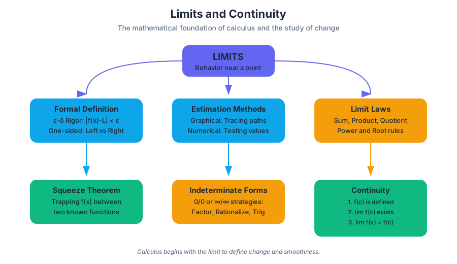
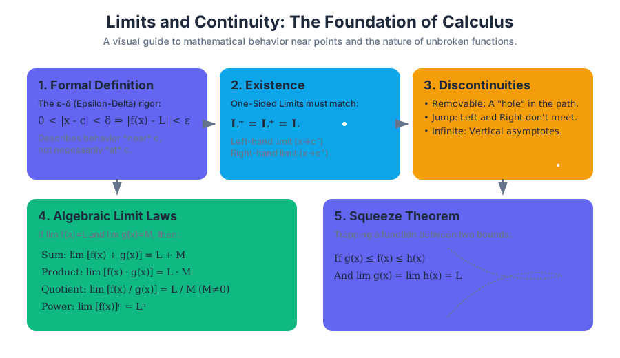
Precalculus Course Challenge
Key concepts: Mastery points · Skills assessment · Comprehensive review
A comprehensive 30-question assessment to evaluate mastery of all precalculus skills covered in the course.
Precalculus Course Challenge
The Precalculus Course Challenge represents the capstone assessment of the Precalculus curriculum, a rigorous synthesis of algebraic sophistication, trigonometric depth, and an introduction to the discrete structures of linear algebra. Unlike unit-specific tests, the Course Challenge is a stochastic sampling of the entire domain, designed to evaluate a student's Mastery Points—a quantitative metric of their proficiency across hundreds of distinct mathematical skills.
In a modern pedagogical framework, this challenge is not merely a "final exam" but a diagnostic engine. It utilizes adaptive sequencing to identify gaps in a student's mental model of functions, vectors, and complex systems. To succeed, one must move beyond rote memorization of identities and develop a high-level architectural understanding of how different mathematical objects—such as matrices and trigonometric functions—interact to model the physical world.
The Architecture of Mastery
The challenge is built upon a Skills Assessment framework. Every problem solved correctly contributes to the total mastery score of the course, which typically aggregates thousands of points across various units.
Technical Prerequisites and Environment
From a systems perspective, the Course Challenge is an interactive web application. The source material emphasizes a critical technical requirement: JavaScript must be enabled. This is because the assessment engine relies on client-side logic for several high-stakes operations:
- State Management: Tracking progress through the 30-question set without requiring a full page reload for every interaction.
- Dynamic Rendering: Utilizing libraries (often MathJax or KaTeX) to render complex LaTeX-based mathematical notation in real-time.
- Interactive Graphing: Providing embedded tools (such as Desmos-style calculators) that allow students to visualize rational functions or conic sections.
- Input Validation: Real-time checking of syntax for algebraic expressions to ensure that a student is penalized for mathematical errors, not formatting mistakes.
Core Competencies and Exam Patterns
The Course Challenge samples from ten primary units. To achieve a 100% mastery score, a student must demonstrate "Proficient" or "Mastered" status in each of the following domains.
1. Composite and Inverse Functions
This unit transitions students from thinking about functions as static equations to thinking about them as transformative operators. The primary challenge lies in Domain Restriction; many functions (like $x^2$ or $\sin(x)$) are not inherently invertible unless their domain is strictly limited to ensure they are one-to-one (injective).
Theorem: The Horizontal Line Test A function $f$ has an inverse $f^{-1}$ if and only if no horizontal line intersects the graph of $f$ at more than one point. This is the geometric equivalent of the algebraic requirement for a function to be injective.
| Concept | Mathematical Representation | Key Requirement |
|---|---|---|
| Composition | $(f \circ g)(x) = f(g(x))$ | Range of $g$ must be subset of Domain of $f$ |
| Invertibility | $f(f^{-1}(x)) = x$ | Function must be monotonic on the interval |
| Verification | $f(g(x)) = x$ AND $g(f(x)) = x$ | Both directions must hold for $g = f^{-1}$ |
2. Trigonometry and Sinusoidal Modeling
Trigonometry in Precalculus moves beyond right-triangle geometry into the realm of periodic oscillations. The Course Challenge frequently tests the ability to model real-world phenomena (tides, sound waves, ferris wheels) using the general sinusoidal form: $$y = A \sin(B(x - C)) + D$$
Where:
- $A$ is the Amplitude (vertical stretch).
- $B$ determines the Period ($P = \frac{2\pi}{B}$).
- $C$ is the Phase Shift (horizontal translation).
- $D$ is the Midline (vertical shift).
3. Rational Functions and Asymptotic Behavior
Rational functions, defined as $R(x) = \frac{P(x)}{Q(x)}$ where $P$ and $Q$ are polynomials, introduce the concept of limits without formalizing the calculus notation. Students must identify:
- Vertical Asymptotes: Where the denominator $Q(x) = 0$ (and $P(x) \neq 0$).
- Removable Discontinuities (Holes): Where both $P(x)$ and $Q(x)$ share a common factor.
- End Behavior: Determined by the ratio of the leading coefficients if the degrees of $P$ and $Q$ are equal.
| Degree Comparison | Asymptote Type | Behavior |
|---|---|---|
| $deg(P) < deg(Q)$ | Horizontal | $y = 0$ (x-axis) |
| $deg(P) = deg(Q)$ | Horizontal | $y = \frac{a_n}{b_n}$ (ratio of leading coefficients) |
| $deg(P) = deg(Q) + 1$ | Slant (Oblique) | Found via polynomial long division |
| $deg(P) > deg(Q) + 1$ | Non-linear | Function grows quadratically, cubically, etc. |
Advanced Computational Structures: Vectors and Matrices
A significant portion of the Course Challenge focuses on linear algebra. This is where Precalculus becomes "pre-physics" and "pre-engineering."
Vectors: Magnitude and Direction
Vectors are treated both geometrically (arrows in space) and analytically (ordered pairs or triples). The challenge tests the conversion between Rectangular Form $\langle x, y \rangle$ and Polar Form $(r, \theta)$.
import math

def vector_to_polar(x, y):
    """
    Converts a 2D vector from rectangular coordinates to polar form.
    Returns (magnitude, angle_in_radians).
    """
    magnitude = math.sqrt(x**2 + y**2)
    # atan2 handles quadrant logic automatically
    angle = math.atan2(y, x)

    return magnitude, angle

# Example: Vector <3, 4>
mag, ang = vector_to_polar(3, 4)
print(f"Magnitude: {mag}, Angle: {ang:.4f} rad")
# Output: Magnitude: 5.0, Angle: 0.9273 rad
Matrices: Transformations and Systems
Matrices are presented as tools for solving systems of linear equations and performing geometric transformations (rotations, scaling, reflections). The Determinant ($\det(A)$) is a critical value; if $\det(A) = 0$, the matrix is singular (non-invertible), representing a transformation that collapses a dimension.
\text{For a } 2 \times 2 \text{ matrix } A = \begin{pmatrix} a & b \\ c & d \end{pmatrix}:
\\
\det(A) = ad - bc
\\
A^{-1} = \frac{1}{ad - bc} \begin{pmatrix} d & -b \\ -c & a \end{pmatrix}
Conic Sections: The Geometry of Algebra
The Course Challenge requires students to identify and graph parabolas, circles, ellipses, and hyperbolas from their general second-degree equations.
$$Ax^2 + Bxy + Cy^2 + Dx + Ey + F = 0$$
The focus is usually on the standard forms, which allow for the immediate identification of the center $(h, k)$ and the lengths of the major/minor axes.
| Conic Section | Standard Equation (Horizontal) | Key Features |
|---|---|---|
| Circle | $(x-h)^2 + (y-k)^2 = r^2$ | Constant radius $r$ |
| Ellipse | $\frac{(x-h)^2}{a^2} + \frac{(y-k)^2}{b^2} = 1$ | Foci at $c^2 = a^2 - b^2$ |
| Hyperbola | $\frac{(x-h)^2}{a^2} - \frac{(y-k)^2}{b^2} = 1$ | Asymptotes: $y - k = \pm \frac{b}{a}(x - h)$ |
| Parabola | $(x-h)^2 = 4p(y-k)$ | Focus at $(h, k+p)$, Directrix at $y = k-p$ |
Complex Numbers and Polar Form
The Course Challenge bridges algebra and trigonometry through the complex plane. Every complex number $z = a + bi$ can be represented as $z = r(\cos \theta + i \sin \theta)$, or more elegantly using Euler's formula: $z = re^{i\theta}$.
This representation simplifies the multiplication and division of complex numbers:
- Multiplication: Multiply magnitudes, add angles.
- Division: Divide magnitudes, subtract angles.
- De Moivre's Theorem: $(r(\cos \theta + i \sin \theta))^n = r^n(\cos(n\theta) + i \sin(n\theta))$.
Strategy for the 30-Question Challenge
The Course Challenge is a marathon, not a sprint. Because it samples from the entire 10-unit curriculum, a student may encounter a question on matrix multiplication followed immediately by one on trigonometric identities.
Common Exam Patterns
- The "Reverse" Problem: Instead of giving you a function and asking for the graph, the exam provides a graph and asks for the equation. This requires identifying key features (asymptotes, intercepts, periods) and working backward.
- The Multi-Step Identity: Using angle addition formulas to find exact values for non-standard angles (e.g., $\sin(75^\circ)$ using $45^\circ + 30^\circ$).
- Vector Word Problems: Calculating the resultant velocity of an airplane flying in a crosswind. This requires breaking vectors into components, adding them, and converting back to polar form.
Implementation of a Mastery Tracking System
In a production-grade educational platform, the mastery state is often managed via a structured database schema. This allows the system to determine which questions to serve next based on the student's current "Level" (Attempted, Familiar, Proficient, Mastered).
-- Conceptual schema for tracking Course Challenge progress
CREATE TABLE student_mastery (
    student_id UUID REFERENCES users(id),
    skill_id VARCHAR(255) PRIMARY KEY,
    mastery_points INT DEFAULT 0, -- 0 to 100
    last_attempt TIMESTAMP,
    status ENUM('not_started', 'familiar', 'proficient', 'mastered')
);

CREATE TABLE challenge_sessions (
    session_id UUID PRIMARY KEY,
    student_id UUID REFERENCES users(id),
    score_percentage DECIMAL(5,2),
    questions_answered INT,
    completed_at TIMESTAMP
);
Common Pitfalls to Avoid
- Radians vs. Degrees: This is the most frequent source of error in the Trigonometry units. Always check the mode of the calculator and the units specified in the problem.
- The Ambiguous Case (SSA): When using the Law of Sines to solve a triangle, remember that there may be zero, one, or two possible triangles depending on the given side lengths and angle.
- Matrix Multiplication Order: Matrix multiplication is not commutative ($AB \neq BA$). The order of transformations matters.
- Asymptote vs. Hole: Forgetting to simplify a rational expression before identifying vertical asymptotes often leads to identifying a "hole" as an asymptote.
Insight: The Power of Limits While Precalculus avoids the formal definition of a derivative, the Course Challenge tests the "Limit" concept through end behavior. Understanding that $\frac{1}{x} \to 0$ as $x \to \infty$ is the fundamental intuition required for all of Calculus.
Practical Application: Modeling with Functions
A senior engineer might use these concepts to model the load on a bridge or the signal processing in a wireless network. For example, a mixture problem (Unit 3: Rational Functions) can be modeled as: $$C(t) = \frac{\text{Amount of Solute}}{\text{Total Volume of Solution}}$$ As $t \to \infty$, the concentration $C(t)$ approaches the concentration of the incoming stream—a horizontal asymptote in action.
// Example of a client-side validation for a rational function input
// This illustrates why JavaScript is required for the Course Challenge.

function validateRationalFunction(numerator, denominator, xValue) {
    try {
        const numVal = eval(numerator.replace(/x/g, `(${xValue})`));
        const denVal = eval(denominator.replace(/x/g, `(${xValue})`));

        if (denVal === 0) {
            return { status: "undefined", type: "Vertical Asymptote or Hole" };
        }
        return { status: "defined", value: numVal / denVal };
    } catch (error) {
        return { status: "error", message: "Invalid mathematical syntax" };
    }
}

console.log(validateRationalFunction("x + 2", "x - 3", 3));
// Output: { status: "undefined", type: "Vertical Asymptote or Hole" }
Summary of Mastery Points
The Course Challenge is the ultimate test of mathematical "fluidity." It requires the student to switch contexts rapidly—from the geometric properties of an ellipse to the algebraic manipulation of a complex conjugate. By the end of the challenge, a student who has achieved mastery is not just ready for Calculus; they have developed a robust toolkit for analyzing any system that can be described by a function.
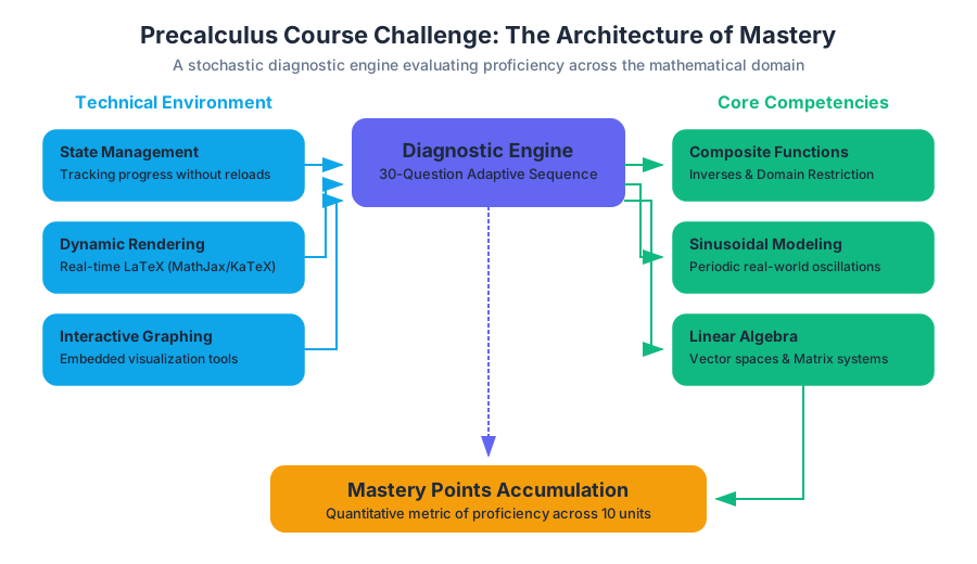
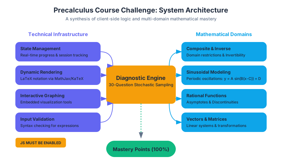
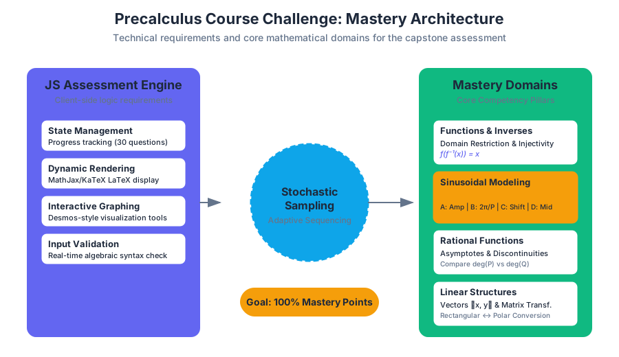
Source Materials
Study Precalculus with AI — Free on Lykke
Sign up for free to generate personalized flashcards, quizzes, and study guides from this course. Chat with an AI tutor that knows the material.
Get Started FreeView this course wiki on Lykke · Browse all public course wikis