Precalculus 2e

Functions and Linear Modeling

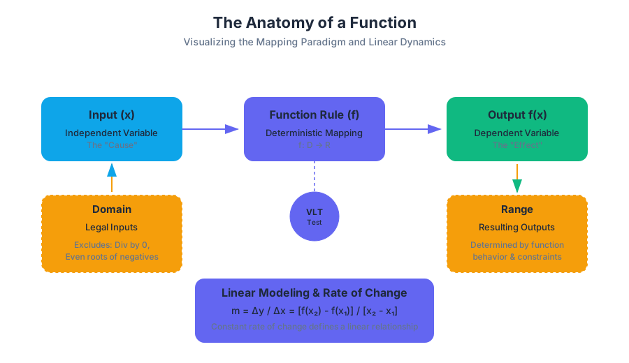
In the hierarchy of mathematical analysis, the function serves as the fundamental unit of mapping. It is the formalization of "relationship"—a deterministic rule that assigns each element from a set of inputs to exactly one element in a set of outputs. While elementary algebra treats equations as static balances to be solved, precalculus shifts the perspective toward functional analysis, where we examine how change in one variable propagates through a system to affect another.

This section explores the mechanics of functions, the constraints of their domains, the dynamics of their rates of change, and the foundational application of Linear Modeling. By mastering these concepts, we move from solving for $x$ to understanding the behavior of $f(x)$.

Function Notation and the Mapping Paradigm

At its core, a function is a specialized type of relation. While all functions are relations, not all relations are functions. The distinguishing characteristic is the uniqueness of the output.

Definition: The Function A function $f$ is a relation that assigns to each element $x$ in a set $D$ (the domain) exactly one element $y$ in a set $R$ (the range). This is notationally represented as $f: D \to R$.

The transition to Function Notation ($f(x)$) is often the first hurdle for students. It is crucial to view $f(x)$ not as "f times x," but as "the value of the output $f$ when the input is $x$." This notation allows for the clear expression of complex operations, such as composition and transformation, which are cumbersome in $y = \dots$ format.

The Vertical Line Test (VLT)

In a Cartesian coordinate system, a relation is a function if and only if no vertical line intersects its graph more than once. This is the visual manifestation of the "one output per input" rule. If a vertical line hits two points, the same $x$ has two different $y$ values, violating the definition of a function.

Evaluating and Simplifying Functions

Evaluating a function involves substituting a specific value or expression into every instance of the independent variable. This often requires algebraic manipulation, particularly when dealing with difference quotients or composite expressions.

Concept	Notation	Description
Input	$x$	The independent variable; the "cause."
Output	$f(x)$	The dependent variable; the "effect."
Rule	$f$	The specific mapping or algorithm applied to $x$.
Mapping	$x \mapsto f(x)$	The process of transforming input to output.

# A robust implementation of a mathematical function evaluator in Python.
# This demonstrates function mapping with domain validation.

import math

class MathematicalFunction:
    def __init__(self, name, rule, domain_check=None):
        self.name = name
        self.rule = rule
        self.domain_check = domain_check

    def evaluate(self, x):
        """Evaluates f(x) with explicit domain validation."""
        if self.domain_check and not self.domain_check(x):
            raise ValueError(f"Input {x} is outside the domain of {self.name}")
        return self.rule(x)

# Example: f(x) = sqrt(x - 5)
# Domain: [5, infinity)
f = MathematicalFunction(
    name="f(x) = sqrt(x - 5)",
    rule=lambda x: math.sqrt(x - 5),
    domain_check=lambda x: x >= 5
)

try:
    print(f"f(9) = {f.evaluate(9)}")   # Output: 2.0
    print(f"f(4) = {f.evaluate(4)}")   # Raises ValueError
except ValueError as e:
    print(e)

Domain and Range: The Constraints of Reality

The Domain of a function is the set of all possible "legal" inputs. In pure mathematics, the domain is restricted by the algebraic properties of the real numbers. In applied modeling, the domain is further restricted by the physical or logical constraints of the problem.

Algebraic Restrictions

There are two primary "sins" in real-numbered algebra that define the domain of most functions:

1. Division by Zero: Any input that results in a zero denominator must be excluded.
2. Even Roots of Negative Numbers: In the real number system, the radicand of an even-indexed root must be non-negative ($\geq 0$).

Interval Notation

To describe these sets efficiently, we use Interval Notation. This system uses brackets [] for inclusive boundaries (where the endpoint is part of the set) and parentheses () for exclusive boundaries.

Set Description	Inequality	Interval Notation
Values between $a$ and $b$, inclusive	$a \le x \le b$	$[a, b]$
Values greater than $a$	$x > a$	$(a, \infty)$
All real numbers except $c$	$x \neq c$	$(-\infty, c) \cup (c, \infty)$
Values less than or equal to $b$	$x \le b$	$(-\infty, b]$

The Range is the set of all possible output values. While the domain is often found by looking for what $x$ cannot be, the range is often found by observing the behavior of the function (e.g., the minimum value of a parabola or the horizontal asymptote of a rational function).

Rates of Change: The Dynamics of Functions

A function describes a state, but the Rate of Change describes the motion between states. This concept is the conceptual bridge to the Derivative in Calculus.

Average Rate of Change (AROC)

The average rate of change of a function $f$ over an interval $[x_1, x_2]$ is the ratio of the change in the output values to the change in the input values. Geometrically, this is the slope of the secant line connecting two points on the graph.

$$AROC = \frac{\Delta y}{\Delta x} = \frac{f(x_2) - f(x_1)}{x_2 - x_1}$$

The Difference Quotient

To find the rate of change at a specific point (the instantaneous rate of change), we use the Difference Quotient. This formula calculates the average rate of change between a point $x$ and a point slightly further away, $x+h$.

\text{Difference Quotient} = \frac{f(x + h) - f(x)}{h}, \quad h \neq 0

In Calculus, we take the limit as $h$ approaches zero to find the derivative. In Precalculus, we focus on the algebraic simplification of this expression, which is a critical skill for future success in analysis.

Worked Example: Difference Quotient

For $f(x) = x^2 + 3x$:

1. $f(x+h) = (x+h)^2 + 3(x+h) = x^2 + 2xh + h^2 + 3x + 3h$
2. $f(x+h) - f(x) = (x^2 + 2xh + h^2 + 3x + 3h) - (x^2 + 3x) = 2xh + h^2 + 3h$
3. $\frac{2xh + h^2 + 3h}{h} = 2x + h + 3$

As $h \to 0$, the rate of change becomes $2x + 3$.

Linear Functions and Modeling

A Linear Function is a function with a constant rate of change. This is the simplest form of modeling, where the output changes by a fixed amount for every unit increase in the input.

Forms of Linear Equations

Different contexts require different algebraic representations of lines.

Form	Equation	Primary Use Case
Slope-Intercept	$f(x) = mx + b$	Graphing and identifying the starting value ($b$).
Point-Slope	$y - y_1 = m(x - x_1)$	Constructing a model from a known point and rate.
General Form	$Ax + By = C$	Analyzing intercepts and linear programming.

Modeling Real-World Data

Linear modeling involves identifying the initial value (the y-intercept) and the constant rate (the slope).

Example: Telecommunications Pricing A data plan costs $30 per month plus $5 per gigabyte of data used. Here, $b = 30$ (fixed cost) and $m = 5$ (variable rate). The model is $C(g) = 5g + 30$.

Linear Regression

When data points do not fall perfectly on a line, we use Linear Regression to find the "Line of Best Fit." This minimizes the sum of the squares of the vertical deviations (residuals) between the data points and the line.

-- Conceptual SQL query for calculating the slope (m) and intercept (b) 
-- of a linear regression line from a dataset of (x, y) coordinates.
-- Uses the standard Least Squares formulas.

SELECT 
    (count(*) * sum(x*y) - sum(x) * sum(y)) / 
    (count(*) * sum(x*x) - sum(x) * sum(x)) AS slope_m,
    
    (sum(y) - ((count(*) * sum(x*y) - sum(x) * sum(y)) / 
    (count(*) * sum(x*x) - sum(x) * sum(x))) * sum(x)) / 
    count(*) AS intercept_b
FROM sensor_readings;

Linear Transformations: Manipulating Function Geometry

Transformations allow us to create a family of functions based on a "parent" function. By applying constants to the input or output, we can shift, scale, or reflect the graph.

Vertical and Horizontal Shifts

• Vertical Shift: $g(x) = f(x) + k$. If $k > 0$, the graph moves up; if $k < 0$, it moves down.
• Horizontal Shift: $g(x) = f(x - h)$. If $h > 0$, the graph moves right; if $h < 0$, it moves left. (Note the subtraction in the formula).

Scaling and Reflections

• Vertical Stretch/Compression: $g(x) = a f(x)$. If $|a| > 1$, it stretches; if $0 < |a| < 1$, it compresses.
• Horizontal Stretch/Compression: $g(x) = f(bx)$. If $|b| > 1$, it compresses horizontally; if $0 < |b| < 1$, it stretches horizontally.
• Reflections: $-f(x)$ reflects across the x-axis; $f(-x)$ reflects across the y-axis.

Summary of Transformations

Operation	Transformation	Effect on $(x, y)$
$f(x) + k$	Vertical Shift	$(x, y + k)$
$f(x - h)$	Horizontal Shift	$(x + h, y)$
$a f(x)$	Vertical Scale	$(x, ay)$
$f(bx)$	Horizontal Scale	$(x/b, y)$
$-f(x)$	Reflection (x-axis)	$(x, -y)$
$f(-x)$	Reflection (y-axis)	$(-x, y)$

/**
 * A utility to calculate transformed coordinates.
 * Demonstrates the mathematical application of transformations.
 */
interface Point {
    x: number;
    y: number;
}

class FunctionTransformer {
    // Represents g(x) = a * f(b(x - h)) + k
    constructor(
        private a: number = 1, // Vertical Scale
        private b: number = 1, // Horizontal Scale
        private h: number = 0, // Horizontal Shift
        private k: number = 0  // Vertical Shift
    ) {}

    transformPoint(p: Point): Point {
        return {
            // Horizontal: x_new = (x_old / b) + h
            x: (p.x / this.b) + this.h,
            // Vertical: y_new = (a * y_old) + k
            y: (this.a * p.y) + this.k
        };
    }
}

const myTransform = new FunctionTransformer(2, 1, 5, -10); 
// Stretch vertically by 2, shift right 5, shift down 10
console.log(myTransform.transformPoint({x: 0, y: 0})); // {x: 5, y: -10}

Common Pitfalls and Edge Cases

1. Confusing $f(x+h)$ with $f(x)+h$: The former is a horizontal shift (input modification), while the latter is a vertical shift (output modification).
2. Order of Transformations: When multiple transformations are applied, the order matters. Generally, follow the order of operations: perform horizontal shifts, then horizontal scaling, then reflections, then vertical scaling, and finally vertical shifts.
3. Domain of Composite Functions: The domain of $f(g(x))$ is not just the domain of the final simplified expression. It must also exclude any values that are not in the domain of the inner function $g(x)$.
4. Slope of Vertical Lines: A vertical line has an "undefined" slope because $\Delta x = 0$. Consequently, vertical lines are not functions of $x$.

# Using gnuplot to visualize the difference between 
# f(x) = x^2 and its transformation g(x) = 2(x-3)^2 + 5

# Define functions
f(x) = x**2
g(x) = 2 * (x - 3)**2 + 5

# Set plot parameters
set terminal png size 800,600
set output 'transformation_plot.png'
set grid
set xrange [-5:10]
set yrange [-5:30]

# Plot
plot f(x) title 'Parent: f(x)=x^2' lw 2, \
     g(x) title 'Transformed: g(x)=2(x-3)^2+5' lw 2

Polynomial and Rational Functions

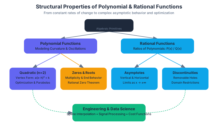
The transition from linear modeling to polynomial and rational functions marks a critical juncture in mathematical maturity. While linear functions describe constant rates of change, Polynomial Functions allow for the modeling of acceleration, curvature, and complex oscillations. Rational Functions, defined as the ratio of two polynomials, introduce the concept of asymptotic behavior and discontinuities—concepts that form the bedrock of calculus and complex analysis.

In the context of modern engineering and data science, these functions are not merely abstract constructs; they are the primitives used in spline interpolation, signal processing, and the optimization of cost functions. This article explores the structural properties, behavior, and algebraic foundations of these function families.

Quadratic Functions and Optimization

A Quadratic Function is a polynomial function of degree 2. Its graph is a parabola, a symmetrical curve that represents the simplest non-linear relationship where the rate of change is itself changing at a constant rate.

1. Definitions and Forms

The utility of a quadratic function often depends on the algebraic form in which it is expressed.

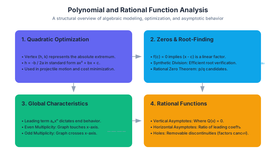
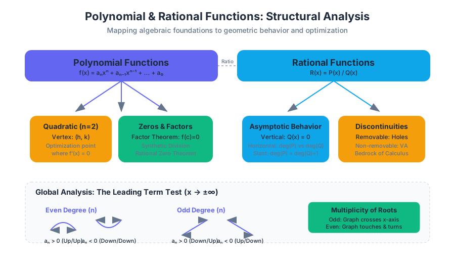
The Vertex Form: $f(x) = a(x - h)^2 + k$ This form is computationally superior for identifying the Vertex $(h, k)$, which represents the absolute maximum or minimum of the function. The value of $a$ determines the "stretch" and the direction of the opening (upward if $a > 0$, downward if $a > 0$).

2. Mechanics of the Vertex

The vertex is the critical point where the function's derivative is zero. In the standard form $f(x) = ax^2 + bx + c$, the x-coordinate of the vertex is derived via $h = -b / (2a)$. Substituting $h$ back into the function yields the y-coordinate $k$.

Feature	General Form: $ax^2 + bx + c$	Vertex Form: $a(x-h)^2 + k$
Y-Intercept	$(0, c)$	Found by calculating $f(0)$
Vertex	$(-b/2a, f(-b/2a))$	$(h, k)$
Axis of Symmetry	$x = -b/2a$	$x = h$
Optimization	Requires calculation	Immediately visible

3. Implementation: Finding the Extreme Value

In engineering, finding the vertex is synonymous with optimization—minimizing material use or maximizing projectile range.

import numpy as np

def analyze_quadratic(a, b, c):
    """
    Analyzes a quadratic function f(x) = ax^2 + bx + c.
    Returns the vertex, roots (real or complex), and the nature of the extremum.
    """
    # Calculate the vertex (h, k)
    h = -b / (2 * a)
    k = a * (h**2) + b * h + c
    
    # Calculate the discriminant
    discriminant = b**2 - 4 * a * c
    
    # Solve for roots using the quadratic formula
    if discriminant >= 0:
        roots = ((-b + np.sqrt(discriminant)) / (2 * a), 
                 (-b - np.sqrt(discriminant)) / (2 * a))
    else:
        roots = (complex(-b / (2 * a), np.sqrt(-discriminant) / (2 * a)),
                 complex(-b / (2 * a), -np.sqrt(-discriminant) / (2 * a)))
                 
    return {
        "vertex": (h, k),
        "type": "minimum" if a > 0 else "maximum",
        "roots": roots,
        "discriminant": discriminant
    }

# Example: Optimization of a revenue function R(p) = -2p^2 + 400p
result = analyze_quadratic(-2, 400, 0)
print(f"Optimal Price: {result['vertex'][0]}, Max Revenue: {result['vertex'][1]}")

---

Zeros of Polynomial Functions

As we move to higher-degree polynomials ($n > 2$), the complexity of finding zeros (or roots) increases. A zero of a function $f$ is a value $c$ such that $f(c) = 0$.

1. The Remainder and Factor Theorems

These theorems bridge the gap between polynomial division and function evaluation.

• Remainder Theorem: If a polynomial $f(x)$ is divided by $(x - c)$, the remainder is the value $f(c)$.
• Factor Theorem: A polynomial $f(x)$ has a factor $(x - c)$ if and only if $f(c) = 0$.

2. The Rational Zero Theorem

For a polynomial with integer coefficients, any rational zero must be of the form $p/q$, where $p$ is a factor of the constant term and $q$ is a factor of the leading coefficient. This significantly narrows the search space for roots in high-degree equations.

3. Synthetic Division: The Algorithm

Synthetic division is a shorthand method of polynomial division, specifically for the case of dividing by a linear factor $(x - c)$. It is computationally efficient and forms the basis for many root-finding algorithms.

ALGORITHM: Synthetic Division of P(x) by (x - c)
-----------------------------------------------
Input: Coefficients of P(x) = [a_n, a_{n-1}, ..., a_0], constant c
Output: Quotient coefficients [q_{n-1}, ..., q_0], Remainder r

1. Let current_val = a_n
2. Store a_n as the first coefficient of the quotient.
3. For i from n-1 down to 0:
    a. Multiply current_val by c.
    b. Add result to a_i.
    c. current_val = result + a_i
    d. If i > 0, store current_val as next quotient coefficient.
    e. If i == 0, current_val is the Remainder.

4. End Behavior and Multiplicity

The global shape of a polynomial is dictated by its Leading Term $a_n x^n$. As $x \to \pm \infty$, the leading term dominates all other terms.

Degree ($n$)	Leading Coeff ($a_n$)	Left Behavior ($x \to -\infty$)	Right Behavior ($x \to \infty$)
Even	Positive (+)	$f(x) \to \infty$	$f(x) \to \infty$
Even	Negative (-)	$f(x) \to -\infty$	$f(x) \to -\infty$
Odd	Positive (+)	$f(x) \to -\infty$	$f(x) \to \infty$
Odd	Negative (-)	$f(x) \to \infty$	$f(x) \to -\infty$

Multiplicity refers to how many times a specific factor $(x - c)$ is repeated. If the multiplicity is even, the graph "touches" the x-axis and turns around. If odd, the graph crosses the x-axis.

---

Rational Functions and Asymptotic Analysis

A Rational Function is defined as $f(x) = \frac{P(x)}{Q(x)}$, where $P$ and $Q$ are polynomials. These functions introduce "breaks" in the graph where the denominator $Q(x) = 0$.

1. Vertical Asymptotes and Holes

A rational function is undefined when $Q(x) = 0$. However, the nature of this undefined point depends on whether the factor also exists in the numerator.

• Vertical Asymptote: Occurs at $x = c$ if $Q(c) = 0$ and the factor $(x - c)$ does not cancel out with a factor in $P(x)$. The function approaches $\pm \infty$ as it nears $c$.
• Removable Discontinuity (Hole): Occurs at $x = c$ if the factor $(x - c)$ cancels out between $P(x)$ and $Q(x)$. The graph looks continuous except for a single missing point.

2. Horizontal and Slant Asymptotes

Horizontal asymptotes describe the End Behavior of the rational function. They are determined by comparing the degree of the numerator ($n$) to the degree of the denominator ($m$).

Condition	Asymptote Location	Description
$n < m$	$y = 0$	The x-axis is the horizontal asymptote.
$n = m$	$y = a_n / b_m$	The ratio of leading coefficients.
$n = m + 1$	Slant (Oblique)	Found using long division; $y = \text{quotient}$.
$n > m + 1$	No Horizontal/Slant	The function behaves like a polynomial of degree $n-m$.

3. Real-World Usage: Modeling Concentration

Rational functions are frequently used to model concentrations in a mixture over time.

# Using a CLI tool like 'gnuplot' to visualize a rational function
# Function: f(x) = (2x^2 - 2) / (x^2 - 4)
# This has vertical asymptotes at x = 2, x = -2 and a horizontal at y = 2

gnuplot -e "set terminal png; \
            set output 'rational_plot.png'; \
            set xrange [-10:10]; \
            set yrange [-10:10]; \
            set style line 1 lc rgb '#ad81ff' lt 1 lw 2; \
            plot (2*x**2 - 2)/(x**2 - 4) ls 1 title 'f(x) = (2x^2-2)/(x^2-4)';"

---

Inverses and Domain Restriction

An Inverse Function $f^{-1}(x)$ "reverses" the operation of $f(x)$. For an inverse to exist as a function, the original function must be One-to-One (passing the Horizontal Line Test).

1. Restricting the Domain

Most polynomials (like $f(x) = x^2$) are not one-to-one. To find an inverse, we must restrict the domain. For $f(x) = x^2$, we typically restrict $x \geq 0$, allowing the inverse $f^{-1}(x) = \sqrt{x}$ to exist.

2. Algebraic Method for Inverses

1. Replace $f(x)$ with $y$.
2. Interchange $x$ and $y$.
3. Solve for $y$.
4. Replace $y$ with $f^{-1}(x)$.

3. Complexity in Rational Inverses

Finding the inverse of a rational function often requires cross-multiplication and factoring to isolate the variable.

// A Rust representation of a Rational Function structure
// capable of basic evaluation and potentially symbolic inversion.

struct RationalFunction {
    numerator: Vec<f64>,   // Coefficients [a_0, a_1, ..., a_n]
    denominator: Vec<f64>, // Coefficients [b_0, b_1, ..., b_m]
}

impl RationalFunction {
    fn evaluate(&self, x: f64) -> Option<f64> {
        let num_val: f64 = self.numerator.iter().enumerate()
            .map(|(i, &coeff)| coeff * x.powi(i as i32)).sum();
        
        let den_val: f64 = self.denominator.iter().enumerate()
            .map(|(i, &coeff)| coeff * x.powi(i as i32)).sum();

        if den_val == 0.0 {
            None // Vertical Asymptote or Hole
        } else {
            Some(num_val / den_val)
        }
    }
}

fn main() {
    let f = RationalFunction {
        numerator: vec![-1.0, 0.0, 1.0],   // x^2 - 1
        denominator: vec![-4.0, 0.0, 1.0], // x^2 - 4
    };
    
    match f.evaluate(3.0) {
        Some(val) => println!("f(3) = {}", val),
        None => println!("Undefined at x=3"),
    }
}

---

Common Pitfalls and Misconceptions

Understanding these functions requires avoiding several "traps" that even advanced students fall into.

Pitfall	Explanation	Correction
Canceling Factors	Assuming a canceled factor $(x-c)$ means the function is defined at $c$.	A canceled factor creates a hole, not a point of continuity.
Asymptote Crossing	Believing a graph can never cross a horizontal asymptote.	Graphs can cross horizontal asymptotes in the short term; the asymptote only dictates behavior as $x \to \infty$.
Leading Term Neglect	Forgetting the sign of the leading coefficient in end behavior.	Always check the sign; a negative $a_n$ flips the entire graph vertically.
Complex Roots	Ignoring complex roots because they don't appear on the x-axis.	Complex roots are essential for the Fundamental Theorem of Algebra, which states a degree $n$ polynomial has $n$ roots.

Summary of the DEI Framework in Precalculus

In alignment with the OpenStax Precalculus 2e philosophy, the study of these functions is presented through a lens of accessibility and diverse representation. By using real-world examples that span various industries—from environmental science (modeling pollutant decay with rational functions) to social science (modeling population growth with polynomials)—the curriculum ensures that the mathematical concepts are grounded in a global context. This approach reduces barriers to entry in STEM by demonstrating the universal utility of algebraic modeling.

Exponential and Logarithmic Functions

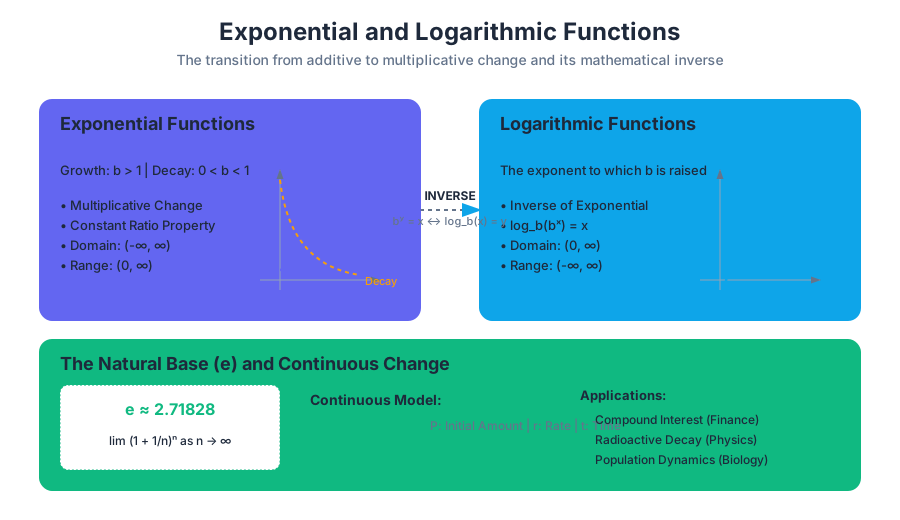
Exponential and logarithmic functions represent a fundamental shift in mathematical modeling, moving from additive change (linear functions) to multiplicative change. While linear models describe systems that grow by a constant amount per unit of time, exponential models describe systems where the rate of change is proportional to the current value. This characteristic makes them the primary language for describing biological growth, financial interest, radioactive decay, and information theory.

1. Foundations of Exponential Growth

An exponential function is a function of the form $f(x) = ab^x$, where $a$ is a non-zero constant (the initial value), $b$ is a positive real number not equal to 1 (the base), and $x$ is any real number. Unlike power functions (e.g., $x^2$), where the base is the variable, exponential functions place the variable in the exponent.

1.1 Growth vs. Decay

The behavior of the function is dictated by the base $b$. If $b > 1$, the function represents exponential growth. If $0 < b < 1$, the function represents exponential decay.

Feature	Exponential Growth ($b > 1$)	Exponential Decay ($0 < b < 1$)
Horizontal Asymptote	$y = 0$ as $x \to -\infty$	$y = 0$ as $x \to \infty$
Domain	$(-\infty, \infty)$	$(-\infty, \infty)$
Range	$(0, \infty)$	$(0, \infty)$
$y$-intercept	$(0, a)$	$(0, a)$
End Behavior	$f(x) \to \infty$ as $x \to \infty$	$f(x) \to 0$ as $x \to \infty$

1.2 The Constant Ratio Property

The defining characteristic of an exponential function is that for any equal-sized increment in the input $x$, the output $f(x)$ changes by a constant ratio. If we increase $x$ by 1, the new value is $f(x+1) = ab^{x+1} = b(ab^x) = b \cdot f(x)$.

Theorem: The Characterization of Exponential Functions A function $f$ is exponential if and only if the ratio of outputs for equally spaced inputs is constant. That is, $\frac{f(x+h)}{f(x)} = b^h$ for all $x$.

import numpy as np

def simulate_exponential_growth(initial_value, growth_rate, steps):
    """
    Implements a discrete exponential growth model.
    f(t) = a * (1 + r)^t
    """
    t = np.arange(0, steps)
    # Using the power rule for vectorized computation
    values = initial_value * (np.power(1 + growth_rate, t))
    
    # Calculate the ratio between successive steps to verify the constant ratio property
    ratios = values[1:] / values[:-1]
    
    return values, ratios

# Example: 5% growth starting at 100 for 10 steps
data, constant_ratios = simulate_exponential_growth(100, 0.05, 10)
print(f"Values: {data}")
print(f"Verified Ratio: {constant_ratios[0]:.2f}") # Should be 1.05

2. The Natural Base (e)

In many real-world applications, growth does not happen in discrete intervals (like annual interest) but occurs continuously. This leads to the discovery of the natural base, denoted by the letter $e$.

2.1 Derivation from Compound Interest

Consider the formula for compound interest: $A = P(1 + \frac{r}{n})^{nt}$, where $n$ is the number of times interest is compounded per year. As $n$ approaches infinity (continuous compounding), the expression $(1 + \frac{1}{n})^n$ approaches a specific mathematical constant.

e = \lim_{n \to \infty} \left(1 + \frac{1}{n}\right)^n \approx 2.718281828459...

The number $e$ is an irrational and transcendental number. It is "natural" because it arises spontaneously in calculus; the derivative of $f(x) = e^x$ is simply $f'(x) = e^x$. This unique property makes it the standard base for almost all advanced mathematical modeling.

2.2 Continuous Growth and Decay Models

The general form for continuous change is: $A(t) = Ae^{rt}$

• $A$: Final amount
• $a$: Initial amount
• $r$: Continuous growth rate (if $r > 0$) or decay rate (if $r < 0$)
• $t$: Time

Context	Application	Formula Variation
Finance	Continuous Compounding	$A = Pe^{rt}$
Biology	Population Growth	$P(t) = P_0 e^{kt}$
Physics	Radioactive Decay	$N(t) = N_0 e^{-\lambda t}$
Statistics	Normal Distribution	$f(x) = \frac{1}{\sigma\sqrt{2\pi}} e^{-\frac{1}{2}(\frac{x-\mu}{\sigma})^2}$

// A high-performance simulation of radioactive decay using the natural base e.
// This calculates the remaining mass of a substance over time.

fn calculate_decay(initial_mass: f64, half_life: f64, time_elapsed: f64) -> f64 {
    // The decay constant lambda is ln(2) / half_life
    let lambda = std::f64::consts::LN_2 / half_life;
    
    // N(t) = N0 * e^(-lambda * t)
    initial_mass * (-lambda * time_elapsed).exp()
}

fn main() {
    let carbon_14_half_life = 5730.0;
    let initial_grams = 100.0;
    let years = 2000.0;
    
    let remaining = calculate_decay(initial_grams, carbon_14_half_life, years);
    println!("After {} years, {:.4}g remains.", years, remaining);
}

3. Logarithmic Functions

A logarithm is the inverse of an exponential function. If $b^y = x$, then $\log_b(x) = y$. In essence, a logarithm answers the question: "To what power must we raise the base $b$ to get the value $x$?"

3.1 Definitions and Domains

Since exponential functions have a range of $(0, \infty)$, the domain of a logarithmic function is restricted to $(0, \infty)$. You cannot take the logarithm of a negative number or zero in the real number system.

• Common Logarithm: $\log(x)$ implies base 10.
• Natural Logarithm: $\ln(x)$ implies base $e$.

The Inverse Property

1. $\log_b(b^x) = x$
2. $b^{\log_b(x)} = x$

3.2 Logarithmic Properties

Logarithms transform multiplicative operations into additive ones, which historically made them essential for complex manual calculations and currently makes them vital for simplifying equations.

Rule Name	Mathematical Statement	Logic
Product Rule	$\log_b(MN) = \log_b(M) + \log_b(N)$	Adding exponents when multiplying bases
Quotient Rule	$\log_b(\frac{M}{N}) = \log_b(M) - \log_b(N)$	Subtracting exponents when dividing bases
Power Rule	$\log_b(M^p) = p \log_b(M)$	Exponent of an exponent results in multiplication
Change of Base	$\log_b(M) = \frac{\log_a(M)}{\log_a(b)}$	Converting to a base your calculator supports

4. Solving Exponential and Logarithmic Equations

Solving these equations typically involves using the inverse relationship to "isolate" the variable.

4.1 Strategies for Exponential Equations

1. Common Base: If both sides can be written with the same base, set the exponents equal ($b^S = b^T \implies S = T$).
2. Logarithmic Isolation: If bases differ (e.g., $2^x = 5$), take the natural log of both sides: $\ln(2^x) = \ln(5) \implies x \ln(2) = \ln(5) \implies x = \frac{\ln(5)}{\ln(2)}$.

4.2 Strategies for Logarithmic Equations

1. Exponentiation: Convert the log equation to its exponential form. $\log_b(x) = y \implies b^y = x$.
2. One-to-One Property: If $\log_b(S) = \log_b(T)$, then $S = T$.
3. Condensing: Use log properties to combine multiple log terms into one before solving.

4.3 Extraneous Solutions

When solving logarithmic equations, it is mandatory to check solutions against the original domain. Algebraic manipulations can sometimes produce "solutions" that would require taking the log of a negative number, which must be discarded.

# Using the 'bc' command-line calculator to solve 2^x = 10
# We need to calculate ln(10) / ln(2)
# -l flag loads the standard math library (required for 'l' which is ln)

echo "scale=10; l(10)/l(2)" | bc -l

# Output: 3.3219280948

5. Advanced Modeling and Applications

Beyond simple growth, exponential and logarithmic functions appear in more nuanced systems.

5.1 Logistic Growth

Pure exponential growth is often unrealistic because it assumes infinite resources. The Logistic Growth Model introduces a carrying capacity ($K$), representing the maximum population an environment can sustain.

$P(t) = \frac{K}{1 + Ae^{-rt}}$

As $t \to \infty$, $P(t) \to K$. The graph forms an "S-curve" (sigmoid), starting with exponential growth and leveling off as it approaches the carrying capacity.

5.2 Newton's Law of Cooling

The temperature $T$ of an object changes at a rate proportional to the difference between its temperature and the surrounding environment's temperature $T_s$.

$T(t) = T_s + (T_0 - T_s)e^{-kt}$

5.3 Logarithmic Scales

In many physical phenomena, the range of values is so vast that a linear scale is impractical. Logarithmic scales compress this range.

• pH Scale: $pH = -\log[H^+]$. A change of 1 pH unit represents a 10-fold change in hydrogen ion concentration.
• Richter Scale: Measures earthquake intensity. An increase of 1 on the scale represents a 10-fold increase in amplitude and approximately 31.6 times more energy release.
• Decibels (dB): Measures sound intensity relative to a reference level.

6. Common Pitfalls and Misconceptions

1. Distributing Logs: A common error is thinking $\log(A + B) = \log(A) + \log(B)$. This is false. Logarithms distribute over multiplication, not addition.
2. Base Confusion: Forgetting that $\ln$ is base $e$ and $\log$ is base 10. Using the wrong base in the Change of Base formula is a frequent source of calculation errors.
3. Negative Bases: The base $b$ of an exponential function must be positive. If $b$ were negative, the function would oscillate between real and imaginary numbers for fractional exponents, which is outside the scope of standard precalculus.
4. Order of Operations: In the expression $ab^x$, the exponent applies only to $b$, not $a$. To apply it to both, you must write $(ab)^x$.

Incorrect	Correct	Reason
$\log(x) + \log(y) = \log(x+y)$	$\log(x) + \log(y) = \log(xy)$	Product Rule
$\frac{\log(x)}{\log(y)} = \log(x-y)$	$\log(x) - \log(y) = \log(\frac{x}{y})$	Quotient Rule
$(\ln x)^k = k \ln x$	$\ln(x^k) = k \ln x$	Power Rule applies to the argument, not the function

Trigonometry and Periodic Functions

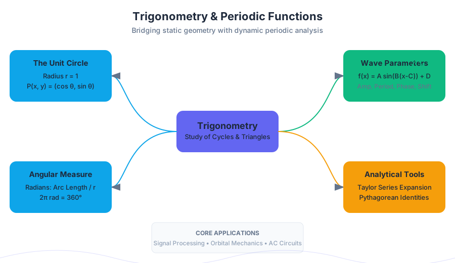
Trigonometry is the mathematical framework that bridges the gap between static geometry and dynamic analysis. While its etymological roots lie in the "measurement of triangles," modern trigonometry is more accurately described as the study of periodic functions—mathematical models that describe cycles, oscillations, and rotations. From the propagation of electromagnetic waves to the orbital mechanics of celestial bodies, trigonometry provides the language for describing any phenomenon that repeats over a fixed interval.

The Unit Circle: The Foundation of Circular Functions

The Unit Circle is a circle with a radius of $r = 1$ centered at the origin $(0,0)$ of the Cartesian coordinate system. It serves as the fundamental reference for defining trigonometric functions beyond the limitations of right-triangle geometry (which is restricted to angles between $0^\circ$ and $90^\circ$).

Defining the Functions

On the unit circle, any angle $\theta$ (measured counter-clockwise from the positive x-axis) determines a point $P(x, y)$. The coordinates of this point are defined as:

Definition: For a point $(x, y)$ on the unit circle at angle $\theta$:

• $\cos(\theta) = x$
• $\sin(\theta) = y$
• $\tan(\theta) = \frac{y}{x} = \frac{\sin(\theta)}{\cos(\theta)}$ (where $x \neq 0$)

This transition from "Opposite/Hypotenuse" to "y-coordinate" allows for the evaluation of trigonometric functions for any real number $\theta$, including negative angles and angles greater than $360^\circ$ ($2\pi$ radians).

Radians vs. Degrees

In advanced mathematics and engineering, radians are the preferred unit of measure. A radian is defined by the arc length of a circle; specifically, one radian is the angle subtended at the center of a circle by an arc equal in length to the radius.

Unit	Full Circle	Right Angle	Conversion Factor
Degrees	$360^\circ$	$90^\circ$	$1^\circ = \frac{\pi}{180}$ rad
Radians	$2\pi$	$\frac{\pi}{2}$	$1 \text{ rad} = \frac{180}{\pi}^\circ$

Common Unit Circle Values

The following table summarizes the exact values for the primary trigonometric functions at standard angles.

$\theta$ (Deg)	$\theta$ (Rad)	$\sin(\theta)$	$\cos(\theta)$	$\tan(\theta)$
$0^\circ$	$0$	$0$	$1$	$0$
$30^\circ$	$\pi/6$	$1/2$	$\sqrt{3}/2$	$\sqrt{3}/3$
$45^\circ$	$\pi/4$	$\sqrt{2}/2$	$\sqrt{2}/2$	$1$
$60^\circ$	$\pi/3$	$\sqrt{3}/2$	$1/2$	$\sqrt{3}$
$90^\circ$	$\pi/2$	$1$	$0$	Undefined
$180^\circ$	$\pi$	$0$	$-1$	$0$
$270^\circ$	$3\pi/2$	$-1$	$0$	Undefined

Low-Level Implementation: Taylor Series Expansion

In computer systems, trigonometric functions are often approximated using CORDIC algorithms or Taylor series expansions when hardware-level instructions are unavailable.

#include <stdio.h>

/**
 * Computes the sine of x using a Taylor Series expansion.
 * sin(x) = x - x^3/3! + x^5/5! - x^7/7! + ...
 * This is a low-level approximation for educational purposes.
 */
double custom_sin(double x) {
    double term = x;
    double sin_x = x;
    int i;
    
    // Normalize x to be within -PI to PI to ensure convergence
    while (x > 3.14159265358979323846) x -= 2 * 3.14159265358979323846;
    while (x < -3.14159265358979323846) x += 2 * 3.14159265358979323846;

    // Perform 10 iterations of the Taylor series
    for (i = 1; i <= 10; i++) {
        term *= -1.0 * x * x / ((2 * i) * (2 * i + 1));
        sin_x += term;
    }
    return sin_x;
}

int main() {
    double angle = 0.523599; // 30 degrees in radians
    printf("sin(30 deg) approx: %f\n", custom_sin(angle));
    return 0;
}

---

Periodic Behavior and Graphing

Trigonometric functions are periodic, meaning they repeat their values in regular intervals. The sine and cosine functions produce "waves" that are essential for modeling everything from sound waves to alternating current (AC).

The General Sine Wave Equation

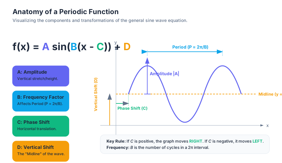
The standard form for a transformed sine or cosine function is: $$f(x) = A \sin(B(x - C)) + D$$

Each parameter controls a specific geometric transformation:

Parameter	Name	Effect	Formula
$\vert A\vert $	Amplitude	Vertical stretch/compression (height of the wave).	$\frac{\text{max} - \text{min}}{2}$
$B$	Frequency Factor	Horizontal stretch/compression.	$B = \frac{2\pi}{P}$
$P$	Period	The distance required for one full cycle.	$P = \frac{2\pi}{\vert B\vert }$
$C$	Phase Shift	Horizontal translation (left/right).	$x = C$
$D$	Vertical Shift	Vertical translation (up/down); the "midline."	$y = D$

Characteristics of Tangent and Reciprocal Functions

Unlike sine and cosine, which are continuous for all real numbers, the tangent, cotangent, secant, and cosecant functions have vertical asymptotes.

• Tangent ($\tan x$): Has a period of $\pi$. Asymptotes occur at $x = \frac{\pi}{2} + n\pi$.
• Secant ($\sec x$): Reciprocal of cosine. It has a range of $(-\infty, -1] \cup [1, \infty)$.

Common Pitfalls in Graphing

1. Period vs. Frequency: Students often confuse $B$ with the period. $B$ is the number of cycles the function completes in a $2\pi$ interval, whereas the period $P$ is the length of a single cycle.
2. Phase Shift Sign: In the expression $(x - C)$, a positive $C$ moves the graph to the right, while a negative $C$ (appearing as $x + |C|$) moves it to the left.
3. Domain Restrictions: When working with inverse trigonometric functions (e.g., $\arcsin(x)$), the domain must be restricted to ensure the inverse is a function.

---

Trigonometric Identities

Identities are equations that are true for all values in the domain of the variable. They are the "algebra" of trigonometry, used to simplify complex expressions and solve equations.

The Pythagorean Identities

Derived directly from the unit circle equation $x^2 + y^2 = 1$:

1. $\sin^2(\theta) + \cos^2(\theta) = 1$
2. $1 + \tan^2(\theta) = \sec^2(\theta)$
3. $1 + \cot^2(\theta) = \csc^2(\theta)$

Sum and Difference Formulas

These are crucial for finding exact values of non-standard angles (e.g., $75^\circ = 45^\circ + 30^\circ$).

• $\sin(\alpha \pm \beta) = \sin \alpha \cos \beta \pm \cos \alpha \sin \beta$
• $\cos(\alpha \pm \beta) = \cos \alpha \cos \beta \mp \sin \alpha \sin \beta$

Double-Angle and Half-Angle Formulas

These allow for the reduction of powers (e.g., changing $\sin^2 x$ into a first-degree cosine expression), which is a vital skill in integral calculus.

Type	Sine	Cosine
Double-Angle	$\sin(2\theta) = 2\sin\theta\cos\theta$	$\cos(2\theta) = \cos^2\theta - \sin^2\theta$
Half-Angle	$\sin(\frac{\theta}{2}) = \pm\sqrt{\frac{1-\cos\theta}{2}}$	$\cos(\frac{\theta}{2}) = \pm\sqrt{\frac{1+\cos\theta}{2}}$

Mathematical Derivation: Law of Cosines

The Law of Cosines is essentially a generalized version of the Pythagorean Theorem that applies to any triangle, not just right triangles.

% Derivation of the Law of Cosines using the Distance Formula
% Consider a triangle with vertices at (0,0), (b,0), and (a cos C, a sin C)

Let the side opposite angle C be 'c'.
The distance formula between (b,0) and (a cos C, a sin C) is:
c^2 = (a cos C - b)^2 + (a sin C - 0)^2

Expanding the terms:
c^2 = a^2 cos^2 C - 2ab cos C + b^2 + a^2 sin^2 C

Rearranging:
c^2 = a^2(cos^2 C + sin^2 C) + b^2 - 2ab cos C

Since cos^2 C + sin^2 C = 1:
c^2 = a^2 + b^2 - 2ab cos C

---

Solving Non-Right Triangles

While basic trigonometry handles right triangles via SOH-CAH-TOA, real-world problems (like navigation or surveying) involve oblique triangles. Two primary laws govern these cases.

1. The Law of Sines

Used when you know a side and its opposite angle. $$\frac{a}{\sin A} = \frac{b}{\sin B} = \frac{c}{\sin C}$$ Best for: AAS (Angle-Angle-Side) or ASA (Angle-Side-Angle) configurations.

The Ambiguous Case (SSA): When given two sides and a non-included angle (Side-Side-Angle), there may be zero, one, or two possible triangles. This occurs because $\sin(\theta) = \sin(180^\circ - \theta)$, meaning an acute angle and an obtuse angle share the same sine value.

2. The Law of Cosines

Used when the Law of Sines cannot be applied. $$c^2 = a^2 + b^2 - 2ab \cos C$$ Best for: SAS (Side-Angle-Side) or SSS (Side-Side-Side) configurations.

Decision Matrix for Solving Triangles

Given Information	Method to Use	Potential Issues
SSS (3 sides)	Law of Cosines	Find the largest angle first to avoid ambiguity.
SAS (2 sides, included angle)	Law of Cosines	No major issues; straightforward.
ASA or AAS	Law of Sines	Very stable; usually one solution.
SSA (2 sides, non-included angle)	Law of Sines	Ambiguous Case: Check for 0, 1, or 2 triangles.

---

Real-World Applications

Trigonometry is the engine behind modern signal processing. Any complex signal—like a human voice or a Wi-Fi data stream—can be decomposed into a sum of simple sine and cosine waves using a Fourier Transform.

Python Example: Signal Summation

This script demonstrates how combining different periodic functions creates a complex wave, a fundamental concept in acoustics and synthesis.

import numpy as np
import matplotlib.pyplot as plt

# Parameters
fs = 1000  # Sampling frequency
t = np.linspace(0, 1, fs)  # 1 second of time

# Generate three different sine waves (Fundamental + Harmonics)
f1, a1 = 5, 1.0    # 5 Hz, Amplitude 1
f2, a2 = 10, 0.5   # 10 Hz, Amplitude 0.5
f3, a3 = 20, 0.2   # 20 Hz, Amplitude 0.2

wave1 = a1 * np.sin(2 * np.pi * f1 * t)
wave2 = a2 * np.sin(2 * np.pi * f2 * t)
wave3 = a3 * np.sin(2 * np.pi * f3 * t)

# Composite wave
complex_wave = wave1 + wave2 + wave3

# Plotting
plt.figure(figsize=(10, 4))
plt.plot(t, complex_wave, label='Summed Signal')
plt.title('Synthesis of a Complex Periodic Signal')
plt.xlabel('Time (s)')
plt.ylabel('Amplitude')
plt.grid(True)
plt.show()

Geospatial Computation: The Haversine Formula

In database systems, calculating the distance between two points on the Earth (a sphere) requires spherical trigonometry. The Haversine formula is a specialized application of the Law of Cosines.

-- SQL implementation of Haversine distance
-- Calculates distance between two points (lat1, lon1) and (lat2, lon2)
SELECT 
    6371 * 2 * ASIN(SQRT(
        POWER(SIN((lat2 - lat1) * PI()/180 / 2), 2) +
        COS(lat1 * PI()/180) * COS(lat2 * PI()/180) *
        POWER(SIN((lon2 - lon1) * PI()/180 / 2), 2)
    )) AS distance_km
FROM locations
WHERE location_id = 101;

---

Advanced Extensions: Euler's Formula

The most profound connection in mathematics involves trigonometry and complex numbers. Euler's Formula states: $$e^{i\theta} = \cos \theta + i \sin \theta$$

This identity shows that circular motion (trigonometry) and exponential growth (calculus) are two sides of the same coin when viewed in the complex plane. It is the basis for Phasor Analysis in electrical engineering, where AC circuits are solved using complex algebra rather than differential equations.

Summary of Key Identities and Properties

Property	Sine ($\sin x$)	Cosine ($\cos x$)	Tangent ($\tan x$)
Parity	Odd ($\sin(-x) = -\sin x$)	Even ($\cos(-x) = \cos x$)	Odd ($\tan(-x) = -\tan x$)
Period	$2\pi$	$2\pi$	$\pi$
Domain	$(-\infty, \infty)$	$(-\infty, \infty)$	$x \neq \frac{\pi}{2} + n\pi$
Range	$[-1, 1]$	$[-1, 1]$	$(-\infty, \infty)$

Analytic Geometry and Intro to Calculus

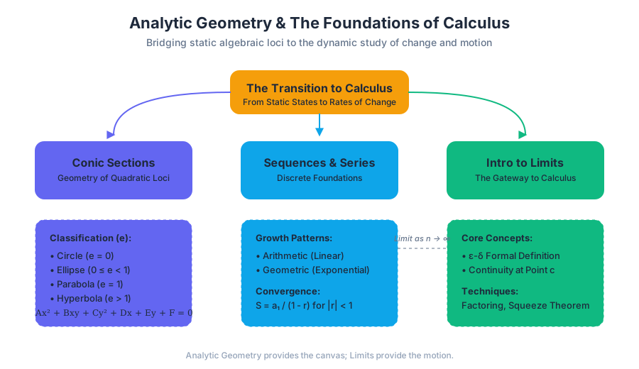
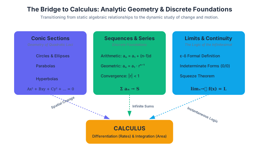
The transition from Precalculus to Calculus represents a fundamental shift in mathematical maturity. While algebra and trigonometry focus on static relationships—solving for $x$ in a fixed state—Calculus introduces the study of change and motion. This section serves as the bridge, formalizing the geometry of curves (Conic Sections), the behavior of discrete patterns (Sequences and Series), and the foundational logic of the infinitesimal (Limits and Continuity).

Conic Sections: The Geometry of Quadratic Loci

Conic sections are the curves obtained by the intersection of a plane with a double-napped right circular cone. Historically, these were studied by Apollonius of Perga, but their modern utility in orbital mechanics, acoustics, and optics stems from their description as algebraic loci.

The General Second-Degree Equation

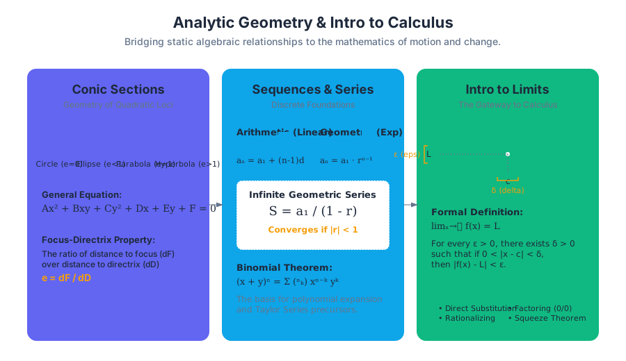
Any conic section can be represented by the general equation: $$Ax^2 + Bxy + Cy^2 + Dx + Ey + F = 0$$ The type of conic is determined by the discriminant $B^2 - 4AC$. In the standard Precalculus curriculum, we often focus on the "non-rotated" case where $B=0$.

Conic Section	Geometric Definition (Locus)	Standard Equation (Center at $h,k$)	Eccentricity ($e$)
Parabola	Points equidistant from a focus and a directrix.	$(x-h)^2 = 4p(y-k)$	$e = 1$
Ellipse	Points where the sum of distances to two foci is constant.	$\frac{(x-h)^2}{a^2} + \frac{(y-k)^2}{b^2} = 1$	$0 \le e < 1$
Hyperbola	Points where the difference of distances to two foci is constant.	$\frac{(x-h)^2}{a^2} - \frac{(y-k)^2}{b^2} = 1$	$e > 1$
Circle	Points at a constant distance from a center.	$(x-h)^2 + (y-k)^2 = r^2$	$e = 0$

Eccentricity and Directrix

The eccentricity ($e$) of a conic section measures how much the conic deviates from being a circle. It is defined as the ratio of the distance from any point on the conic to the focus ($d_F$) and the distance to the directrix ($d_D$): $e = d_F / d_D$.

The Focus-Directrix Property: For any conic section (except the circle), the ratio of the distance from a point $P$ to a fixed point (focus) to the distance from $P$ to a fixed line (directrix) is a constant $e$.

# Low-level implementation: Generating points for an Ellipse
# This script calculates the (x, y) coordinates for an ellipse 
# given its semi-major axis (a) and semi-minor axis (b).

import numpy as np

def generate_ellipse_points(a, b, h=0, k=0, num_points=100):
    """
    Computes points for an ellipse centered at (h, k).
    Formula: x = h + a*cos(t), y = k + b*sin(t)
    """
    t = np.linspace(0, 2 * np.pi, num_points)
    x = h + a * np.cos(t)
    y = k + b * np.sin(t)
    
    # Return as a structured array for engineering use
    return np.column_stack((x, y))

# Example usage for a horizontal ellipse: a=5, b=3
ellipse_data = generate_ellipse_points(5, 3)
print(f"First 5 coordinates:\n{ellipse_data[:5]}")

Sequences and Series: Discrete Foundations

Sequences are ordered lists of numbers, while series represent the sum of those numbers. In the context of Calculus, sequences provide the discrete framework for understanding limits as $n \to \infty$.

Arithmetic vs. Geometric Progressions

1. Arithmetic Sequence: Each term is the previous term plus a constant $d$ (common difference).
   • $n$-th term: $a_n = a_1 + (n-1)d$
   • Sum ($S_n$): $\frac{n}{2}(a_1 + a_n)$
2. Geometric Sequence: Each term is the previous term multiplied by a constant $r$ (common ratio).
   • $n$-th term: $a_n = a_1 \cdot r^{n-1}$
   • Sum ($S_n$): $\frac{a_1(1-r^n)}{1-r}$

Convergence of Infinite Series

An infinite geometric series converges if and only if $|r| < 1$. If it converges, the sum is: $$S = \frac{a_1}{1-r}$$ This concept is the precursor to the Taylor Series in Calculus II, where functions are represented as infinite sums of polynomials.

Feature	Arithmetic	Geometric
Recursive Formula	$a_n = a_{n-1} + d$	$a_n = a_{n-1} \cdot r$
Growth Pattern	Linear	Exponential
Infinite Sum	Always Diverges (unless $a_i=0$)	Converges if $|r| < 1$
Common Application	Simple Interest, Depreciation	Compound Interest, Fractals

\text{The Binomial Theorem expansion for } (x+y)^n:
(x+y)^n = \sum_{k=0}^{n} \binom{n}{k} x^{n-k} y^k
\text{where } \binom{n}{k} = \frac{n!}{k!(n-k)!}

Introduction to Limits: The Gateway to Calculus

The limit is the single most important concept in calculus. It allows us to describe the behavior of a function as the input approaches a value, even if the function is undefined at that specific point.

Formal Definition ($\epsilon-\delta$)

While the intuitive definition is "the value $f(x)$ gets close to," the rigorous definition (the Weierstrass definition) is:

Let $f(x)$ be defined on an open interval containing $c$ (except possibly at $c$). We say $\lim_{x \to c} f(x) = L$ if for every $\epsilon > 0$, there exists a $\delta > 0$ such that if $0 < |x - c| < \delta$, then $|f(x) - L| < \epsilon$.

This definition is essentially a "challenge-response" game: if you tell me how close you want the output to be to $L$ (the $\epsilon$), I can tell you how close $x$ must be to $c$ (the $\delta$).

Limit Laws and Algebraic Manipulation

Evaluating limits often requires bypassing "indeterminate forms" like $0/0$ or $\infty/\infty$.

Technique	When to Use	Example
Direct Substitution	For continuous functions.	$\lim_{x \to 2} x^2 = 4$
Factoring	When substitution yields $0/0$.	$\frac{x^2-4}{x-2} \to \frac{(x-2)(x+2)}{x-2}$
Rationalizing	When square roots create $0/0$.	Multiply by the conjugate.
Squeeze Theorem	When the function is "trapped" between two others.	$\lim_{x \to 0} x^2 \sin(1/x) = 0$

# Real-world usage: Symbolic Math with SymPy (CLI/Python)
# Engineers use symbolic solvers to find limits of complex transfer functions.

python3 -c "
import sympy
x = sympy.Symbol('x')
f = (sympy.sin(x)) / x
result = sympy.limit(f, x, 0)
print(f'The limit of sin(x)/x as x approaches 0 is: {result}')
"

Continuity: The Absence of Breaks

A function is continuous if its graph can be drawn without lifting the pencil. However, in technical terms, continuity at a point requires three distinct conditions to be met.

The Three-Part Definition of Continuity

A function $f(x)$ is continuous at $x = c$ if:

1. $f(c)$ is defined (the point exists).
2. $\lim_{x \to c} f(x)$ exists (the left-hand and right-hand limits match).
3. $\lim_{x \to c} f(x) = f(c)$ (the limit equals the point).

Types of Discontinuity

Understanding where a function fails to be continuous is critical for identifying system instabilities or "shocks" in physical models.

Type	Description	Graphical Representation
Removable	A "hole" in the graph; the limit exists but the point doesn't match.	A line with a single missing dot.
Jump	The left and right limits exist but are not equal.	Common in piecewise/step functions.
Infinite	The function approaches $\pm \infty$ as $x$ approaches $c$.	A vertical asymptote.

The Intermediate Value Theorem (IVT)

The IVT is a powerful existence theorem:

If $f$ is continuous on a closed interval $[a, b]$, and $k$ is any number between $f(a)$ and $f(b)$, then there exists at least one number $c$ in $(a, b)$ such that $f(c) = k$.

Practical Application: The IVT is the mathematical justification for the Bisection Method used in computer science to find roots of equations. If a continuous function changes sign between $a$ and $b$, there must be a zero in between.

// Edge Case: Checking continuity in a piecewise function
// Function: f(x) = { x^2 if x < 2, kx if x >= 2 }
// Find k such that f(x) is continuous at x = 2.

function findContinuityConstant() {
    const c = 2;
    
    // Left-hand limit: x^2 as x -> 2
    const leftLimit = Math.pow(c, 2); 
    
    // Right-hand limit/Value: k * x as x -> 2
    // We need: k * 2 = leftLimit
    const k = leftLimit / c;
    
    console.log(`For the function to be continuous, k must be: ${k}`);
    return k;
}

findContinuityConstant(); // Output: 2

Synthesis: Connecting the Dots

The concepts in this section are not isolated. They represent a progression of complexity:

1. Conics define the paths of objects (like a planet's orbit).
2. Sequences allow us to sample that path at discrete intervals.
3. Limits allow us to shrink those intervals to zero.
4. Continuity ensures that the path is a smooth, predictable trajectory rather than a series of disjointed teleports.

In Calculus I, you will use the limit to define the Derivative (the slope of a tangent line to a conic) and the Integral (the area under a curve). Without the rigorous definitions of limits and continuity established here, the entire edifice of modern physics and engineering would lack a logical foundation.

Common Pitfalls and Misconceptions

• Limit vs. Value: A common mistake is assuming $\lim_{x \to c} f(x)$ must equal $f(c)$. The limit describes the neighborhood, while $f(c)$ describes the point. They only agree if the function is continuous.
• Divergence of Harmonic Series: Students often assume that if the terms of a series go to zero ($a_n \to 0$), the series must converge. The Harmonic Series ($\sum 1/n$) is the classic counterexample: the terms get smaller, but the sum grows to infinity.
• Hyperbola Asymptotes: Unlike a parabola, which opens wider and wider, a hyperbola is constrained by linear asymptotes $y = \pm \frac{b}{a}(x-h) + k$. Confusing the two leads to significant errors in trajectory modeling.
• The "0/0" Trap: $0/0$ is not 1, and it is not 0. It is indeterminate, meaning more work (factoring, rationalizing) is required to find the actual limit.