pandas documentation
Institution: MIT
38 study materials · 7 sections
This DeepWiki provides a comprehensive guide to the pandas library, version 3.0.2, based on its official documentation. It is designed to take learners from installation and foundational concepts, such as the DataFrame and Series data structures, through hands-on tutorials on data wrangling, manipulation, and visualization. The course also includes advanced topics like time series analysis, guides for users transitioning from other tools like SQL and R, and resources for developers looking to master the API or contribute to the project.
Course Sections
Introduction to pandas
Key concepts: Installation (conda/pip) · Virtual Environments · Primary Data Structures (Series & DataFrame) · Core Features for Data Manipulation · Data Representation
This section introduces the pandas library, covering its purpose, core data structures (DataFrame and Series), and installation. It provides the foundational knowledge needed to understand why and how pandas is used for data analysis in Python.
Introduction to pandas
Pandas is an open-source Python library that has become the de facto standard for data manipulation and analysis in the scientific Python ecosystem. Its name is derived from "panel data," an econometrics term for multidimensional structured data sets. Built on top of the NumPy library, pandas provides high-performance, easy-to-use data structures and data analysis tools designed to make working with labeled and relational data both intuitive and efficient. It excels at handling tabular data, heterogeneous columns, and time-series data, bridging the gap between raw data and sophisticated analysis or machine learning models.
At its core, pandas solves a fundamental problem: how to represent and interact with structured data within Python in a way that is both computationally efficient and semantically expressive. Before pandas, data analysts often juggled lists of lists, dictionaries of dictionaries, or NumPy arrays, all of which had significant limitations for the common tasks of cleaning, transforming, filtering, and aggregating real-world datasets. Pandas introduces two primary data structures, the DataFrame and the Series, which provide an integrated, index-aware framework for these tasks, fundamentally changing the landscape of data science in Python.
AI_SVGI_SVG## Installation and Environment Management
Before diving into the library's features, a robust and isolated development environment is paramount. This prevents conflicts between project dependencies and ensures reproducibility. The two most common package managers in the Python data ecosystem are conda and pip.
What it is
Installation is the process of adding the pandas library and its dependencies to your Python environment. A virtual environment is an isolated directory tree that contains a specific Python installation and any additional packages. Working within a virtual environment is a critical best practice.
Why it matters
Data science projects often rely on a complex web of libraries (e.g., pandas, numpy, scikit-learn, matplotlib, tensorflow), each with its own version requirements. Installing everything into the global Python installation can lead to a "dependency hell," where upgrading one package breaks another. Virtual environments solve this by creating a self-contained sandbox for each project. This ensures that your project's dependencies are explicit, consistent across different machines, and do not interfere with other projects.
How it works
Both conda and pip manage package installation, but they operate at different levels. pip is the standard package installer for Python and manages Python packages only. conda is a cross-platform, language-agnostic package and environment manager. It can manage Python packages but also Python itself, as well as non-Python libraries (e.g., C/C++ libraries like MKL or CUDA) that are often dependencies for high-performance scientific packages.
| Feature | conda (via Anaconda/Miniconda) |
pip (with venv) |
|---|---|---|
| Scope | Language-agnostic (Python, R, C++, etc.) | Python-specific |
| Environment Mgmt | Built-in (conda create, conda activate) |
Separate module (venv) |
| Package Source | Anaconda repositories (curated, pre-compiled) | Python Package Index (PyPI) |
| Dependency Resolution | Advanced solver, checks for compatibility across all packages (Python and non-Python) | Can be less robust, especially with complex binary dependencies; newer versions have improved. |
| Typical Use Case | Scientific computing, data science, ML (where binary dependencies are common) | General Python development, web development |
Concrete Example: Setting up an Environment
Here is a typical workflow for creating and activating a virtual environment and installing pandas using conda. This is the recommended approach for most data science applications.
# 1. Create a new conda environment named 'data-analysis' with Python 3.11
#    Conda will resolve and install Python and other base packages.
conda create --name data-analysis python=3.11

# 2. Activate the newly created environment.
#    Your shell prompt will change to indicate you are in the environment.
conda activate data-analysis

# 3. Install pandas, numpy, and matplotlib from the conda-forge channel.
#    conda-forge is a community-led channel with a vast collection of packages.
#    Specifying versions ensures reproducibility.
conda install -c conda-forge pandas==2.2.1 numpy==1.26.4 matplotlib==3.8.3

# 4. Verify the installation by checking the pandas version.
python -c "import pandas as pd; print(pd.__version__)"

# 5. When finished, deactivate the environment to return to the base shell.
conda deactivate
This sequence of commands provides a clean, reproducible, and high-performance environment for any data analysis project. Using a requirements file (environment.yml for conda or requirements.txt for pip) is the next step for professional project management.
Primary Data Structures: Series and DataFrame
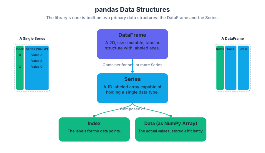
Pandas represents data in two fundamental structures: the Series and the DataFrame. Mastering these two objects is the key to unlocking the full power of the library. They are not merely containers for data; they are sophisticated objects with a rich API for transformation and analysis.
The Series
A Series is a one-dimensional, array-like object containing a sequence of values of a single data type, and an associated array of data labels, called its index.
What it is
Think of a Series as a smart, labeled array. It is composed of two primary components:
- Data: A sequence of values, typically a NumPy
ndarrayunder the hood. This allows for highly efficient, vectorized operations. - Index: An object (of type
pd.Index) that provides labels for the data. These labels can be integers, strings, dates, or other hashable types. The index allows for fast lookups and alignment of data.
A Series can also have a name attribute, which is useful for identifying it, especially when it's a column in a DataFrame.
How it works
Let's demystify the Series by building a simplified version from scratch. This illustrates the core concept of coupling a data array with an index for labeled access.
import numpy as np

class SimpleSeries:
    """A simplified implementation of a pandas-like Series."""
    def __init__(self, data, index=None, name=None):
        if not isinstance(data, (list, np.ndarray)):
            raise TypeError("Data must be a list or NumPy array.")

        self._data = np.asarray(data)
        self.name = name

        if index is None:
            # Default to a range index if none is provided
            self._index = np.arange(len(self._data))
        else:
            if len(data) != len(index):
                raise ValueError("Length of data and index must be the same.")
            self._index = np.asarray(index)

        # Create a mapping from index label to integer position for fast lookups
        self._index_map = {label: pos for pos, label in enumerate(self._index)}

    def __len__(self):
        return len(self._data)

    def __repr__(self):
        output = ""
        for i, val in zip(self._index, self._data):
            output += f"{str(i):<10} {str(val)}\n"
        dtype_str = f"dtype: {self._data.dtype}"
        name_str = f"Name: {self.name}, " if self.name else ""
        return f"{output}\n{name_str}Length: {len(self)}, {dtype_str}"

    def __getitem__(self, key):
        # Support both positional and label-based access
        if isinstance(key, int):
            return self._data[key]
        elif key in self._index_map:
            pos = self._index_map[key]
            return self._data[pos]
        else:
            raise KeyError(f"Label not found in index: {key}")

    @property
    def values(self):
        return self._data

    @property
    def index(self):
        return self._index

# Example Usage
population_data = SimpleSeries(
    [38_250_000, 39_510_000, 29_140_000],
    index=['Canada', 'California', 'Texas'],
    name='Population'
)
print(population_data)
print(f"\nPopulation of California: {population_data['California']}")
This simple class captures the essence of a pandas Series: it binds data (_data) to an index (_index) and provides a lookup mechanism (__getitem__) that can work with labels. The real pandas Series is, of course, vastly more complex, with hundreds of optimized methods, robust data type handling, and seamless integration with the rest of the library.
The DataFrame
A DataFrame is a two-dimensional, size-mutable, and potentially heterogeneous tabular data structure with labeled axes (rows and columns).
What it is
A DataFrame is the primary workhorse of pandas. It is best conceptualized in several ways:
- As a spreadsheet or SQL table in memory.
- As a dictionary of Series objects, where the keys are the column names and the values are the Series themselves, all sharing a common index.
It has both a row index and a column index, making it a powerful tool for selecting, aligning, and manipulating data. Each column can have a different data type (e.g., numbers, strings, dates, booleans), which makes it heterogeneous.
Concrete Example: Creating and Inspecting a DataFrame
Let's create a DataFrame from scratch and use some fundamental inspection methods. We'll use the Titanic dataset for this and subsequent examples.
import pandas as pd
import numpy as np

# Load data from a URL
# Using specific dtypes during read can save memory and prevent errors
titanic_df = pd.read_csv(
    "https://raw.githubusercontent.com/pandas-dev/pandas/main/doc/data/titanic.csv",
    usecols=['Survived', 'Pclass', 'Name', 'Sex', 'Age', 'Fare'],
    dtype={'Pclass': 'category', 'Survived': 'int8'}
)

# Inspect the first few rows
print("--- First 5 rows (head) ---")
print(titanic_df.head())

# Get a concise summary of the DataFrame
# This is invaluable for initial data exploration
print("\n--- Technical Summary (info) ---")
titanic_df.info()

# Generate descriptive statistics for numerical columns
print("\n--- Descriptive Statistics (describe) ---")
print(titanic_df.describe())
The output of .info() is particularly revealing. It shows the row index type and count (RangeIndex: 891 entries), the total number of columns, and for each column: its name, the count of non-null values, and its data type (Dtype). This single command provides a comprehensive overview of the DataFrame's structure and potential data quality issues (like missing values in the Age column).
Series vs. DataFrame
| Aspect | pd.Series |
pd.DataFrame |
|---|---|---|
| Dimensions | 1-D | 2-D |
| Data Structure | Homogeneous labeled array | Heterogeneous labeled table |
| Analogy | A single column in a spreadsheet | An entire spreadsheet or SQL table |
| Components | Data, Index, Name, Dtype | Data, Index (rows), Columns |
| Creation | pd.Series(data, index=...) |
pd.DataFrame(data, index=..., columns=...) |
| Relationship | A column of a DataFrame is a Series. | A collection of Series sharing a common index. |
Core Features for Data Manipulation
A DataFrame is not just a static data container; it is an object with a rich set of methods for transformation and analysis. The power of pandas lies in its ability to perform these operations efficiently and expressively.
Data Ingestion and Representation
Pandas provides a suite of read_* functions for ingesting data from various formats, with pd.read_csv being the most common. These functions are highly optimized and offer dozens of parameters to handle real-world messy data.
Once loaded, the data is represented in memory using a block-based architecture. Columns of the same data type are often grouped together in NumPy arrays, a structure known as the BlockManager. This internal architecture is key to pandas' performance, as it allows NumPy's fast, vectorized C-level operations to be applied to entire blocks of data at once.
Key Insight: Pandas operations are vectorized. This means that operations are applied to entire arrays (Series or columns) at once, rather than iterating over elements one by one in Python. This delegation to underlying, compiled C or Cython code is the primary source of pandas' speed. Avoid writing explicit
forloops over DataFrame rows whenever possible.
Selection and Subsetting (.loc, .iloc)
One of the most common tasks is selecting subsets of data. Pandas provides a powerful and precise syntax for this, which can be a point of confusion for beginners.
| Method | Selection By | Input Type | Behavior | Common Use Case |
|---|---|---|---|---|
df[...] |
Column(s) or Rows | String, list of strings, or boolean array | Ambiguous: selects columns by name, but can slice rows with df[0:5] or filter rows with a boolean mask. |
Quick, interactive column selection (df['Age']) or boolean filtering (df[df['Age'] > 30]). |
df.loc[...] |
Labels | Row labels, column labels | Explicitly label-based. Slices are inclusive of the endpoint. | Selecting data by meaningful index labels (e.g., dates, names) or boolean conditions. |
df.iloc[...] |
Integer Position | Row integers, column integers | Explicitly position-based. Slices are exclusive of the endpoint, like standard Python. | Selecting data by its numerical position, regardless of index labels. |
Common Pitfall: Chained Indexing
A frequent mistake is using chained indexing for assignment, like df[df['Age'] > 60]['Survived'] = 0. This can lead to a SettingWithCopyWarning and unpredictable results because the first indexing operation (df[df['Age'] > 60]) might return a copy of the data, not a view. The subsequent assignment then modifies this temporary copy, which is immediately discarded, leaving the original DataFrame unchanged.
The correct, idiomatic way to perform this assignment is with a single .loc call:
# Create a copy to avoid modifying the original df in later examples
titanic_subset = titanic_df.copy()

# --- INCORRECT: Chained assignment ---
# This may or may not work and raises a warning.
# titanic_subset[titanic_subset['Age'] > 65]['Fare'] = 0

# --- CORRECT: Using .loc for assignment ---
# Select rows based on a boolean condition and columns by label, then assign.
titanic_subset.loc[titanic_subset['Age'] > 65, 'Fare'] = 0
print("Fare for passengers over 65 set to 0:")
print(titanic_subset[titanic_subset['Age'] > 65].head())
The Split-Apply-Combine Strategy
Many complex data analysis problems can be framed using the split-apply-combine paradigm, a concept popularized by Hadley Wickham. Pandas' groupby() operation is the canonical implementation of this pattern.
- Split: The data is split into groups based on some criteria (e.g., by
SexandPclass). - Apply: A function is applied independently to each group (e.g., calculate the mean
Ageor the survival rate). - Combine: The results of the function applications are combined into a new data structure.
Concrete Example: Groupby Aggregation
Let's calculate the average age and survival rate for passengers, grouped by their class and sex.
# Group by passenger class and sex
grouped = titanic_df.groupby(['Pclass', 'Sex'])

# Apply multiple aggregation functions at once using a dictionary
# This is highly efficient and expressive.
agg_results = grouped.agg(
    mean_age=('Age', 'mean'),
    median_fare=('Fare', 'median'),
    survival_rate=('Survived', 'mean'),
    count=('Survived', 'count')
)

# The result is a DataFrame with a MultiIndex
print(agg_results.round(2))
This single, expressive command replaces what would be a complex series of loops and conditional logic in traditional programming. It clearly demonstrates the power of the split-apply-combine pattern for summarizing data.
This introduction has covered the foundational concepts of pandas: its purpose, proper setup, the core Series and DataFrame structures, and an overview of its main features. With this foundation, you are equipped to explore the vast capabilities of the library for cleaning, transforming, modeling, and visualizing data.
Core Data Wrangling: A Hands-On Guide
Key concepts: Data I/O (read_csv, to_excel) · Subsetting & Filtering (loc, iloc) · Column Creation & Renaming · Grouping & Aggregation (groupby) · Combining & Merging Data (concat, merge) · Reshaping Data (pivot, melt) · Data Visualization (plot)
A practical, hands-on guide covering the most essential data manipulation tasks. This section walks through reading/writing data, selecting subsets, creating new columns, calculating statistics, reshaping tables, and combining data from multiple sources.
Core Data Wrangling: A Hands-On Guide
Data wrangling, often called data munging, is the foundational process of transforming and mapping raw data from one form into another with the intent of making it more appropriate and valuable for a variety of downstream purposes such as analytics. It is an iterative process that encompasses the cleaning, structuring, and enriching of data. In practice, data scientists and analysts report that this phase consumes up to 80% of their time. Mastering these core operations is not merely a technical skill; it is the art and science of preparing a clean canvas for analytical inquiry. This guide provides a hands-on, technically precise tour of the essential data wrangling operations using the pandas library, the de facto standard for data manipulation in Python.
AI_SVGI_SVG## Data I/O: The Gateway to Analysis
What It Is
Data Input/Output (I/O) is the process of loading data from an external source (like a file, database, or API) into an in-memory data structure, and conversely, saving the processed data from memory back to a persistent storage medium. In pandas, this typically means reading data into a DataFrame and writing a DataFrame out to a file.
Why It Matters
Data rarely originates within your analysis script. It resides in comma-separated value (CSV) files, Excel spreadsheets, SQL databases, or web APIs. Effective I/O is the crucial first step that brings this external data into your analytical environment and the final step that shares your results. The robustness and efficiency of your I/O operations can significantly impact the performance and reliability of your entire data pipeline, especially with large datasets.
How It Works: Reading and Writing Files
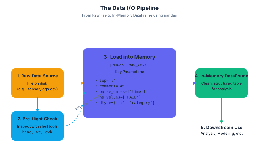
The most common data format for tabular data is CSV. The pandas function pd.read_csv() is a highly optimized and flexible tool for parsing these files. It goes far beyond simply splitting lines by commas; it involves type inference (detecting integers, floats, dates), handling headers, managing missing values, and dealing with various text encodings.
Conversely, df.to_excel() serializes a DataFrame into an Excel workbook (.xlsx format). This process leverages underlying libraries (like openpyxl or xlsxwriter) to construct the file format, writing data cells, headers, and the index, and can even handle writing to multiple sheets within the same workbook.
Let's examine a practical, non-trivial example of reading a dataset of sensor logs. These logs might have a non-standard delimiter, comments to ignore, and specific columns that should be parsed as dates.
# Python: Advanced pd.read_csv() usage
import pandas as pd
from io import StringIO

# Simulate a complex CSV file content
# Note the semicolon delimiter, commented header, and specific date/time format
csv_data = """# Sensor Log Data
# Collected on: 2023-10-27
sensor_id;timestamp;reading_1;reading_2;status
A-01;27/10/2023 08:00:15;10.5;88.1;OK
B-02;27/10/2023 08:00:18;22.1;15.4;FAIL
A-01;27/10/2023 08:01:20;10.6;88.3;OK
C-03;27/10/2023 08:01:22;;45.9;OK
"""

# Use StringIO to simulate reading from a file
data_file = StringIO(csv_data)

# Read the data using advanced parameters
df = pd.read_csv(
    data_file,
    sep=';',                     # Specify the semicolon delimiter
    comment='#',                 # Ignore lines starting with '#'
    header=0,                    # The first non-commented line is the header
    names=['id', 'time', 'r1', 'r2', 'result'], # Provide new column names
    parse_dates=['time'],        # Parse the 'time' column as datetime objects
    dayfirst=True,               # Ambiguous date format (DD/MM/YYYY)
    na_values=['', 'FAIL'],     # Treat empty strings and 'FAIL' as missing data (NaN)
    dtype={'id': 'category'}     # Optimize memory for the 'id' column
)

print(df.info())
print(df)
Before even attempting to load a large, unfamiliar file in Python, a prudent first step is to inspect it using command-line tools. This avoids memory errors and provides crucial metadata for crafting the correct read_csv call.
# Shell: Inspecting a CSV file before loading
# Assume the data is in a file named 'sensor_logs.csv'

# 1. View the first 5 lines to check the header and delimiter
$ head -n 5 sensor_logs.csv
# Sensor Log Data
# Collected on: 2023-10-27
# sensor_id;timestamp;reading_1;reading_2;status
# A-01;27/10/2023 08:00:15;10.5;88.1;OK
# B-02;27/10/2023 08:00:18;22.1;15.4;FAIL

# 2. Count the total number of lines to gauge file size
$ wc -l sensor_logs.csv
# 6 sensor_logs.csv

# 3. Use awk to check the number of fields in each line (using ';' as delimiter)
# This helps identify malformed rows. NF is the Number of Fields.
$ awk -F';' '{print NF}' sensor_logs.csv
# 1
# 1
# 5
# 5
# 5
# 5
This shell-level inspection reveals the semicolon delimiter, the two comment lines, and the consistent 5-column structure, informing the parameters we used in the Python code.
pd.read_csv Parameter |
Purpose | Common Use Case |
|---|---|---|
filepath_or_buffer |
The path to the file or a file-like object. | '/path/to/data.csv' or a URL. |
sep or delimiter |
The character sequence separating values. | ',' (default), '\t' for tab-separated, ';'. |
header |
Row number to use as column names. | 0 (default), None if no header. |
names |
A list of column names to use. | Used when header=None or to override existing headers. |
index_col |
Column to use as the row labels (index). | 0 to use the first column. |
dtype |
A dictionary mapping column names to data types. | {'user_id': str, 'value': float} to prevent incorrect type inference. |
parse_dates |
List of columns to parse as dates. | ['timestamp', 'event_date']. |
na_values |
Additional strings to recognize as NaN. |
['Not Available', 'N/A', -1]. |
chunksize |
An integer for iterating over a large file in chunks. | 100000 to process a multi-gigabyte file without loading it all into memory. |
Common Pitfalls
- Encoding Errors: Files saved with non-standard encoding (e.g.,
latin1) will raise aUnicodeDecodeErrorif not read with the correctencodingparameter. Always default toencoding='utf-8'if unsure. - Mixed Data Types: A column containing both numbers and text will be inferred as type
object, which is inefficient. This often triggers aDtypeWarning. Use thedtypeparameter to specify types explicitly or investigate the source of the mixed types. - Memory Overload: Attempting to load a file larger than available RAM will crash the session. For large files, use the
chunksizeparameter inread_csvto process the file piece by piece, or consider more scalable tools like Dask or Polars.
Subsetting & Filtering: The Art of Selection
What It Is
Subsetting is the process of extracting a portion of your data. This can involve selecting specific columns (projection), specific rows (selection), or a combination of both. Filtering is a form of subsetting rows based on one or more logical conditions. pandas provides a rich set of accessors for this purpose, primarily .loc, .iloc, and boolean indexing.
Definition: Accessors In
pandas, accessors like.locand.ilocare properties that provide a dedicated namespace for a specific type of indexing. They are not methods (called with()), but are used with square brackets[]. This design avoids ambiguity in the standard[]operator.
Why It Matters
Raw datasets are often vast and contain information irrelevant to the specific question at hand. Effective subsetting is the primary way to isolate the signal from the noise, focusing your computational resources and analytical attention on the relevant data. It is the pandas equivalent of the WHERE clause in SQL or filtering in a spreadsheet.
How It Works: Label vs. Position
pandas makes a critical distinction between label-based and position-based indexing.
.loc(Label-based): Selects data based on the index labels and column names. The slicing is inclusive of the endpoint.df.loc['start_label':'end_label']includes'end_label'..iloc(Integer-position-based): Selects data based on its integer position (from0tolength-1). The slicing follows Python's convention and is exclusive of the endpoint.df.iloc[0:5]includes positions 0, 1, 2, 3, and 4.- Boolean Indexing: A
SeriesofTrue/Falsevalues, with the same index as theDataFrame, can be passed to.locor the[]operator to select only the rows where the value isTrue.
Consider a dataset of employee records. We want to find all senior engineers in the R&D department hired after 2020. This requires a combination of column selection and conditional row filtering.
# Python: Complex filtering with .loc and boolean indexing
import pandas as pd
import numpy as np

# Create a sample DataFrame
data = {
    'employee_id': range(101, 111),
    'name': [f'Emp_{i}' for i in range(10)],
    'department': ['R&D', 'Sales', 'R&D', 'HR', 'R&D', 'Sales', 'R&D', 'HR', 'Sales', 'R&D'],
    'title': ['Engineer', 'Manager', 'Senior Engineer', 'Recruiter', 'Engineer', 'Analyst', 'Senior Engineer', 'Manager', 'Analyst', 'Data Scientist'],
    'hire_date': pd.to_datetime(['2019-03-15', '2018-07-22', '2021-01-10', '2022-05-30', '2023-08-01', '2019-11-12', '2022-02-14', '2021-09-01', '2023-04-18', '2020-12-01']),
    'salary': [75000, 110000, 120000, 65000, 82000, 70000, 135000, 105000, 72000, 150000]
}
employees = pd.DataFrame(data).set_index('employee_id')

# Define the conditions for filtering
is_rd = employees['department'] == 'R&D'
is_senior_engineer = employees['title'] == 'Senior Engineer'
hired_after_2020 = employees['hire_date'] > '2020-12-31'

# Combine conditions and apply the filter using .loc
# Select only the 'name', 'title', and 'salary' columns for the filtered rows
result = employees.loc[
    (is_rd & is_senior_engineer) & hired_after_2020,
    ['name', 'title', 'salary']
]

print(result)
This same logical query can be expressed elegantly in SQL, highlighting the conceptual parallels between database querying and DataFrame manipulation.
-- SQL: Equivalent filtering query
SELECT
    name,
    title,
    salary
FROM
    employees
WHERE
    department = 'R&D'
    AND title = 'Senior Engineer'
    AND hire_date > '2020-12-31';
| Feature | .loc |
.iloc |
|---|---|---|
| Selection By | Label | Integer Position |
| Arguments | Index/column labels | Integers, slices of integers |
| Slicing Endpoint | Inclusive (df.loc['a':'c'] includes 'c') |
Exclusive (df.iloc[0:3] includes 0, 1, 2) |
| Error Handling | KeyError if a label is not found |
IndexError if an integer is out of bounds |
| Use Case | When index/column names are meaningful and stable | When you need positional access, regardless of labels |
Common Pitfalls
- Chained Indexing and
SettingWithCopyWarning: A very common mistake is to use two sets of brackets to select and assign, likedf[df['col1'] > 0]['col2'] = 100. This is called chained indexing.pandascannot guarantee whether the first operation returns a view or a copy of the data, so the assignment might fail silently. This raises aSettingWithCopyWarning. - The Correct Approach: Always use
.locfor simultaneous row and column selection when assigning:df.loc[df['col1'] > 0, 'col2'] = 100. This is a single, unambiguous operation that always modifies the originalDataFrame.
Column Creation & Renaming: Shaping the Schema
What It Is
This involves two related operations:
- Column Creation: Adding new columns to a
DataFrame, typically derived from calculations on existing columns. This is the primary mechanism for feature engineering. - Column Renaming: Modifying the labels of columns (or the index) to be more descriptive, to conform to a standard, or to remove problematic characters.
Why It Matters
Raw data often lacks the explicit features needed for modeling or analysis. For example, a dataset might contain birth_date but not age, or revenue and cost but not profit. Creating these derived columns is a fundamental step in enriching the dataset. Renaming columns is a matter of good housekeeping, making the data easier to understand and work with, especially for collaborators.
How It Works: Vectorization and Chaining
The most efficient way to create new columns is through vectorized operations. Instead of looping through rows, you apply operations to entire Series at once. pandas, built on NumPy, is highly optimized for this.
There are two main syntactic styles for this:
- Direct Assignment: The classic
df['new_column'] = ...syntax. It's simple and modifies theDataFramein place. .assign()Method: A functional approach,df.assign(new_column=...). It does not modify the originalDataFramebut returns a new one with the added column. This makes it ideal for method chaining.
For renaming, the .rename() method is the standard tool. It accepts a dictionary mapping old names to new names.
# Python: Column creation and renaming
import pandas as pd
import numpy as np

# Sample sales data
sales_data = {
    'order_id': ['O1', 'O2', 'O3', 'O4'],
    'product_name': ['Widget A', 'Widget B', 'Widget A', 'Widget C'],
    'unit_price_usd': [10.00, 25.50, 10.25, 5.75],
    'quantity': [5, 2, 10, 8]
}
sales = pd.DataFrame(sales_data)

# --- Column Creation ---
# 1. Direct assignment (vectorized operation)
sales['total_price_usd'] = sales['unit_price_usd'] * sales['quantity']

# 2. Using .assign() for chaining, and a more complex function
# Let's add a 5% tax and convert to EUR (assume 1 USD = 0.92 EUR)
exchange_rate = 0.92
final_sales = (
    sales
    .assign(
        total_price_eur=lambda df: df['total_price_usd'] * 1.05 * exchange_rate,
        category=lambda df: df['product_name'].str.split().str[0]
    )
    # --- Renaming ---
    # Rename columns to a more standard format
    .rename(columns={
        'unit_price_usd': 'unit_price',
        'total_price_eur': 'final_price_eur',
        'quantity': 'units_sold'
    })
)

print("Original DataFrame:")
print(sales)
print("\nTransformed DataFrame:")
print(final_sales)
The same transformations can be achieved in R using the popular dplyr library, which heavily emphasizes a chainable, "pipe-based" workflow that is conceptually similar to pandas's method chaining.
# R/dplyr: Equivalent data manipulation
library(dplyr)

# Create the initial data frame
sales_data <- data.frame(
  order_id = c('O1', 'O2', 'O3', 'O4'),
  product_name = c('Widget A', 'Widget B', 'Widget A', 'Widget C'),
  unit_price_usd = c(10.00, 25.50, 10.25, 5.75),
  quantity = c(5, 2, 10, 8)
)

exchange_rate <- 0.92

# Use pipes (%>%) to chain operations
final_sales <- sales_data %>%
  # Create new columns with mutate()
  mutate(
    total_price_usd = unit_price_usd * quantity,
    final_price_eur = total_price_usd * 1.05 * exchange_rate,
    category = sapply(strsplit(product_name, " "), `[`, 1)
  ) %>%
  # Rename columns with rename()
  rename(
    unit_price = unit_price_usd,
    units_sold = quantity
  )

print(final_sales)
Grouping & Aggregation: Summarizing with Precision
What It Is
Grouping and Aggregation is a powerful process for computing summary statistics on subsets of data. It is famously described by the "split-apply-combine" paradigm:
- Split: The data is partitioned into groups based on the values in one or more key columns.
- Apply: A function (the aggregation) is applied independently to each group. This could be a sum, mean, count, or a custom function.
- Combine: The results of the function applications are combined into a new
DataFrame.
The cornerstone of this process in pandas is the .groupby() method.
AI_DEMOI_DEMO### Why It Matters Raw, row-level data is often too granular to reveal meaningful patterns. Aggregation allows you to zoom out and see the bigger picture. How do sales compare across different regions? What is the average patient recovery time for different treatment groups? What is the maximum error rate per sensor type? These are all questions that can only be answered through grouping and aggregation. It is the engine of descriptive analytics.
How It Works: The GroupBy Object
Calling df.groupby('key_column') does not immediately compute anything. Instead, it returns a DataFrameGroupBy object. This is a lazy object that holds all the information needed to perform computations on the groups. The actual calculation happens only when an aggregation method (like .sum(), .mean(), .size(), or .agg()) is called on this object.
The .agg() method is the most flexible, allowing you to apply multiple functions at once, and even apply different functions to different columns.
# Python: Advanced aggregation with .groupby().agg()
import pandas as pd

# Sample dataset of customer transactions
data = {
    'customer_id': ['C1', 'C2', 'C1', 'C3', 'C2', 'C1'],
    'region': ['North', 'South', 'North', 'North', 'West', 'West'],
    'product_category': ['Electronics', 'Apparel', 'Home Goods', 'Electronics', 'Apparel', 'Electronics'],
    'sales': [1200, 150, 450, 800, 200, 1500],
    'quantity': [1, 3, 2, 1, 4, 2]
}
transactions = pd.DataFrame(data)

# Group by region and customer, then compute multiple aggregations
# We want total sales, average sale amount, and number of unique product categories per group
summary = transactions.groupby(['region', 'customer_id']).agg(
    total_sales=('sales', 'sum'),
    average_sale=('sales', 'mean'),
    distinct_categories=('product_category', 'nunique'),
    number_of_transactions=('sales', 'count')
)

print(summary)
This split-apply-combine pattern is a direct analogue to SQL's GROUP BY clause, which is the canonical implementation of this idea in the database world.
-- SQL: Equivalent GROUP BY query
SELECT
    region,
    customer_id,
    SUM(sales) AS total_sales,
    AVG(sales) AS average_sale,
    COUNT(DISTINCT product_category) AS distinct_categories,
    COUNT(sales) AS number_of_transactions
FROM
    transactions
GROUP BY
    region,
    customer_id
ORDER BY
    region,
    customer_id;
Variations: transform and filter
While agg returns a reduced summary, groupby has other powerful methods:
.transform(func): Applies a function to each group but returns aSeriesorDataFramewith the same index as the original. This is useful for creating group-level features, like a column showing the average sales for each customer's region on every transaction row..filter(func): Takes a function that returnsTrueorFalsefor each group. It then returns a subset of the originalDataFramecontaining only the rows from groups where the function returnedTrue. This is useful for discarding groups that don't meet a certain criterion (e.g., keeping only customers with more than 2 transactions).
GroupBy Method |
Output Shape | Common Use Case |
|---|---|---|
agg() |
Reduced; one row per group. | Calculating summary statistics (sum, mean, count). |
transform() |
Same as input. | Creating new columns based on group properties (e.g., z-scores within a group). |
filter() |
Subset of input rows. | Dropping entire groups based on a condition (e.g., groups with too few members). |
Combining & Merging Data: Assembling the Puzzle
What It Is
Combining is the process of integrating data from two or more DataFrames into a single one. pandas provides two primary mechanisms for this:
pd.concat(): StacksDataFrameson top of each other (row-wise,axis=0) or side-by-side (column-wise,axis=1). It aligns data based on the index.pd.merge(): Performs database-style joins onDataFrames. It combines them based on the values in one or more common columns (the "keys").
Why It Matters
In any real-world project, data is fragmented. Customer information might be in one table, their orders in another, and product details in a third. To get a complete picture—for instance, to find the total sales for customers in a specific demographic—you must combine these disparate datasets. Merging is the core operation for linking related data.
How It Works: Concatenation vs. Merging
Concatenation is like gluing pieces of paper together. It's a simple, positional operation. When concatenating by rows, pandas appends the rows and aligns the columns. If a column exists in one DataFrame but not another, it will be filled with NaN in the respective rows.
Merging, on the other hand, is a more sophisticated, value-based operation rooted in relational algebra. It combines rows from two DataFrames where the values in their key columns match. The type of join determines how to handle keys that don't exist in both DataFrames.
Definition: Join Types
- Inner Join: Returns only the rows where the key exists in both
DataFrames. This is the intersection of the keys.- Left Join: Returns all rows from the left
DataFrame, and the matched rows from the rightDataFrame. If there is no match for a key from the leftDataFrame, the columns from the right will beNaN.- Right Join: The reverse of a left join. Returns all rows from the right
DataFrame.- Outer Join: Returns all rows when there is a match in either the left or the right
DataFrame. This is the union of the keys.
Let's say we have one DataFrame with employee details and another with their department information. We can use a merge to add the department name and location to each employee's record.
# Python: A realistic pd.merge() example
import pandas as pd

employees = pd.DataFrame({
    'emp_id': ['E1', 'E2', 'E3', 'E4', 'E5'],
    'name': ['Alice', 'Bob', 'Charlie', 'David', 'Eve'],
    'dept_code': ['D1', 'D2', 'D1', 'D3', 'D2']
})

departments = pd.DataFrame({
    'department_id': ['D1', 'D2', 'D4'],
    'department_name': ['Engineering', 'Marketing', 'Legal'],
    'location': ['Building A', 'Building B', 'Building C']
})

# Perform a left merge to keep all employees, even if their department is missing
# Note the use of `left_on` and `right_on` because the key columns have different names
employee_full_details = pd.merge(
    left=employees,
    right=departments,
    how='left',
    left_on='dept_code',
    right_on='department_id'
)

print(employee_full_details)
The result will show all five employees. David (dept D3) and any employee in a department not listed in the departments DataFrame will have NaN for department_name and location. The Legal department (D4) will not appear at all because no employee belongs to it.
The logic of these joins can be formally expressed using set theory, where A and B are the sets of keys in the left and right tables, respectively.
# Mathematical: Set theory representation of joins

Inner Join Keys = A ∩ B
Left Join Keys  = A
Right Join Keys = B
Outer Join Keys = A ∪ B
merge Parameter |
Purpose | Example |
|---|---|---|
left, right |
The two DataFrames to merge. |
pd.merge(df1, df2, ...) |
how |
The type of join to perform. | 'inner', 'left', 'right', 'outer' |
on |
Column name(s) to join on. Must be present in both DataFrames. |
on='customer_id' |
left_on, right_on |
Column names to join on when key names differ. | left_on='user_key', right_on='id' |
suffixes |
A tuple of strings to append to overlapping column names (not keys). | ('_left', '_right') |
indicator |
If True, adds a column _merge indicating the source of each row. |
True |
Reshaping Data: Changing Perspective
What It Is
Reshaping refers to changing the layout of a DataFrame's data, often to make it "wider" or "longer." This is done without altering the actual data values, only their organization. The two primary reshaping operations are:
- Pivoting: Transforms data from a "long" format to a "wide" format. It takes unique values from one column and makes them into new columns.
- Melting: The inverse of pivoting. It transforms data from a "wide" format to a "long" format, turning columns into rows.
These operations are guided by the principles of Tidy Data, where each variable forms a column, each observation forms a row, and each type of observational unit forms a table.
Why It Matters
The "shape" of your data can dramatically affect how easy it is to analyze or visualize. Most statistical modeling and plotting libraries (like statsmodels and seaborn) expect data in a "long," tidy format. However, data is often recorded or presented in a "wide" format that is more human-readable (like a spreadsheet). Being able to seamlessly transition between these formats is a critical skill.
How It Works: pivot and melt
pivot_table(): Creates a spreadsheet-style pivot table. You specify which column should become the newindex, which column's values should become the newcolumns, and which column should provide thevaluesto fill the table. It's more robust than the basic.pivot()because it can aggregate values if there are duplicate entries for a given index/column pair..melt(): "Unpivots" aDataFrame. You specify which columns areid_vars(identifier variables that should remain as columns) and the rest of the columns are consideredvalue_vars, which are unpivoted into two new columns: one for the variable name and one for the value.
Let's see this in action. We start with wide-format quarterly sales data and transform it into a long, tidy format, which is better for plotting time series.
# Python: Reshaping with melt and pivot_table
import pandas as pd

# Wide-format data: easy for humans to read
wide_data = pd.DataFrame({
    'country': ['USA', 'Germany', 'USA', 'Germany'],
    'product': ['A', 'A', 'B', 'B'],
    'Q1_2023': [100, 80, 50, 40],
    'Q2_2023': [110, 85, 60, 42],
    'Q3_2023': [120, 90, 55, 45]
})

# --- Melt: From Wide to Long ---
# This format is ideal for analysis and plotting
long_data = wide_data.melt(
    id_vars=['country', 'product'],
    var_name='quarter',
    value_name='sales'
)

# --- Pivot: From Long back to Wide ---
# Let's pivot to see total sales per country for each quarter
# The aggregation function (aggfunc) is needed because there are multiple products per country
pivoted_data = long_data.pivot_table(
    index='country',
    columns='quarter',
    values='sales',
    aggfunc='sum' # Aggregate the sales for products A and B
)

print("--- Original Wide Data ---")
print(wide_data)
print("\n--- Melted (Long) Data ---")
print(long_data)
print("\n--- Pivoted Back (Aggregated Wide) Data ---")
print(pivoted_data)
This same wide-to-long transformation is a core concept in R's tidyr package, part of the Tidyverse. The functions pivot_longer() and pivot_wider() are the direct equivalents of melt and pivot_table.
# R/tidyr: Equivalent reshaping operations
library(tidyr)
library(dplyr)

# Create the wide data frame
wide_data <- data.frame(
  country = c('USA', 'Germany', 'USA', 'Germany'),
  product = c('A', 'A', 'B', 'B'),
  Q1_2023 = c(100, 80, 50, 40),
  Q2_2023 = c(110, 85, 60, 42),
  Q3_2023 = c(120, 90, 55, 45)
)

# --- pivot_longer: From Wide to Long ---
long_data <- wide_data %>%
  pivot_longer(
    cols = starts_with("Q"),
    names_to = "quarter",
    values_to = "sales"
  )

# --- pivot_wider: From Long to Wide ---
pivoted_data <- long_data %>%
  group_by(country, quarter) %>%
  summarise(total_sales = sum(sales)) %>%
  pivot_wider(
    names_from = quarter,
    values_from = total_sales
  )

print("--- Melted (Long) Data in R ---")
print(long_data)
print("--- Pivoted Back (Wide) Data in R ---")
print(pivoted_data)
Common Pitfalls
- Pivoting with Duplicate Entries: Using
.pivot()will raise an error if you have duplicate values for the chosenindexandcolumns. For example, if thewide_dataabove had two rows forUSAand productA. This is the primary reason to preferpivot_table(), as it forces you to choose an aggregation function (aggfunc) to handle these duplicates explicitly. - Choosing
id_varsinmelt: Forgetting to include a column inid_varsmeans it will be melted down into the variable/value columns, which is usually not the desired outcome. Always double-check that all identifier columns are correctly specified.
Advanced Data Handling: Time Series and Text
Key concepts: Time Series Conversion (pd.to_datetime) · Datetime Properties (.dt accessor) · DatetimeIndex and Slicing · Time Frequency Resampling (.resample) · Vectorized String Operations (.str accessor) · String Splitting and Filtering
This section dives into specialized techniques for handling two common but complex data types: time series and text. You will learn how to leverage pandas' built-in functionalities to parse dates, perform time-based analysis, and manipulate string data efficiently.
Advanced Data Handling: Time Series and Text
Beyond the clean, numerical data often found in textbooks, real-world datasets are frequently populated with temporal and textual information. Financial transactions are timestamped, server logs record events in sequence, and user feedback arrives as unstructured text. To perform meaningful analysis, we must first tame these complex data types. The pandas library provides a sophisticated, high-performance toolkit for this purpose, centered around two powerful constructs: the datetime object for time series and the vectorized string accessor for text. This section provides a deep dive into the principles and practices of manipulating these essential data formats.
AI_SVGI_SVG Core Principle: Vectorization
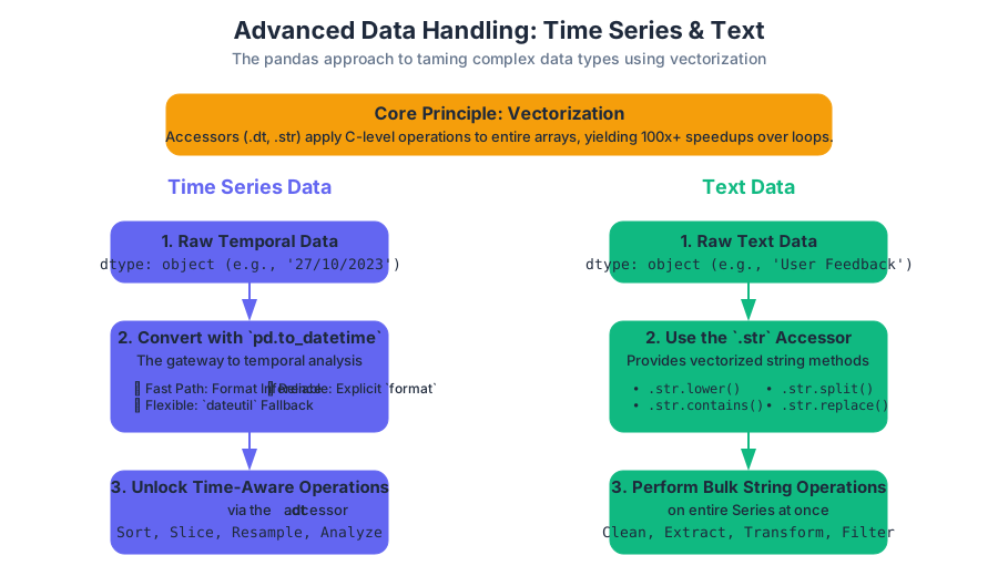
The central theme connecting the handling of both time series and text data in pandas is vectorization. Instead of writing slow, explicit
forloops in Python, we use specialized accessors (.dtand.str) that apply operations to entire arrays of data at the C level. This approach is not merely a convenience; it is a fundamental performance paradigm that can yield speedups of 100x or more, making it possible to process millions of records in seconds.
Time Series Conversion: The Gateway to Temporal Analysis
The journey into time series analysis begins with a crucial first step: converting raw, ambiguous representations of dates and times into a structured, machine-readable format. This is the role of pd.to_datetime.
What it is: pd.to_datetime
pd.to_datetime is a highly optimized and flexible function that parses a wide variety of string, integer, or float representations and converts them into pandas Timestamp objects. A Timestamp is the pandas equivalent of Python's datetime.datetime object but is built upon the more efficient numpy.datetime64[ns] data type, providing nanosecond precision and enabling storage in contiguous memory blocks.
The function is the cornerstone of all time series functionality. Without this explicit conversion, a column of date strings like "2023-10-27" is treated as generic text, sorting lexicographically (e.g., "01-12-2024" would come before "27-10-2023") and prohibiting any form of temporal arithmetic.
Why it matters: Unlocking Time-Aware Operations
Converting data to a datetime format is not just about data typing; it's about unlocking a vast ecosystem of time-aware capabilities. Once converted, data can be:
- Sorted Chronologically: The most fundamental requirement for time series analysis.
- Sliced and Indexed by Date: Selecting data for "October 2023" becomes a trivial operation.
- Used in Temporal Arithmetic: Calculating durations between events (e.g.,
time_to_purchase = purchase_ts - view_ts). - Resampled to Different Frequencies: Aggregating daily data into monthly summaries or vice-versa.
- Analyzed for Seasonality and Trends: Decomposing the timestamp into components like "day of the week" or "quarter of the year".
How it works: Parsing and Inference
Internally, pd.to_datetime employs a multi-layered parsing strategy for both flexibility and speed.
- Format Inference: For array-like inputs, pandas first attempts to infer a common date format. If it finds one (e.g., all strings are in
YYYY-MM-DDformat), it uses a highly optimized, vectorized internal routine to perform the conversion. This is the fastest path. dateutil.parserFallback: If inference fails due to inconsistent or complex formats, pandas falls back to thedateutil.parser.parsefunction for each individual element. This parser is incredibly flexible and can understand formats like"October 27th, 2023", but it is significantly slower as it operates on an element-by-element basis.- Explicit Formatting: The user can provide an explicit format string via the
formatargument (e.g.,format='%d-%m-%Y'). This bypasses inference and thedateutilfallback, guaranteeing the fastest and most reliable parsing path, provided the data is clean.
Concrete Example: From Raw Logs to Datetime Objects
Imagine we have a log file from a web server with timestamps in various, slightly inconsistent formats. Our goal is to parse these into a usable datetime column.
import pandas as pd
import numpy as np

# Raw data with inconsistent formats and an invalid entry
log_data = [
    '2023-10-27 08:30:15',
    '28/10/2023 09:12:05',
    'Oct 29, 2023 11:00:00',
    'Invalid Timestamp',
    '2023-10-30 14:22:30'
]
df = pd.DataFrame(log_data, columns=['raw_timestamp'])

# Convert using pd.to_datetime, coercing errors to NaT (Not a Time)
df['timestamp'] = pd.to_datetime(df['raw_timestamp'], errors='coerce')

# Display the result, showing the parsed datetimes and the NaT
print("--- Parsed Timestamps ---")
print(df)
print("\n--- Data Types ---")
print(df.dtypes)
Output:
--- Parsed Timestamps ---
           raw_timestamp           timestamp
0  2023-10-27 08:30:15 2023-10-27 08:30:15
1  28/10/2023 09:12:05 2023-10-28 09:12:05
2  Oct 29, 2023 11:00:00 2023-10-29 11:00:00
3      Invalid Timestamp                 NaT
4  2023-10-30 14:22:30 2023-10-30 14:22:30

--- Data Types ---
raw_timestamp            object
timestamp        datetime64[ns]
dtype: object
Notice how pd.to_datetime correctly interpreted three different formats and gracefully handled the invalid string by converting it to NaT when errors='coerce' was specified.
In a production pipeline, you might pre-process these logs at the command line before they even enter a Python environment.
# Using awk to attempt to reformat a log file into a consistent ISO 8601 format
# This is a simplified example; a real-world script would be more robust.
# cat server.log | awk '{ ... complex reformatting logic ... }' > cleaned_server.log

# Example: Reformat a DD/MM/YYYY date to YYYY-MM-DD using sed
echo "28/10/2023 09:12:05" | sed -E 's|([0-9]{2})/([0-9]{2})/([0-9]{4})|\3-\2-\1|'
# Output: 2023-10-28 09:12:05
This demonstrates that data cleaning is a multi-stage process, and standardizing formats early can simplify downstream processing in pandas.
Variations / Extensions: Parameterization
The pd.to_datetime function is highly configurable. The table below summarizes its most critical parameters.
| Parameter | Type | Description | Common Use Case |
|---|---|---|---|
arg |
Series, list, str |
The data to be converted. | The primary input data. |
errors |
str |
How to handle parsing errors. 'raise' (default), 'coerce' (set to NaT), 'ignore' (return original input). |
Use 'coerce' for dirty data to avoid script failure. |
format |
str |
The specific strftime format string. |
Massively improves performance on clean, consistent data. |
dayfirst |
bool |
Whether to interpret ambiguous dates like 10/11/12 as DD/MM/YY (True) or MM/DD/YY (False, default). |
Essential when working with European date formats. |
yearfirst |
bool |
Whether to interpret ambiguous dates like 10/11/12 as YY/MM/DD. |
Less common, but useful for certain international formats. |
utc |
bool |
If True, returns a timezone-aware UTC DatetimeIndex. |
Standardizing timestamps from different sources to a single timezone. |
Common Pitfalls
- Timezone Naivety: By default,
pd.to_datetimeproduces timezone-naivedatetimeobjects. This can lead to serious errors when combining data from different geographic locations. Always consider usingtz_localizeto assign a timezone to naive timestamps ortz_convertto switch between timezones. - Performance on Mixed Formats: Relying on the
dateutilfallback for millions of rows with inconsistent formats will be a major performance bottleneck. The best practice is to clean and standardize date strings as much as possible before callingpd.to_datetime, and then use theformatargument.
The Datetime Accessor: Decomposing Time
Once a Series is of datetime64 type, you gain access to the .dt accessor. This powerful tool is the key to feature engineering from temporal data.
What it is: The .dt Accessor
The .dt accessor is a special property available on pandas Series that contain datetime-like values. It exposes a wide range of properties and methods for extracting temporal components in a vectorized manner. For example, series.dt.year returns a new Series containing the year of each timestamp.
Why it matters: Feature Engineering from Time
A raw timestamp like 2023-10-27 08:30:15.123456789 is a high-cardinality feature that is nearly useless to most machine learning models. Its value is in its components. By decomposing it, we can create meaningful features that capture patterns and seasonality:
- Is there a difference in user activity on weekends vs. weekdays? (
.dt.weekdayor.dt.day_name()) - Do sales peak in the last month of the quarter? (
.dt.month,.dt.quarter) - Is there a specific hour of the day when server load is highest? (
.dt.hour)
The .dt accessor makes creating these features trivial and computationally efficient.
Concrete Example: Analyzing User Login Patterns
Let's analyze a dataset of user login timestamps to identify the busiest days of the week and hours of the day.
# Generate a realistic series of 10,000 login timestamps over a month
rng = np.random.default_rng(0)
base_time = pd.to_datetime('2023-10-01')
random_seconds = rng.integers(0, 30*24*3600, size=10000)
login_timestamps = base_time + pd.to_timedelta(random_seconds, unit='s')
logins = pd.Series(login_timestamps, name='login_time').sort_values()

# --- Feature Engineering with .dt accessor ---
df = pd.DataFrame(logins)
df['day_of_week'] = df['login_time'].dt.day_name()
df['hour_of_day'] = df['login_time'].dt.hour

# --- Analysis ---
# Find the busiest hour of the day
busiest_hour = df['hour_of_day'].value_counts().nlargest(1)
print(f"Busiest hour of the day:\n{busiest_hour}\n")

# Find the busiest day of the week
day_order = ["Monday", "Tuesday", "Wednesday", "Thursday", "Friday", "Saturday", "Sunday"]
busiest_day = df['day_of_week'].value_counts().loc[day_order]
print(f"Logins by day of the week:\n{busiest_day}")
Output:
Busiest hour of the day:
hour_of_day
18    453
Name: count, dtype: int64

Logins by day of the week:
day_of_week
Monday       1403
Tuesday      1429
Wednesday    1433
Thursday     1407
Friday       1469
Saturday     1447
Sunday       1412
Name: count, dtype: int64
This example shows a complete mini-analysis: we took raw timestamps, used .dt to engineer meaningful categorical features, and then used standard pandas methods like .value_counts() to derive insights.
Variations / Extensions: The Breadth of .dt Properties
The .dt accessor provides a rich set of attributes.
| Property/Method | Returns | Description |
|---|---|---|
.year, .month, .day |
int |
The corresponding integer value for the date component. |
.hour, .minute, .second |
int |
The corresponding integer value for the time component. |
.weekday |
int |
The day of the week, where Monday=0 and Sunday=6. |
.day_name() |
str |
The full name of the day (e.g., "Monday"). |
.month_name() |
str |
The full name of the month (e.g., "October"). |
.quarter |
int |
The quarter of the year (1-4). |
.is_month_start |
bool |
True if the date is the first day of the month. |
.is_year_end |
bool |
True if the date is the last day of the year. |
.strftime('%Y-%m-%d') |
str |
Formats the datetime back into a string with a custom format. |
.round('H') |
datetime |
Rounds the timestamp to the nearest specified frequency (e.g., hour). |
The DatetimeIndex: Supercharging Selection and Slicing
While the .dt accessor operates on Series, the true power of pandas time series is realized when a datetime column is set as the DataFrame's index, creating a DatetimeIndex.
What it is: A Time-Based Index
A DatetimeIndex is a specialized pandas Index object composed of Timestamp objects. It is optimized for time-based data access and alignment. You can create one by passing a datetime Series to df.set_index().
Why it matters: Intuitive and Efficient Time-Based Queries
A DatetimeIndex revolutionizes how you select data. Instead of complex boolean filtering like df[(df['date'] >= '2023-10-01') & (df['date'] < '2023-11-01')], you can use concise, intuitive string-based slicing.
Key Insight:
DatetimeIndexenables label-based slicing with partial date strings.df['2023']selects all data for the year 2023.df['2023-10']selects all data for October 2023. This is not just syntactic sugar; it's a gateway to high-performance time-window queries.
How it works: Under the Hood
The performance of DatetimeIndex comes from its underlying structure. It is backed by a monotonic numpy.datetime64[ns] array. When you perform a slice like df['2023-10-01':'2023-10-15'], pandas doesn't need to scan every row. Because the index is sorted, it can use efficient search algorithms (like binary search) to quickly locate the start and end positions of the slice, making lookups extremely fast, often O(log N).
Concrete Example: Slicing Financial Stock Data
Consider a DataFrame of daily stock prices indexed by date.
# Create a sample DataFrame with a DatetimeIndex
dates = pd.date_range(start='2023-01-01', end='2023-12-31', freq='D')
data = {
    'price': 100 + np.random.randn(len(dates)).cumsum(),
    'volume': np.random.randint(1_000_000, 5_000_000, size=len(dates))
}
stocks_df = pd.DataFrame(data, index=dates)
stocks_df.index.name = 'date'

print("--- Original DataFrame Head ---")
print(stocks_df.head())

# --- Slicing Examples ---

# 1. Select a single day's data
print("\n--- Data for October 27, 2023 ---")
print(stocks_df.loc['2023-10-27'])

# 2. Select an entire month (October 2023)
print("\n--- Data for October 2023 ---")
october_data = stocks_df['2023-10']
print(october_data.head(2))
print(october_data.tail(2))

# 3. Select a specific date range (first two weeks of Q4)
print("\n--- Data for Q4 Start (Oct 1 to Oct 14, 2023) ---")
q4_start = stocks_df.loc['2023-10-01':'2023-10-14']
print(q4_start)
AI_DEMOI_DEMOhis code demonstrates the elegance and power of DatetimeIndex slicing. The syntax is clean, readable, and internally optimized for performance.
Time Frequency Resampling: Aggregating and Interpolating
Resampling is the process of converting a time series from one frequency to another. It is a fundamental operation for summarizing data, aligning disparate datasets, and filling in missing values.
What it is: The .resample() Method
The .resample() method is a time-based groupby operation. It is called on a Series or DataFrame with a DatetimeIndex and is immediately followed by an aggregation (.sum(), .mean(), .ohlc()) or interpolation (.asfreq(), .ffill()) method.
There are two primary types of resampling:
- Downsampling: Aggregating data from a high frequency to a low frequency (e.g., daily data to monthly data). This reduces the number of rows and requires an aggregation function to combine the data points within each new period (e.g.,
sum()of daily sales to get monthly sales). - Upsampling: Converting data from a low frequency to a high frequency (e.g., daily data to hourly data). This increases the number of rows and introduces missing values, which must be filled using a method like forward-fill (
.ffill()) or interpolation (.interpolate()).
Why it matters: Aligning and Summarizing Data
Resampling is critical for:
- Creating Reports: Generating quarterly or annual summaries from daily operational data.
- Noise Reduction: Smoothing out volatile, high-frequency data to reveal underlying trends.
- Data Alignment: Aligning two datasets with different frequencies (e.g., daily sales and weekly marketing spend) before modeling their relationship.
How it works: The Split-Apply-Combine Paradigm
The .resample() method follows the classic "split-apply-combine" pattern:
- Split: The
DatetimeIndexis conceptually divided into time bins according to the target frequency (e.g., for.resample('M'), all data points from October 1st to October 31st fall into the "October" bin). - Apply: An aggregation function is applied to the data within each bin. For example,
.mean()calculates the average of all values in that bin. - Combine: The results of the aggregation for each bin are collected into a new Series or DataFrame, indexed by the end (or start) of each time bin.
Concrete Example: From Daily Sales to Monthly Totals
Let's downsample a daily sales dataset to get a monthly summary.
# Using the stocks_df from the previous example, let's treat 'volume' as 'daily_sales'
sales_df = stocks_df[['volume']].rename(columns={'volume': 'daily_sales'})

# Resample daily sales to monthly totals
# 'M' stands for month-end frequency
monthly_sales = sales_df.resample('M').sum()
print("--- Monthly Sales Totals (Sum) ---")
print(monthly_sales)

# Resample to quarterly averages
# 'Q' stands for quarter-end frequency
quarterly_avg_sales = sales_df.resample('Q').mean()
print("\n--- Quarterly Average Daily Sales ---")
print(quarterly_avg_sales)
Output:
--- Monthly Sales Totals (Sum) ---
            daily_sales
date
2023-01-31     93333939
2023-02-28     83196887
2023-03-31     93175891
...
2023-12-31     92900983

--- Quarterly Average Daily Sales ---
                 daily_sales
date
2023-03-31      3.000064e+06
2023-06-30      2.990425e+06
2023-09-30      3.007687e+06
2023-12-31      3.021021e+06
This is a standard operation in business intelligence. The equivalent operation in SQL would use a date truncation function.
-- SQL equivalent for calculating monthly total sales
SELECT
  DATE_TRUNC('month', sale_date) AS month,
  SUM(sales_amount) AS total_sales
FROM
  sales
GROUP BY
  DATE_TRUNC('month', sale_date)
ORDER BY
  month;
This comparison highlights how .resample() provides a concise, powerful syntax for a common and critical database operation.
Vectorized String Operations: The .str Accessor
Just as the .dt accessor unlocks temporal data, the .str accessor is the key to processing textual data efficiently.
What it is: The .str Accessor
The .str accessor is a property on pandas Series with object dtype (typically containing strings) that exposes vectorized versions of Python's standard string methods. This allows you to apply string manipulations to an entire Series at once, without writing an explicit Python loop.
Why it matters: Avoiding Slow Python Loops
The performance difference between a vectorized .str operation and a Python loop is staggering.
# Performance comparison: Vectorized vs. Loop
import timeit

s = pd.Series(['string ' * 5] * 10000)

# Vectorized approach
vector_time = timeit.timeit(lambda: s.str.upper().str.strip(), number=100)

# Loop-based approach (using .apply with a lambda)
loop_time = timeit.timeit(lambda: s.apply(lambda x: x.upper().strip()), number=100)

print(f"Vectorized (.str) time: {vector_time:.4f} seconds")
print(f"Loop (.apply) time:     {loop_time:.4f} seconds")
print(f"Speedup: {loop_time / vector_time:.1f}x")

# On a typical machine, this will show a 10-50x speedup for the vectorized version.
This is because .str methods operate on the data at a lower level (often in C), avoiding the significant overhead of the Python interpreter for each element in the Series.
Concrete Example: Cleaning User-Entered Data
A common task is cleaning inconsistent text fields, such as product names entered by users.
# Messy product names
products = pd.Series([
    '  Product A ', 'product b', ' PRODUCT C', np.nan, 'Product_D'
])

# Chained .str methods for cleaning
cleaned_products = (
    products
    .str.strip()          # Remove leading/trailing whitespace
    .str.lower()          # Convert to lowercase
    .str.replace('_', ' ') # Replace underscores with spaces
)

print("--- Before Cleaning ---")
print(products)
print("\n--- After Cleaning ---")
print(cleaned_products)
Output:
--- Before Cleaning ---
0      Product A
1        product b
2       PRODUCT C
3             NaN
4       Product_D
dtype: object

--- After Cleaning ---
0    product a
1    product b
2    product c
3          NaN
4    product d
dtype: object
Note how NaN values are gracefully propagated through the chain of operations, which is the desired behavior in most data cleaning pipelines.
String Splitting and Filtering
Beyond simple cleaning, the .str accessor provides powerful methods for splitting strings into multiple columns and filtering rows based on complex patterns, often using regular expressions.
What it is: Pattern Matching and Extraction
This category includes methods like:
.str.contains(pat): Returns a booleanSeriesindicating if the patternpatis found in each string..str.split(pat, expand=True): Splits each string by the patternpatand expands the results into a new DataFrame..str.extract(pat): Uses a regular expression with capturing groups to extract substrings into new columns in a DataFrame.
Why it matters: Structuring Unstructured Text
These methods are the workhorses for converting semi-structured text into a fully structured, tabular format. A log entry like "ERROR:DB-01:Connection timed out" is not easily analyzable until it is split into Level, Source, and Message columns.
How it works: Regular Expressions as a First-Class Citizen
The true power of these methods is unlocked by regular expressions (regex). By setting regex=True (the default for many methods), you can define sophisticated patterns for matching and extraction.
.str.contains()becomes a powerful filter for finding records that match a complex rule..str.split(expand=True)is the fastest way to break apart delimited data..str.extract()is surgical. It uses parentheses()in the regex pattern to define capturing groups. Each group becomes a new column in the output DataFrame, containing only the text that matched that part of the pattern.
Concrete Example: Parsing Server Log Entries
Let's parse a Series of log entries to filter for errors and extract structured information.
logs = pd.Series([
    'INFO:2023-10-27:192.168.1.1:User logged in successfully',
    'WARN:2023-10-27:192.168.1.1:Login attempt failed',
    'ERROR:2023-10-28:10.0.0.5:Database connection failed: timeout',
    'INFO:2023-10-28:192.168.1.2:File uploaded'
])
df = pd.DataFrame({'log_entry': logs})

# 1. Filter for only ERROR messages
error_logs = df[df['log_entry'].str.contains('^ERROR')]
print("--- Error Logs Only ---")
print(error_logs)

# 2. Split the log entry into structured columns
# We use .str.split with a limit (n=3) to avoid splitting the message itself
log_parts = df['log_entry'].str.split(':', n=3, expand=True)
log_parts.columns = ['level', 'date', 'ip_address', 'message']
print("\n--- Parsed Log DataFrame ---")
print(log_parts)
Output:
--- Error Logs Only ---
                                           log_entry
2  ERROR:2023-10-28:10.0.0.5:Database connection ...

--- Parsed Log DataFrame ---
   level        date  ip_address                       message
0   INFO  2023-10-27  192.168.1.1  User logged in successfully
1   WARN  2023-10-27  192.168.1.1         Login attempt failed
2  ERROR  2023-10-28    10.0.0.5   Database connection failed: timeout
3   INFO  2023-10-28  192.168.1.2                 File uploaded
For more complex extraction, like pulling a username and action from a message, .str.extract() is superior. Consider a regex for a different log format.
# A regex to parse an Apache common log format entry
# It has capturing groups for IP, timestamp, request, status, and size.
^(\S+) \S+ \S+ \[(.*?)\] "(\S+ \S+ \S+)" (\d{3}) (\d+)$
Using this pattern with .str.extract() on Apache logs would instantly produce a structured DataFrame with five columns, a task that would be incredibly tedious and slow using manual string processing.
Common Pitfalls
- Greedy Regex: A common regex mistake is a "greedy" pattern like
.*that matches more than intended. Use non-greedy.*?or more specific character classes. - Performance of Complex Regex: While much faster than Python loops, a poorly written, inefficient regex can still be slow on very large datasets. Test and profile your patterns.
- Forgetting
expand=True: A call to.str.split()withoutexpand=Truereturns aSeriesof lists, which is often less useful than the DataFrame produced when it is set toTrue.
Comparing pandas with Other Data Tools
Key concepts: Comparison with R (dplyr) · Comparison with SQL (SELECT, WHERE, GROUP BY) · Comparison with Spreadsheets · Comparison with SAS/Stata/SPSS · Terminology Mapping · Syntax Translation
A translation guide for users familiar with other data analysis tools like R, SQL, SAS, and spreadsheets. This section maps common operations and terminology from those environments to their pandas equivalents, accelerating the learning curve for experienced analysts.
Comparing pandas with Other Data Tools
For practitioners transitioning to Python's data science ecosystem, the pandas library often serves as the primary gateway. Its power lies in providing expressive, high-performance data structures and analysis tools. However, its concepts are not entirely novel; they are a powerful synthesis and evolution of ideas from many preceding data analysis environments. Understanding these parallels is the fastest way to master pandas, as it allows you to map existing mental models onto its API. This section serves as a Rosetta Stone, translating the paradigms of SQL, R, spreadsheets, and traditional statistical software into the language of pandas.
AI_SVGI_SVG## Comparison with SQL
The most direct and powerful analogy for pandas is with Structured Query Language (SQL). Both are designed for relational, or tabular, data manipulation. While SQL is a declarative language for querying databases, pandas provides a programmatic, imperative interface for in-memory data transformation. The core relational algebra operations—selection, projection, join, and aggregation—have direct equivalents.
Key Insight: Think of a pandas DataFrame as a single database table that you have loaded into memory. The pandas API provides the tools to perform all the queries you would normally run against that table using SQL.
Terminology and Syntax Mapping
The fundamental operations in SQL map cleanly to pandas methods. This one-to-one correspondence is the cornerstone of translating data manipulation logic between the two systems.
| SQL Concept | SQL Syntax | pandas Equivalent | Description |
|---|---|---|---|
| Projection | SELECT col1, col2 FROM table |
df[['col1', 'col2']] |
Selecting a subset of columns. |
| Selection / Filtering | SELECT * FROM table WHERE col1 > 10 |
df[df['col1'] > 10] or df.query('col1 > 10') |
Selecting a subset of rows based on a condition. |
| Aggregation | SELECT AGG(col) FROM table GROUP BY grp |
df.groupby('grp')['col'].agg() |
Applying a function (e.g., SUM, MEAN) to groups of rows. |
| Join | SELECT * FROM t1 JOIN t2 ON t1.key = t2.key |
pd.merge(df1, df2, on='key') |
Combining data from multiple tables based on a common key. |
| Sorting | SELECT * FROM table ORDER BY col DESC |
df.sort_values('col', ascending=False) |
Ordering rows based on the values in one or more columns. |
| Limiting Results | SELECT * FROM table LIMIT 10 |
df.head(10) |
Selecting the first N rows. |
| Distinct Values | SELECT DISTINCT col FROM table |
df['col'].unique() |
Finding the unique values in a column. |
Concrete Example: A Multi-Step Query
Let's consider a realistic business query: "Find the top 3 product categories by total sales for customers in North America who registered after 2022."
This requires joining tables, filtering, grouping, aggregating, and sorting.
Here is the standard SQL approach, assuming a database with sales, customers, and products tables.
-- SQL: A complete query to find top-selling categories for a customer segment
SELECT
    p.category,
    SUM(s.quantity * s.price_per_unit) AS total_sales
FROM
    sales s
JOIN
    customers c ON s.customer_id = c.customer_id
JOIN
    products p ON s.product_id = p.product_id
WHERE
    c.region = 'North America'
    AND c.registration_date >= '2022-01-01'
GROUP BY
    p.category
ORDER BY
    total_sales DESC
LIMIT 3;
Now, let's translate this entire workflow into a pandas method chain. Assume we have three DataFrames: sales_df, customers_df, and products_df.
# Python/pandas: The equivalent data manipulation pipeline
import pandas as pd

# Assume sales_df, customers_df, products_df are already loaded
# e.g., sales_df = pd.read_csv('sales.csv')

# 1. First, perform the joins (merges)
merged_df = pd.merge(sales_df, customers_df, on='customer_id')
full_df = pd.merge(merged_df, products_df, on='product_id')

# 2. Apply filters
filtered_df = full_df[
    (full_df['region'] == 'North America') &
    (pd.to_datetime(full_df['registration_date']) >= '2022-01-01')
]

# 3. Create the total sales column
filtered_df['total_sales'] = filtered_df['quantity'] * filtered_df['price_per_unit']

# 4. Group by category, aggregate, sort, and get the top 3
top_categories = (
    filtered_df.groupby('category')['total_sales']
    .sum()
    .sort_values(ascending=False)
    .head(3)
)

print(top_categories)
Common Pitfalls
NULLvs.NaN: SQL usesNULLto represent missing data, which has specific three-valued logic. Pandas usesnp.nan(Not a Number), a floating-point value with different semantics. For example,np.nan == np.nanisFalse, whereasNULL = NULLisNULLin SQL. This can lead to subtle differences in filtering and joins.- Performance: SQL databases are highly optimized for disk-based, out-of-core operations and can leverage sophisticated query planners and indexes. Pandas operates entirely in-memory. For datasets that fit comfortably in RAM, pandas can be significantly faster. For datasets that exceed available RAM, database solutions are superior.
- Mutability: SQL queries on a database are typically read-only operations that produce a new result set. In pandas, operations can either return a new DataFrame (e.g.,
merge) or modify an existing one in-place (e.g., usinginplace=True, though this is now discouraged). Managing this state is a key difference in the programming model.
Comparison with R (dplyr)
For users coming from the R ecosystem, the most relevant comparison is with the dplyr package, part of the Tidyverse. dplyr provides a "grammar of data manipulation" centered on a small set of verbs that can be combined to solve complex problems. Pandas, while not explicitly designed with this grammar, has a very similar set of capabilities that can be chained together to achieve the same expressive power.
A Grammar-Based Mapping
The core idea of dplyr is to use pipes (%>% or |>) to chain together single-purpose functions. The pandas equivalent is method chaining, where each method call returns a DataFrame, which is then used by the next method in the chain.
dplyr Verb |
R (dplyr) Syntax | pandas Equivalent | Description |
|---|---|---|---|
filter() |
df %>% filter(col > 10) |
df[df['col'] > 10] or df.query('col > 10') |
Keep rows that satisfy a condition. |
select() |
df %>% select(col1, col2) |
df[['col1', 'col2']] |
Pick columns by name. |
mutate() |
df %>% mutate(new_col = col1 * 2) |
df.assign(new_col = lambda x: x['col1'] * 2) |
Create new columns. |
arrange() |
df %>% arrange(desc(col)) |
df.sort_values('col', ascending=False) |
Reorder rows. |
summarise() |
df %>% summarise(avg = mean(col)) |
df.agg(avg=('col', 'mean')) |
Reduce variables to values. |
group_by() |
df %>% group_by(grp) |
df.groupby('grp') |
Perform operations by group. |
Concrete Example: A Data Tidying Pipeline
Let's replicate a common data analysis task: for a dataset of flight delays, find the average arrival and departure delay for each airline carrier, sorted by the arrival delay.
Here is the elegant and readable dplyr implementation.
# R/dplyr: A typical data analysis pipeline
library(dplyr)
library(nycflights13)

# Find the average delay per carrier, sorted by arrival delay
carrier_delays <- flights %>%
  group_by(carrier) %>%
  summarise(
    avg_arr_delay = mean(arr_delay, na.rm = TRUE),
    avg_dep_delay = mean(dep_delay, na.rm = TRUE),
    n = n()
  ) %>%
  filter(n > 1000) %>% # Only consider carriers with a significant number of flights
  arrange(desc(avg_arr_delay))

print(head(carrier_delays))
The equivalent pandas code uses method chaining to achieve a similar flow and readability.
# Python/pandas: The same pipeline using method chaining
import pandas as pd
# Assume 'flights' is a DataFrame loaded from a CSV or other source

carrier_delays = (
    flights
    .groupby('carrier')
    .agg(
        avg_arr_delay=('arr_delay', 'mean'),
        avg_dep_delay=('dep_delay', 'mean'),
        n=('carrier', 'size') # 'size' is equivalent to dplyr's n()
    )
    .query('n > 1000') # Using query for a more dplyr-like filter
    .sort_values('avg_arr_delay', ascending=False)
)

print(carrier_delays.head())
Variations and Extensions
- The
pipe()Method: For functions that are not DataFrame methods, pandas provides a.pipe()method to maintain the chain. This is useful for applying complex, custom transformations. siuba: For those who truly prefer thedplyrsyntax, the Python librarysiubaprovides a direct port ofdplyr's grammar that operates on pandas DataFrames, offering a "best of both worlds" approach.
Common Pitfalls
- Indexing: R is 1-indexed, while Python (and pandas) is 0-indexed. This is a fundamental difference that often trips up new users, especially when using positional selection with
.iloc. - Vectorization vs.
.apply(): R's functions are generally vectorized by default. In pandas, while most core operations are vectorized (and extremely fast), users sometimes fall back on.apply()with a Python function for custom logic. This is often much slower than finding a native, vectorized pandas solution. - Data Type Handling: R's
factortype for categorical data has different behaviors from pandas'Categorydtype, especially concerning ordering and available methods.
Comparison with Spreadsheets
For millions of users, the spreadsheet (e.g., Microsoft Excel, Google Sheets) is the primary tool for data analysis. While incredibly accessible, spreadsheets suffer from issues with reproducibility, scalability, and error-proneness. Pandas provides a programmatic and robust alternative to spreadsheet-based workflows.
Key Insight: A pandas DataFrame is a programmatic representation of a spreadsheet worksheet. A Series is a column. Instead of clicking and dragging, you write code to manipulate the data, which makes your analysis transparent, repeatable, and scalable.
Conceptual Mapping
| Spreadsheet Concept | pandas Equivalent | Description |
|---|---|---|
| Worksheet / Tab | DataFrame |
A 2D table of data. |
| Column | Series |
A 1D array of data, representing a single column. |
| Cell Formula | Vectorized Operation | Applying a formula to an entire column at once (e.g., df['C'] = df['A'] + df['B']). |
| VLOOKUP / XLOOKUP | pd.merge() or Series.map() |
Looking up values from one table and adding them to another based on a common key. |
| Pivot Table | df.pivot_table() |
Reshaping and summarizing data by grouping on one or more columns. |
| Filtering | Boolean Indexing | Hiding or showing rows based on cell values. |
| Sorting | df.sort_values() |
Rearranging rows based on column values. |
Concrete Example: From VLOOKUP to merge
Imagine you have a sales table in one sheet and a product details table in another. In Excel, you would use VLOOKUP to bring the product category into the sales sheet.
=VLOOKUP(B2, Products!A:B, 2, FALSE)
This formula, dragged down a column, looks up the product_id from cell B2 in the Products sheet and returns the corresponding category.
In pandas, this operation is a left merge. It is more explicit, robust, and handles multiple matching keys or data type issues more gracefully.
# Python/pandas: Replicating a VLOOKUP with a left merge
import pandas as pd

sales = pd.DataFrame({
    'transaction_id': [101, 102, 103, 104],
    'product_id': ['P01', 'P02', 'P01', 'P03'],
    'quantity': [5, 2, 8, 3]
})

products = pd.DataFrame({
    'id': ['P01', 'P02', 'P03'],
    'category': ['Electronics', 'Books', 'Home Goods'],
    'supplier': ['Supplier A', 'Supplier B', 'Supplier A']
})

# The merge operation is the VLOOKUP equivalent
sales_with_category = pd.merge(
    sales,
    products,
    left_on='product_id',
    right_on='id',
    how='left' # 'left' ensures all sales records are kept
)

print(sales_with_category)
# The 'id' column from the products table can be dropped if not needed
# sales_with_category.drop('id', axis=1, inplace=True)
AI_DEMOI_DEMO### Common Pitfalls
- Paradigm Shift: The biggest hurdle is moving from a visual, cell-based, direct manipulation model to a programmatic, abstract, column-based model. In Excel, you "see" your data change. In pandas, you execute code that transforms an abstract data structure.
- Data Integrity: Spreadsheets often have mixed data types within a single column (e.g., numbers and text strings representing errors). Pandas enforces a single
dtypeper column, which is stricter but ensures data integrity and computational efficiency. This often requires significant data cleaning when importing from Excel. - Scalability: A common workflow is to perform initial analysis in Excel until the dataset grows too large (e.g., >1 million rows), at which point the application becomes slow or crashes. Migrating to pandas at this stage can be challenging. Learning pandas from the start avoids this scalability cliff.
Comparison with Statistical Software (SAS/Stata/SPSS)
For decades, statistical packages like SAS, Stata, and SPSS have been the industry standard in fields like biostatistics, econometrics, and social sciences. These tools are powerful, well-validated, and have a rich history. However, they are often domain-specific, proprietary, and operate under a different programming paradigm than general-purpose languages like Python.
Procedural vs. Object-Oriented Paradigm
The core difference is the programming model.
- SAS/Stata/SPSS are largely procedural. The user writes a series of commands or procedures that operate on a global dataset (e.g., the SAS
WORKlibrary).DATAsteps are used for manipulation, andPROC(procedure) steps are used for analysis. - pandas is object-oriented. The data is encapsulated in an object (the DataFrame), and the user calls methods on that object. This allows for multiple datasets to be held in memory simultaneously and for more modular, reusable code.
Terminology and Command Mapping
| SAS/Stata Concept | SAS/Stata Syntax | pandas Equivalent | Description |
|---|---|---|---|
| Data Step | DATA new; SET old; new_var=...; RUN; |
df['new_var'] = ... |
Creating and modifying variables. |
| Procedure (PROC) | PROC MEANS; VAR x; RUN; |
df['x'].describe() |
Running a statistical analysis. |
| Keep/Drop Statement | KEEP var1 var2; |
df[['var1', 'var2']] |
Selecting columns. |
| Where Statement | WHERE condition; |
df[df['col'] == condition] |
Filtering rows. |
| By-Group Processing | BY group_var; |
df.groupby('group_var') |
Performing analysis on subgroups. |
| Proc Freq | PROC FREQ; TABLES var; RUN; |
df['var'].value_counts() |
Frequency counts for a categorical variable. |
Concrete Example: Basic Data Summary
Let's perform a simple task: in a dataset, create a binary variable based on a continuous one, and then calculate mean statistics for a third variable, grouped by our new binary variable.
Here is a typical SAS program for this task.
* SAS: A classic DATA step followed by a PROC step;
DATA titanic_with_agegroup;
    SET mylib.titanic; /* Assume titanic dataset is in mylib library */
    IF age < 18 THEN is_child = 1;
    ELSE is_child = 0;
RUN;

PROC MEANS DATA=titanic_with_agegroup N MEAN STD;
    CLASS is_child;
    VAR fare;
RUN;
This code first creates a new dataset with the is_child variable, then runs the MEANS procedure on it. The pandas equivalent is more compact and fluid.
# Python/pandas: The object-oriented equivalent
import pandas as pd
import numpy as np

# Assume 'titanic' is a DataFrame
# Create the new column using a vectorized function like np.where
titanic['is_child'] = np.where(titanic['age'] < 18, 1, 0)

# Perform the by-group analysis
fare_summary = titanic.groupby('is_child')['fare'].agg(['count', 'mean', 'std'])

print(fare_summary)
Common Pitfalls
- Ecosystem Integration: SAS and Stata are often all-in-one environments. In Python, pandas is just one piece of a larger ecosystem. You use
pandasfor manipulation,statsmodelsorscikit-learnfor modeling,matplotliborseabornfor plotting, andJupyterfor interactive analysis. This modularity is powerful but requires learning how the different libraries interact. - Cost and Licensing: SAS/Stata/SPSS are commercial products with significant licensing fees. The Python ecosystem is entirely open-source and free.
- Out-of-Core Processing: SAS, in particular, is renowned for its ability to process massive datasets that do not fit in memory by efficiently managing temporary files on disk. While libraries like Dask provide this capability for pandas-like DataFrames in Python, it is not a built-in feature of pandas itself and requires a different approach.
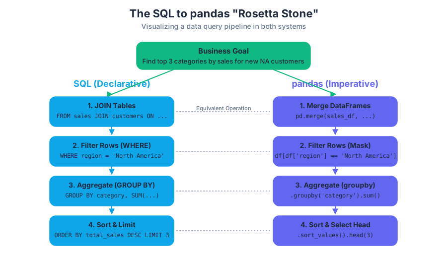
Essential Guides and References
Key concepts: User Guide · API Reference · Cheat Sheet · Data Structures · Indexing and Selecting Data
A curated list of the most important guides and reference materials for both quick lookups and in-depth learning. This section points you to the comprehensive User Guide, a fast-paced '10 minutes' tutorial, and a handy cheat sheet.
Essential Guides and References
Navigating a library as comprehensive as pandas requires more than just memorizing function names; it demands a strategic understanding of its documentation and a firm grasp of its core conceptual model. While tutorials provide an initial on-ramp, true proficiency is built by knowing how to find answers and why the library is designed the way it is. This guide moves beyond introductory steps to dissect the essential reference materials and foundational concepts—data structures and indexing—that form the bedrock of all data manipulation in pandas. Mastering these is the critical transition from following recipes to composing your own sophisticated data analysis solutions.
AI_SVGI_SVG## The Canonical Documentation Trio
The pandas documentation is vast, but it can be navigated effectively by understanding the distinct purpose of its three primary resources: the User Guide, the API Reference, and the community Cheat Sheet. Treating them as interchangeable is a common mistake; recognizing their specific roles will dramatically accelerate your learning and problem-solving.
| Resource | Purpose | Best For | Analogy |
|---|---|---|---|
| User Guide | Thematic, conceptual explanations | Understanding how and why a feature works; learning a new topic area from first principles. | A textbook or a series of lectures. |
| API Reference | Precise, exhaustive function specifications | Finding the exact signature, parameters, and return value of a specific function you already know. | A dictionary or an encyclopedia. |
| Cheat Sheet | High-density, quick-reference syntax | Reminding yourself of the syntax for a common, everyday operation. | A set of flashcards or a pilot's checklist. |
User Guide: The Thematic Deep Dive
The User Guide is the narrative heart of the pandas documentation. It is organized by topic, not by function name, and is designed to be read section by section. When you want to understand a concept like "grouping," "time series," or "reshaping" in its entirety, the User Guide is your definitive source. It explains the motivation behind features, illustrates them with detailed examples, and connects them to other parts of the library.
Key Insight: Always start with the User Guide when you are trying to accomplish a new type of task. For example, if you need to combine two datasets but are unsure of the best method, the "Merge, join, concatenate and compare" section of the User Guide will explain the trade-offs between
pd.merge(),pd.concat(), and.join(), guiding you to the correct choice. The API reference, in contrast, assumes you already know which function you need.
API Reference: The Precise Specification
The API Reference is the library's technical blueprint. It is an exhaustive, alphabetically organized list of every public class, method, and function in pandas. Each entry provides the exact function signature, a detailed description of every parameter, information about what the function returns, and often, simple, self-contained examples.
You should turn to the API Reference when you have a specific question about a function's behavior:
- "What are all the possible values for the
howparameter inpd.merge()?" - "Does the
.dropna()method operate in-place by default?" - "What is the exact data type of the object returned by
.groupby()?"
Searching the API Reference for conceptual guidance is inefficient. It's a tool for precision, not exploration.
Cheat Sheet: The Quick-Access Map
The pandas Cheat Sheet, typically a two-page PDF, is an invaluable desktop companion. It provides no conceptual explanation but offers a dense visual summary of the syntax for the most common 80% of data manipulation tasks. It's organized visually by task (e.g., Reshaping Data, Subsetting Data), making it perfect for those "how do I do that again?" moments. It serves as an external memory aid, jogging your recall of syntax you've learned but may not use every day.
Core Abstractions: The DataFrame and Series
At the heart of pandas are two fundamental data structures: the DataFrame and the Series. Understanding their properties and relationship is non-negotiable for effective use of the library.
What They Are
A
Seriesis a one-dimensional, labeled array capable of holding data of any single NumPy data type (integers, strings, floating-point numbers, Python objects, etc.). The labels are collectively referred to as the index.A
DataFrameis a two-dimensional, size-mutable, and potentially heterogeneous tabular data structure with labeled axes (rows and columns). You can think of it as a dictionary-like container forSeriesobjects, where eachSeriesrepresents a column.
A DataFrame has both a row index and a column index. A Series has only a row index. The Name attribute of a Series often corresponds to the column name it would have in a DataFrame.
Why They Matter
These structures solve critical problems that are cumbersome to handle with other tools. A NumPy array is powerful but requires homogeneous data—all elements must be of the same type. A standard Python dictionary of lists is flexible but lacks the performance, alignment features, and rich analytical methods required for serious data work.
The pandas DataFrame and Series provide the best of both worlds:
- Performance: Operations are vectorized, leveraging NumPy and C/Cython implementations under the hood for speeds far exceeding native Python loops.
- Data Alignment: Operations between
SeriesorDataFrameobjects automatically align on their index labels. This prevents subtle, off-by-one errors common in manual data manipulation and is a cornerstone of pandas' power. - Rich Functionality: They come with a vast, integrated library of methods for data cleaning, transformation, aggregation, and visualization.
How They Work
Internally, a DataFrame is not just a simple 2D array. It's a more complex object that manages a collection of 1D arrays (typically NumPy arrays), one for each column. This column-oriented design is called a BlockManager. It groups columns of the same data type into "blocks" (e.g., a block for all float64 columns, a block for all int64 columns, a block for object columns). This allows for efficient storage and computation, as vectorized operations can be applied to entire blocks of homogeneous data at once.
Here is a simplified, conceptual implementation in Python to illustrate the core idea of a DataFrame as a manager of aligned, named Series.
import numpy as np

class SimpleSeries:
    """A conceptual, simplified implementation of a pandas Series."""
    def __init__(self, data, index=None, name=None):
        if not isinstance(data, np.ndarray):
            data = np.array(data)
        if index is None:
            index = np.arange(len(data))

        if len(data) != len(index):
            raise ValueError("Data and index must be of the same length.")

        self.data = data
        self.index = np.array(index)
        self.name = name

    def __repr__(self):
        output = ""
        for idx, val in zip(self.index, self.data):
            output += f"{idx}\t{val}\n"
        output += f"Name: {self.name}, dtype: {self.data.dtype}"
        return output

    def __len__(self):
        return len(self.data)

class SimpleDataFrame:
    """A conceptual, simplified implementation of a pandas DataFrame."""
    def __init__(self, data_dict):
        # Ensure all inputs are list-like and have the same length
        first_key = next(iter(data_dict))
        self._length = len(data_dict[first_key])

        self._columns = list(data_dict.keys())
        self._data = {}

        for col_name, col_data in data_dict.items():
            if len(col_data) != self._length:
                raise ValueError("All columns must have the same length.")
            # Internally, this would be a more complex BlockManager
            self._data[col_name] = np.array(col_data)

        self.index = np.arange(self._length)

    def __repr__(self):
        header = "\t" + "\t".join(self._columns) + "\n"
        body = ""
        for i in self.index:
            row_vals = [str(self._data[col][i]) for col in self._columns]
            body += f"{i}\t" + "\t".join(row_vals) + "\n"
        return header + body

# Usage
data = {
    'Age': [22, 38, 26, 35],
    'Fare': [7.25, 71.28, 7.92, 53.1],
    'Sex': ['male', 'female', 'female', 'male']
}
sdf = SimpleDataFrame(data)
print(sdf)
This conceptual model helps explain behaviors like the SettingWithCopyWarning. When you select a subset of a DataFrame, pandas may return a view (a reference to the original data's memory) or a copy (a new object with new memory). Modifying a view can have unintended side effects on the original object, while modifying a copy will not. The warning alerts you to this ambiguity.
Concrete Example
Let's use the actual pandas library to create a DataFrame from the Titanic dataset and inspect its core properties.
import pandas as pd
import io

# Use a string representation of the CSV data for a self-contained example
csv_data = """PassengerId,Survived,Pclass,Name,Sex,Age,SibSp,Parch,Ticket,Fare,Cabin,Embarked
1,0,3,"Braund, Mr. Owen Harris",male,22,1,0,A/5 21171,7.25,,S
2,1,1,"Cumings, Mrs. John Bradley (Florence Briggs Thayer)",female,38,1,0,PC 17599,71.2833,C85,C
3,1,3,"Heikkinen, Miss. Laina",female,26,0,0,STON/O2. 3101282,7.925,,S
4,1,1,"Futrelle, Mrs. Jacques Heath (Lily May Peel)",female,35,1,0,113803,53.1,C123,S
5,0,3,"Allen, Mr. William Henry",male,35,0,0,373450,8.05,,S
"""

df = pd.read_csv(io.StringIO(csv_data))

# Display the DataFrame
print("--- DataFrame ---")
print(df)

# Inspect its properties
print("\n--- Technical Summary (.info()) ---")
df.info()

# Extract a single column as a Series
age_series = df['Age']
print("\n--- A Single Column is a Series ---")
print(type(age_series))
print(age_series)
The .info() method is invaluable. It provides a technical summary, including the index type, column names, non-null counts, and memory usage. This should be one of the first calls you make after loading any new dataset.
The Grammar of Data Manipulation: Indexing and Selecting Data
If DataFrame and Series are the nouns of pandas, then the indexing operators are the verbs. They provide the "grammar" for asking questions of your data. However, pandas' indexing system is notoriously subtle, with several operators that have overlapping but critically different behaviors. Mastering the distinction between them is arguably the most important skill for a pandas user.
The three primary access methods are:
[]: The basic slicing and selection operator..loc: The label-based indexer..iloc: The integer-position-based indexer.
The Indexing Operator Comparison
The choice of indexer is not a matter of style; it determines the correctness and readability of your code. Using the wrong one can lead to subtle bugs or unexpected behavior, especially when your index is not a simple 0, 1, ..., n-1 range.
| Operator | Selection Type | Input Type(s) | Row Behavior | Column Behavior | Endpoint Behavior |
|---|---|---|---|---|---|
df[...] |
Context-dependent | Single label, list of labels, slice object, boolean array | Slicing (df[0:3]) or boolean mask (df[mask]) |
Single column (df['col']) or multiple columns (df[['col1', 'col2']]) |
Slice is exclusive |
df.loc[...] |
Label-based | Single label, list of labels, slice of labels, boolean array | Any of the above | Any of the above | Slice is inclusive |
df.iloc[...] |
Position-based | Single integer, list of integers, slice of integers, boolean array | Any of the above | Any of the above | Slice is exclusive |
Key Insight: The most significant source of confusion with
[]is its dual nature. If you pass a single label or list of labels, it selects columns. If you pass a slice or a boolean mask, it selects rows. This ambiguity is why experts strongly recommend using the explicit.locand.ilocoperators for any non-trivial selection. Use[]only for quick, interactive selection of one or more columns by name.
How It Works: A Deeper Look
[]: The Ambiguous Operator
- Column Selection:
df['Age']returns the 'Age' column as aSeries.df[['Age', 'Fare']]returns aDataFramewith those two columns. This is its primary, recommended use. - Row Selection (via Slice or Boolean):
df[0:3]slices rows by position, just like a Python list.df[df['Age'] > 30]filters rows using a boolean mask. It is forbidden to select a single row by integer label this way (e.g.,df[0]), as it's ambiguous whether you mean the label0or the position0.
.loc: Explicit Label-Based Selection
.loc is the most idiomatic and powerful way to select data when you are thinking in terms of the index and column labels. The syntax is df.loc[row_labels, column_labels].
df.loc[2]selects the row with index label2.df.loc[2:4, 'Age':'Fare']selects rows with labels from2to4(inclusive) and columns from 'Age' to 'Fare' (inclusive).df.loc[df['Sex'] == 'female', ['Name', 'Survived']]selects the 'Name' and 'Survived' columns for all rows where the 'Sex' is 'female'.
.iloc: Explicit Position-Based Selection
.iloc works just like .loc but uses integer positions (from 0 to length-1) instead of labels. The syntax is df.iloc[row_positions, column_positions].
df.iloc[2]selects the 3rd row (at position 2).df.iloc[2:5, 0:2]selects the 3rd, 4th, and 5th rows, and the 1st and 2nd columns. The slicing follows standard Python convention (exclusive of the endpoint).
Concrete Example
Let's perform a complex query on our Titanic DataFrame using the recommended .loc and boolean indexing approach. We want to find the Name and Age of all first-class (Pclass == 1) female passengers who survived.
import pandas as pd
import io

csv_data = """PassengerId,Survived,Pclass,Name,Sex,Age,SibSp,Parch,Ticket,Fare,Cabin,Embarked
1,0,3,"Braund, Mr. Owen Harris",male,22,1,0,A/5 21171,7.25,,S
2,1,1,"Cumings, Mrs. John Bradley (Florence Briggs Thayer)",female,38,1,0,PC 17599,71.2833,C85,C
3,1,3,"Heikkinen, Miss. Laina",female,26,0,0,STON/O2. 3101282,7.925,,S
4,1,1,"Futrelle, Mrs. Jacques Heath (Lily May Peel)",female,35,1,0,113803,53.1,C123,S
5,0,3,"Allen, Mr. William Henry",male,35,0,0,373450,8.05,,S
89,1,1,"Fortune, Miss. Mabel Helen",female,23,3,2,19950,263,C23 C25 C27,S
90,0,3,"Celotti, Mr. Francesco",male,24,0,0,343275,8.05,,S
"""
df = pd.read_csv(io.StringIO(csv_data), index_col='PassengerId')

# Define boolean masks for clarity
is_female = df['Sex'] == 'female'
is_first_class = df['Pclass'] == 1
survived = df['Survived'] == 1

# Combine masks using the bitwise AND operator (&)
# Parentheses are required due to Python's operator precedence
selection_mask = (is_female & is_first_class & survived)

# Apply the mask using .loc to select rows and specify desired columns
result = df.loc[selection_mask, ['Name', 'Age', 'Fare']]

print(result)
This is the canonical way to perform conditional selection. It is explicit, readable, and performant. Now, let's see how the same logical query would be expressed in SQL, highlighting the conceptual parallels.
-- SQL equivalent of the pandas selection logic
SELECT
    Name,
    Age,
    Fare
FROM
    titanic
WHERE
    Sex = 'female'
    AND Pclass = 1
    AND Survived = 1;
The boolean mask in pandas is conceptually identical to the WHERE clause in SQL. The column list in .loc (['Name', 'Age', 'Fare']) is equivalent to the SELECT statement.
Variations and Extensions
- Scalar Access (
.at,.iat): For accessing a single value,.at[label]and.iat[position]are significantly faster than.locand.ilocbecause they bypass much of the indexing machinery. Use them in performance-critical loops where you need to get or set single cells. - Callable Indexing: You can pass a function (a callable) to the indexing operators. The function will receive the
DataFrameas an argument and should return a valid indexer. This is useful for chaining operations in a clean way.
# A real-world example using a callable for dynamic selection
# This is a snippet from a data pipeline script
# Assume `df` is already loaded

# Select all numeric columns for passengers older than the median age
numeric_cols = df.select_dtypes(include=np.number).columns
older_than_median = df.loc[lambda d: d['Age'] > d['Age'].median(), numeric_cols]

print("--- Numeric data for passengers older than median age ---")
print(older_than_median.head())
Common Pitfalls
-
Chained Indexing (
df['col'][row_indexer]): This is the most common and dangerous pitfall. It involves two separate indexing operations. While it might look like it works for selection, it can fail unpredictably when you try to assign a value.- Bad:
df[df['Age'] > 60]['Survived'] = 1 - Good:
df.loc[df['Age'] > 60, 'Survived'] = 1The first version might operate on a temporary copy and fail to update the originalDataFrame, triggering theSettingWithCopyWarning. The second version with.locis a single, unambiguous operation that is guaranteed to work.
- Bad:
-
Ambiguous Integer Indexes: If your
DataFramehas an integer index (e.g.,[0, 2, 5, 1]),df.loc[2]will select the row with the label2, whiledf.iloc[2]will select the 3rd row (which has the label5). This is a powerful argument for using.locand.ilocto make your intent clear. -
Seriesvs.DataFrameSelection:df['col']returns a 1DSeries.df[['col']]returns a 2DDataFramewith a single column. This distinction matters becauseSeriesandDataFrameobjects have different methods available. A common error is trying to call aDataFrame-only method on aSeriesreturned by single-bracket selection.
By internalizing the roles of the documentation trio and mastering the precise grammar of .loc and .iloc, you build a robust foundation for tackling any data challenge with pandas.
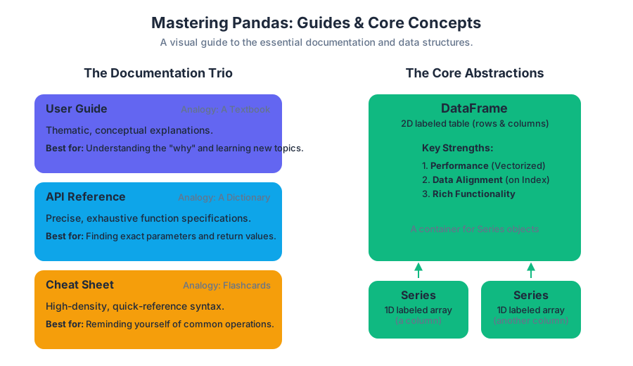
API Reference and Contribution Guide
Key concepts: Public vs. Private API · Contribution Workflow · Development Environment Setup · Code and Documentation Standards · Software Versioning · Release Notes
For advanced users and developers, this section covers the complete public API, the project's development lifecycle, and how to contribute to the pandas library. It also includes information on release notes to track the library's evolution.
API Reference and Contribution Guide
Transitioning from a proficient user of a library to a contributor or a power user who can build robust, long-lasting applications requires a deeper understanding of the project's structure, its development philosophy, and its public-facing contract. This guide serves as the bridge, providing a definitive overview of the library's Application Programming Interface (API), the complete workflow for contributing code and documentation, and the standards that ensure the project's quality and longevity. Mastering this material is essential for anyone looking to write mission-critical code that depends on this library or to participate directly in its evolution.
AI_SVGI_SVG## The API: A Contract with the User
At its core, a library's API is a formal contract. It defines the stable, predictable ways a user can interact with the software. However, not all functions, classes, and modules you can import are part of this contract. Understanding the distinction between the public and private API is the single most important concept for building reliable software that won't break when the library is updated.
Public vs. Private API
Public API: The set of classes, methods, functions, and parameters that the library developers have committed to supporting. The public API is stable; it will only change in predictable ways, typically with ample warning (deprecation periods) and clear documentation in release notes. Changes that break backward compatibility are reserved for major version releases.
Private API: The internal implementation details of the library. These are the functions, modules, and objects the library uses to do its work. They are not intended for external use and can be changed, renamed, or removed at any time, even in a minor patch release, without any warning.
Why This Distinction Matters
The separation of public and private APIs is fundamental to software engineering. It allows library developers the freedom to refactor, optimize, and improve the internal codebase without the fear of breaking user applications. For the user, it provides a stable foundation to build upon. Relying on the public API ensures that your code will continue to work across future versions of thelibrary (excluding major, breaking changes). Conversely, building an application that depends on private, internal components is brittle and almost guaranteed to fail unexpectedly during a routine dependency upgrade.
Identifying Public vs. Private APIs in Practice
In the Python ecosystem, and specifically within libraries like pandas, several conventions signal the status of an API component:
| Convention | Example | Status | Description |
|---|---|---|---|
| No Underscore Prefix | pandas.read_csv() |
Public | The primary, documented way to access functionality. |
| Single Underscore Prefix | _internal_method() |
Private | A strong convention indicating the method is for internal use only. |
| Dunder Methods | __len__() |
Public Protocol | Part of a public protocol (e.g., the container protocol), but should be used via public functions like len(df) rather than direct calls. |
| Underscore-Prefixed Modules | pandas.io.formats._css |
Private | The entire module is considered internal and subject to change. |
| Explicit Documentation | "This function is for internal use." | Private | The documentation will explicitly state the component is not part of the public API. |
Concrete Example: The Wrong and Right Way
Imagine you want to get the internal array manager for a pandas DataFrame. You might discover an internal attribute that seems to do the trick.
import pandas as pd
import numpy as np

# Create a sample DataFrame
df = pd.DataFrame(np.random.rand(3, 2), columns=['A', 'B'])

# --------------------------------------------------------------------
# INCORRECT: Relying on a private API
# The `_mgr` attribute is an internal implementation detail.
# This code could break in any future pandas release without warning.
# --------------------------------------------------------------------
try:
    # This is brittle and not guaranteed to exist or have the same structure
    internal_manager = df._mgr
    print(f"Accessed private attribute `_mgr`: {type(internal_manager)}")
except AttributeError:
    print("`_mgr` attribute does not exist in this version.")

# --------------------------------------------------------------------
# CORRECT: Using the public API
# The `.values` attribute and `.to_numpy()` method are documented,
# public ways to get a NumPy representation of the DataFrame's data.
# --------------------------------------------------------------------
numpy_array_values = df.values
numpy_array_method = df.to_numpy()

print(f"\nAccessed public attribute `.values`: {type(numpy_array_values)}")
print(f"Accessed public method `.to_numpy()`: {type(numpy_array_method)}")
The first approach is a ticking time bomb. The second approach is robust and guaranteed to work according to the library's versioning policy.
The Contribution Workflow: From Idea to Integration
Contributing to a large open-source project follows a structured, collaborative process designed to maintain code quality, ensure consistency, and incorporate changes smoothly. This workflow, largely managed through Git and platforms like GitHub, can be broken down into a sequence of distinct steps.
Step 1: Finding and Claiming an Issue
All work begins at the project's issue tracker. This is the central hub for bug reports, feature requests, and discussions about potential changes.
- For new contributors: Look for issues tagged with labels like
good first issueorhelp wanted. These are specifically curated to be accessible to newcomers. - Claiming an issue: Before you start writing code, leave a comment on the issue thread expressing your intent to work on it. This prevents duplicated effort and allows maintainers to provide early guidance.
Step 2: Forking, Branching, and Syncing
The project's main repository is not modified directly. Instead, contributors work on their own copy (a fork) and submit changes via a Pull Request.
Fork: A personal copy of a repository on your own GitHub account. Branch: An independent line of development within your fork. You should create a new, descriptively named branch for every issue you work on (e.g.,
fix/issue-12345orfeature/new-plotting-backend).
This model isolates your work, preventing your main branch from diverging from the original project's main branch. It's crucial to keep your fork's main branch synchronized with the original (often called upstream) repository.
Here is a typical command-line workflow for setting up your local environment and starting work on a new fix:
# 1. Clone your personal fork of the repository (replace with your username)
git clone git@github.com:your-username/pandas.git
cd pandas

# 2. Add the original repository as a remote named "upstream"
git remote add upstream https://github.com/pandas-dev/pandas.git

# 3. Fetch the latest changes from the upstream repository
git fetch upstream

# 4. Ensure your local main branch is up-to-date with the upstream main
git checkout main
git rebase upstream/main

# 5. Create a new branch for your work, based on the latest upstream main
#    Replace '12345-fix-datetime-parsing' with a descriptive name for your issue
git checkout -b 12345-fix-datetime-parsing upstream/main

# Now you are ready to start making changes on your new branch.
echo "Development environment ready on branch: $(git rev-parse --abbrev-ref HEAD)"
Step 3: The Development Loop: Code, Test, Document
A contribution is more than just code. It is a triad of implementation, validation, and explanation.
- Code: Implement the fix or feature. Adhere to the project's coding standards.
- Test: Write new tests that prove your code works correctly. For a bug fix, the ideal test is a regression test—one that fails before your change and passes after. This ensures the bug never reappears.
- Document: Update the documentation. If you've added a new function, it needs a complete docstring. If you've changed behavior, the relevant parts of the user guide or API reference must be updated.
Step 4: Submitting a Pull Request (PR)
Once your changes are complete and tested locally, you push your branch to your fork on GitHub and open a Pull Request. The PR is a formal proposal to merge your changes into the main project repository.
A high-quality PR description includes:
- A link to the issue it resolves (e.g., "Closes #12345").
- A clear explanation of what was changed and why.
- A summary of the approach taken.
- Confirmation that tests and documentation have been added.
Upon submission, automated checks (Continuous Integration, or CI) will run, testing your code on different operating systems and Python versions. All checks must pass.
Step 5: Code Review and Merging
After the PR is submitted, project maintainers and other community members will review your code. They may suggest improvements, ask for clarifications, or request changes. This is a collaborative process. Respond to feedback by pushing new commits to your branch; the PR will update automatically.
Once the reviewers are satisfied and all CI checks are green, a core maintainer will merge your Pull Request. Your contribution is now a part of the project!
Setting Up a Robust Development Environment
To effectively contribute, you must be able to build and test the library from source on your local machine.
Core Dependencies and Environment Management
A dedicated development environment is critical to avoid conflicts with other projects or your system's Python installation. Tools like conda or venv are standard.
| Tool | Purpose |
|---|---|
| Git | Version control system for managing code changes. |
| Python | The specific version(s) the project supports (e.g., Python 3.9+). |
| C/C++ Compiler | Required for building compiled extensions (e.g., Cython .pyx files). |
| Conda / venv | For creating isolated Python environments. |
| pip | For installing Python dependencies. |
Here is a shell script demonstrating how to set up a conda environment and install the necessary dependencies from the project's configuration files.
# Create a new conda environment named 'pandas-dev' with a specific Python version
conda create -n pandas-dev python=3.10 --yes

# Activate the newly created environment
conda activate pandas-dev

# Install dependencies using Mamba for speed (a faster conda alternative)
conda install -c conda-forge mamba --yes

# Install build, test, and documentation dependencies from environment files
# The `-c conda-forge` channel is often necessary for scientific packages
mamba install --file environment-dev.yml --file environment-test.yml -c conda-forge --yes

# Now, build the project's C/Cython extensions in-place
# The `-j 4` flag uses 4 parallel jobs to speed up compilation
python setup.py build_ext --inplace -j 4

echo "Build complete. You can now run the test suite."
Running the Test Suite
Before submitting a PR, you must run the test suite locally to catch any regressions. The pytest framework is commonly used.
- Run the full suite:
pytest pandas(This can take a long time). - Run tests for a specific module:
pytest pandas/tests/io/test_parsers.py - Run a specific test:
pytest pandas/tests/io/test_parsers.py -k "test_read_csv_with_quotes"
Upholding Project Standards
Large open-source projects thrive on consistency. Adhering to established standards for code, tests, and documentation makes the codebase more readable, maintainable, and easier for everyone to contribute to.
Code Style and Linting
Projects enforce a consistent code style to ensure readability. This is typically based on PEP 8, the official style guide for Python code. Automated tools called linters check the code for style violations.
| Tool | Purpose |
|---|---|
black |
An opinionated code formatter that automatically reformats code to a consistent style. |
flake8 |
A linter that checks for PEP 8 compliance, logical errors, and code complexity. |
isort |
A tool that automatically sorts imports alphabetically and groups them. |
These tools are often configured in a pyproject.toml file at the root of the repository.
# Example configuration in pyproject.toml for linting tools

[tool.black]
line-length = 88
target-version = ['py38', 'py39', 'py310']

[tool.isort]
profile = "black"
multi_line_output = 3

[tool.flake8]
# Ignore certain errors, e.g., E203 (whitespace before ':') which conflicts with black
ignore = "E203,W503"
max-line-length = 88
max-complexity = 18
Testing Philosophy and Implementation
A comprehensive test suite is the bedrock of a stable library. Every new feature must be accompanied by tests, and every bug fix must include a regression test.
Here is an example of a well-structured pytest regression test for a hypothetical bug where pd.to_datetime incorrectly parses a specific date format when a timezone is provided.
import pandas as pd
import pytest
from pandas.errors import ParserError

# A regression test for a hypothetical issue (e.g., GH#98765)

# Use a pytest marker to categorize the test
@pytest.mark.parametrize(
    "date_str, expected_tz",
    [
        ("2023-10-26T12:00:00Z", "UTC"),
        ("2023-10-26T12:00:00+01:00", "UTC+01:00"),
    ],
)
def test_to_datetime_iso_format_with_tz(date_str, expected_tz):
    """
    Test that to_datetime correctly parses ISO 8601 strings with timezone info.
    This is a regression test for GH#98765.
    """
    # The action: call the function being tested
    result = pd.to_datetime(date_str)

    # The validation: check that the output is correct
    assert result.year == 2023
    assert result.month == 10
    assert result.day == 26
    assert str(result.tz) == expected_tz

def test_to_datetime_invalid_format_raises():
    """
    Test that an invalid format correctly raises a specific error.
    """
    # Use pytest.raises to assert that a specific exception is thrown
    with pytest.raises(ParserError, match="Unknown string format"):
        pd.to_datetime("This is not a date")
Documentation Standards
Clear, comprehensive documentation is as important as the code itself. Docstrings within the code are the source of truth for the API reference. Most scientific Python projects, including pandas, use the numpydoc format.
A complete docstring includes several sections:
| Section | Content |
|---|---|
| Summary | A brief, one-line summary of the object's purpose. |
| Extended Summary | A more detailed explanation of what the object does. |
| Parameters | A description of each parameter, its type, and what it does. |
| Returns | A description of the returned object(s) and their types. |
| See Also | Links to related functions or methods. |
| Examples | One or more runnable examples demonstrating usage. |
Here is an example of a function with a complete numpydoc docstring:
def compute_weighted_average(values, weights):
    """
    Compute the weighted average of a sequence of values.

    This function calculates the weighted average, where each value is
    multiplied by its corresponding weight, summed, and then divided by
    the sum of the weights.

    Parameters
    ----------
    values : array-like
        A sequence of numbers to be averaged.
    weights : array-like
        A sequence of weights corresponding to each value. Must be the
        same length as `values`.

    Returns
    -------
    float
        The computed weighted average. Returns NaN if the sum of weights is zero.

    See Also
    --------
    numpy.average : A more feature-rich version of a weighted average.

    Examples
    --------
    >>> values = [10, 20, 30]
    >>> weights = [1, 2, 1]
    >>> compute_weighted_average(values, weights)
    20.0
    """
    import numpy as np
    values = np.asarray(values)
    weights = np.asarray(weights)

    if values.shape != weights.shape:
        raise ValueError("`values` and `weights` must have the same shape.")

    sum_of_weights = np.sum(weights)
    if sum_of_weights == 0:
        return np.nan

    return np.sum(values * weights) / sum_of_weights
Software Versioning and Release Cycle
Understanding how the software is versioned and released helps you manage dependencies and anticipate changes.
Semantic Versioning (SemVer)
Most open-source projects follow a versioning scheme called Semantic Versioning (SemVer). A version number is expressed as MAJOR.MINOR.PATCH.
Semantic Versioning (SemVer): Given a version number
MAJOR.MINOR.PATCH, increment the:
MAJORversion when you make incompatible API changes.MINORversion when you add functionality in a backward-compatible manner.PATCHversion when you make backward-compatible bug fixes.
This scheme provides clear expectations:
- Updating from
2.1.4to2.1.5(a patch release) should be safe; it only contains bug fixes. - Updating from
2.1.4to2.2.0(a minor release) adds new features but should not break your existing code. - Updating from
2.1.4to3.0.0(a major release) is a significant change that will likely require you to modify your code to adapt to breaking API changes.
The Deprecation Cycle
To avoid abrupt changes in major releases, libraries use a deprecation cycle. When a feature is scheduled for removal, it is first marked as deprecated.
- Warning: Using the feature will raise a
FutureWarningorDeprecationWarning, advising users to switch to a new alternative. - Grace Period: The feature remains functional for one or more minor releases, giving users time to update their code.
- Removal: In a future major release, the deprecated feature is removed entirely.
Understanding Release Notes
The Release Notes (or changelog) are the human-readable summary of all changes in a new version. They are an essential resource for anyone upgrading the library.
Structure and Content
Release notes are typically organized into categories to make them easy to parse:
- Enhancements: New features and additions.
- Bug Fixes: A list of bugs that were fixed, often with links to the original issue reports.
- API Changes: A critical section detailing any changes to the public API, including breaking changes.
- Deprecations: A list of all functions, methods, or parameters that are now deprecated.
- Performance Improvements: Notes on any significant optimizations.
Here is an example of what a release note entry might look like:
### Enhancements

* **New `DataFrame.explode()` method for list-like columns**

  The new `DataFrame.explode()` method transforms each element of a list-like to a row, replicating the index values. This is useful for un-nesting data. (GH#12345)

  **Old way:**
  ```python
  # Manual, more complex logic
New way:
df = pd.DataFrame({'A': [[1, 2], [3]], 'B': [1, 2]})
df.explode('A')
Reading the release notes *before* upgrading is a best practice. Pay special attention to the "API Changes" and "Deprecations" sections to understand what, if anything, in your code needs to be updated.
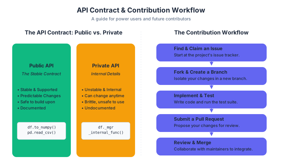
Community Tutorials and Next Steps
Key concepts: Beginner-friendly tutorials · Real-world data examples · Diverse learning formats (cookbooks, workshops, videos)
A collection of tutorials, workshops, and articles created by the pandas community. These resources are aimed at new users and often use real-world datasets to demonstrate fundamental and advanced concepts in diverse formats.
Community Tutorials and Next Steps
The official pandas documentation provides a robust and comprehensive foundation for learning the library's API. It is the canonical source for syntax, parameters, and core functionality. However, mastering pandas—or any powerful tool—involves more than just memorizing function signatures. It requires developing an intuition for problem-solving, understanding idiomatic patterns, and learning to navigate the complexities of real-world, messy data. This is where the vibrant ecosystem of community-created tutorials, workshops, and articles becomes an indispensable resource for the aspiring data practitioner.
This section serves as a curated portal to that ecosystem. It moves beyond the "what" of the API to the "how" and "why" of its application. These resources, built by fellow users and experts, offer diverse perspectives, practical examples, and domain-specific insights that bridge the gap between theoretical knowledge and practical mastery. They demonstrate not just how to use a function, but how to think with data.
AI_SVGI_SVG## The Learning Trajectory: From Fundamentals to Mastery
The journey to pandas proficiency can be conceptualized as a series of stages, each building upon the last. Community resources are particularly valuable for accelerating the transition between these stages, providing context and motivation that documentation alone often cannot.
Stage 1: Foundational Fluency (The "What" and "How")
This initial stage is about building a core vocabulary and understanding the fundamental objects. The goal is to become comfortable with the basic mechanics of data manipulation.
Core Concepts:
- Data Structures: The
DataFrameas a 2D table and theSeriesas its 1D column counterpart.- I/O: Reading data from common formats like CSV (
pd.read_csv) and writing to formats like Excel (.to_excel).- Inspection: Basic examination of a
DataFrameusing.head(),.tail(),.info(), and.describe().- Selection: Subsetting data using column selection (
df['col']), conditional filtering (boolean indexing), and the primary accessors: label-based.locand integer-position-based.iloc.- Creation: Deriving new columns from existing ones through vectorized arithmetic operations.
At this stage, learning is focused on direct, single-step operations. Community tutorials often excel here by providing compelling, real-world datasets (like the Titanic or air quality data mentioned in the official guides) that make these initial steps more engaging than working with abstract, manually created tables.
Stage 2: Analytical Dexterity (The "Why")
Once the fundamentals are in place, the focus shifts to combining these building blocks to answer complex analytical questions. This is the heart of data analysis, where raw data is transformed into insight.
Core Concepts:
- Aggregation: Calculating summary statistics (
.mean(),.sum(),.count()) across an entire dataset or specific columns.- Grouping: The split-apply-combine pattern, implemented via the
.groupby()method, is arguably the most powerful concept in pandas. It allows for calculating statistics on a per-category basis.- Reshaping: Transforming the layout of data. This includes pivoting from a long format to a wide format (
.pivot()or.pivot_table()) and un-pivoting from wide to long (.melt()).- Combining: Merging and concatenating multiple
DataFrameobjects. This involvespd.concat()for stacking data andpd.merge()for database-style joins.
This stage is less about learning new functions in isolation and more about composing them into analytical pipelines. Community "cookbooks" and project-based tutorials are invaluable here, as they frame these operations within the context of a larger analytical goal.
Stage 3: Specialized Applications (The "What If")
With a solid grasp of general data manipulation, practitioners often need to develop expertise in specific domains. pandas has rich, specialized toolsets for common data types that go far beyond basic operations.
Core Concepts:
- Time Series: Handling date and time data, including parsing strings to datetime objects (
pd.to_datetime), using the.dtaccessor to extract components (year, month, weekday), and resampling data to different frequencies (.resample()).- Text Processing: Manipulating string data using the
.straccessor, which provides vectorized access to Python's string methods like.lower(),.contains(),.split(), and.replace().- Categorical Data: Using the
categorydata type for columns with a fixed, limited number of unique values to save memory and improve performance.
Workshops and deep-dive articles from the community are critical for this stage. They often focus on a single domain, such as financial time series analysis or natural language processing (NLP) preprocessing, showcasing advanced techniques and idiomatic patterns that are not immediately obvious from the API reference.
A Curated Guide to Community Resources
The landscape of community content is vast. Understanding the different formats and their strengths can help you choose the right resource for your learning goals.
Interactive Cookbooks: Problem-Oriented Learning
A cookbook is a collection of "recipes," where each recipe provides a step-by-step solution to a specific, practical problem. This format is highly effective for moving from Stage 1 to Stage 2, as it directly connects code to a tangible outcome.
- What It Is: A goal-oriented guide, often structured as a series of questions (e.g., "How do I find the top 3 items per category?"). Julia Evans's pandas cookbook is a classic example of this style.
- Why It Matters: Cookbooks teach patterns, not just functions. They help you recognize recurring analytical problems and map them to idiomatic pandas solutions. They are excellent for building a mental library of reusable code snippets.
- Concrete Example: A common and non-trivial task is to select the top N rows within each group defined by a categorical column. For example, finding the three most expensive products in each product category.
This problem requires a combination of .groupby() and a selection method. Here is a robust, real-world implementation in Python.
import pandas as pd
import numpy as np

# Create a realistic, non-trivial DataFrame
np.random.seed(42)
num_rows = 1000
data = {
    'category': np.random.choice(['Electronics', 'Apparel', 'Home Goods', 'Groceries'], num_rows),
    'product_id': [f'P{i:04d}' for i in range(num_rows)],
    'price': np.round(np.random.lognormal(mean=3.5, sigma=1.0, size=num_rows), 2),
    'stock_level': np.random.randint(0, 200, size=num_rows)
}
products_df = pd.DataFrame(data)

# --- The "Recipe": Find the top 3 most expensive products per category ---

# Method 1: Using sort_values() and groupby().head()
# This is intuitive and often sufficient for moderately sized data.
top_3_expensive_v1 = (
    products_df
    .sort_values(by=['category', 'price'], ascending=[True, False])
    .groupby('category')
    .head(3)
)

# Method 2: Using groupby().nlargest()
# This can be more performant as it avoids a full sort of the entire DataFrame.
# It performs a selection within each group.
top_3_expensive_v2 = (
    products_df
    .groupby('category', group_keys=False)
    .apply(lambda x: x.nlargest(3, 'price'))
)

# Method 3: A more modern approach with .nlargest() on the grouped object directly
# This is often the most efficient and idiomatic way.
top_3_expensive_v3 = products_df.groupby('category')['price'].nlargest(3).reset_index()
# This returns the indices, so we need to merge back to get full data
top_products_df = pd.merge(
    top_3_expensive_v3,
    products_df.drop('price', axis=1),
    left_on=['category', 'level_1'],
    right_on=['category', products_df.index.name or 'index']
).drop(columns=['level_1'])

print("--- Top 3 Expensive Products (Method 1: sort_values) ---")
print(top_3_expensive_v1)
This single problem highlights a key aspect of pandas: there are often multiple ways to achieve the same result, with different trade-offs in readability and performance. A good cookbook recipe not only provides a solution but often compares alternatives. This same problem is a classic in the database world, where it is typically solved using window functions.
-- SQL equivalent for finding the top 3 most expensive products per category
-- This uses a Common Table Expression (CTE) and the ROW_NUMBER() window function.

WITH RankedProducts AS (
    SELECT
        category,
        product_id,
        price,
        stock_level,
        ROW_NUMBER() OVER(PARTITION BY category ORDER BY price DESC) as price_rank
    FROM
        products
)
SELECT
    category,
    product_id,
    price,
    stock_level
FROM
    RankedProducts
WHERE
    price_rank <= 3;
Comparing the pandas and SQL approaches reveals deep parallels in data manipulation logic, reinforcing the underlying concepts of partitioning, ordering, and filtering.
| Method Comparison for Top-N-per-Group | Readability | Performance | Key Idea |
|---|---|---|---|
sort_values().groupby().head(N) |
High | Good (can be slow on huge data due to full sort) | Sort everything first, then take the top from each group. |
groupby().apply(lambda x: x.nlargest(N)) |
Medium | Variable (Python lambda overhead) | Apply a selection function to each group sub-frame. |
groupby().nlargest(N) |
High | Excellent | Uses optimized internal C-level implementation for selection. |
SQL ROW_NUMBER() |
High (for SQL users) | Excellent (in a database engine) | Assign a rank within each partition, then filter on rank. |
Deep-Dive Workshops and Video Series: Guided Exploration
Workshops and video tutorials offer a narrative-driven learning experience. They guide the user through a complete project, from data acquisition to final analysis or visualization, showing the thought process, debugging steps, and decision-making along the way.
- What It Is: A structured, multi-part educational series, often led by an instructor. Examples include conference tutorials (from PyCon, SciPy) or online courses.
- Why It Matters: This format excels at teaching workflow and context. You don't just see the final, polished code; you see the iterative process of building it. This is crucial for understanding how pandas fits into a larger data science pipeline.
- Concrete Example: A common workshop theme is building an end-to-end data cleaning pipeline. This typically involves steps that occur before pandas is even imported. A shell script might be used to orchestrate the initial stages.
#!/bin/bash

# --- Data Acquisition and Preparation Script ---
# This script demonstrates the steps before data even enters a Python environment.

# Set variables
DATA_URL="https://raw.githubusercontent.com/datasciencedojo/datasets/master/titanic.csv"
RAW_DIR="data/raw"
PROCESSED_DIR="data/processed"
FILENAME="titanic.csv"
RAW_FILE_PATH="$RAW_DIR/$FILENAME"

echo "--- Setting up directories ---"
mkdir -p $RAW_DIR
mkdir -p $PROCESSED_DIR

echo "--- Downloading Titanic dataset from $DATA_URL ---"
# Use curl to download the data, -s for silent, -o for output file
curl -s -o $RAW_FILE_PATH $DATA_URL

# Basic validation and inspection in the shell
echo "--- Basic file inspection ---"
if [ -f "$RAW_FILE_PATH" ]; then
    echo "File downloaded successfully."
    echo "First 5 lines of the raw data:"
    head -n 5 $RAW_FILE_PATH
    echo "Number of lines in the file (including header):"
    wc -l < $RAW_FILE_PATH
else
    echo "ERROR: File download failed."
    exit 1
fi

echo "--- Running the pandas cleaning script ---"
# Now, invoke the Python script that will use pandas to clean the data
# We pass the input and output paths as arguments for a robust pipeline
python scripts/clean_titanic.py --input_path $RAW_FILE_PATH --output_path $PROCESSED_DIR/cleaned_titanic.parquet

echo "--- Pipeline finished. Cleaned data is in $PROCESSED_DIR ---"
This script shows that a data analysis project is more than just a Jupyter Notebook. It involves orchestration, file management, and clear separation of raw and processed data—all concepts that a good workshop will emphasize.
| Typical Data Cleaning Workshop Curriculum | Key pandas Functions | Learning Objective |
|---|---|---|
| Module 1: Ingestion & Inspection | pd.read_csv, .info(), .describe(), .dtypes |
Load data correctly and perform an initial diagnostic assessment. |
| Module 2: Handling Missing Data | .isna(), .sum(), .dropna(), .fillna() |
Identify, quantify, and implement strategies for missing values (imputation, deletion). |
| Module 3: Data Type Correction | .astype(), pd.to_datetime, pd.to_numeric |
Ensure all columns are represented by the correct and most efficient data type. |
| Module 4: Outlier & Error Correction | Boolean indexing, .clip(), .loc |
Detect and handle anomalous or invalid data points. |
| Module 5: Text & Categorical Cleanup | .str accessor, .replace(), .map() |
Standardize string data (e.g., trim whitespace, fix casing) and encode categoricals. |
AI_DEMOI_DEMO### Articles and Blog Posts: Specialized Knowledge
While cookbooks solve common problems and workshops teach workflows, articles and blog posts are where the community shares deep, specialized knowledge. These are often written by advanced practitioners who have encountered and solved a particularly tricky problem.
- What It Is: A focused, in-depth written piece on a specific topic, such as performance optimization, a subtle aspect of the API, or a comparison with another library.
- Why It Matters: This is the frontier of community knowledge. It's where you learn about performance bottlenecks, memory management, and how to push the boundaries of what's possible with the library.
- Concrete Example: A frequent topic of advanced articles is memory optimization. A default
pd.read_csvoften uses far more memory than necessary by assigning genericint64,float64, andobjectdtypes. An expert-level article would demonstrate how to significantly reduce aDataFrame's memory footprint.
Here is a before-and-after code block demonstrating these optimization techniques.
import pandas as pd
import numpy as np

# Create a large, unoptimized DataFrame to simulate real-world data
num_rows = 5_000_000
data = {
    'user_id': np.random.randint(1, 100_000, size=num_rows),
    'product_category': np.random.choice(['CatA', 'CatB', 'CatC', 'CatD', 'CatE'] * 20, size=num_rows),
    'rating': np.random.randint(1, 6, size=num_rows),
    'price': np.random.uniform(10.0, 1000.0, size=num_rows).round(2),
    'country_code': np.random.choice(['US', 'GB', 'DE', 'FR', 'CA', 'JP'], size=num_rows)
}
df_unoptimized = pd.DataFrame(data)

# --- BEFORE: Check memory usage of the unoptimized DataFrame ---
mem_before = df_unoptimized.memory_usage(deep=True).sum() / 1024**2  # in MiB
print(f"--- Unoptimized DataFrame ---")
print(df_unoptimized.info(memory_usage='deep'))
print(f"\nInitial memory usage: {mem_before:.2f} MiB")

# --- AFTER: Apply memory optimization techniques ---
df_optimized = df_unoptimized.copy()

# 1. Downcast integer columns
df_optimized['user_id'] = pd.to_numeric(df_optimized['user_id'], downcast='integer')
df_optimized['rating'] = pd.to_numeric(df_optimized['rating'], downcast='integer')

# 2. Downcast float columns
df_optimized['price'] = pd.to_numeric(df_optimized['price'], downcast='float')

# 3. Convert object columns with low cardinality to 'category'
for col in ['product_category', 'country_code']:
    if df_optimized[col].nunique() / len(df_optimized[col]) < 0.5:
        df_optimized[col] = df_optimized[col].astype('category')

mem_after = df_optimized.memory_usage(deep=True).sum() / 1024**2
print(f"\n--- Optimized DataFrame ---")
print(df_optimized.info(memory_usage='deep'))
print(f"\nOptimized memory usage: {mem_after:.2f} MiB")

# --- Report the results ---
reduction = (mem_before - mem_after) / mem_before * 100
print(f"\nMemory reduction: {reduction:.2f}%")
This practical example provides a powerful lesson: understanding data types is not just an academic exercise; it has a direct and massive impact on performance and resource consumption, especially when working with large datasets.
Data Type Comparison: object vs. category |
object (String) |
category |
|---|---|---|
| Memory Storage | Stores a full Python string for each element. High memory usage. | Stores integer "codes" and a single lookup table (the "categories"). Very low memory for low-cardinality data. |
| Performance | Group-by and merge operations are string-based, which is computationally slow. | Operations are performed on the integer codes, which is extremely fast. |
| Use Case | High-cardinality text data (e.g., user comments, unique IDs). | Low-cardinality text data (e.g., country codes, status flags, product categories). |
| Common Pitfall | The default dtype for non-numeric columns from read_csv. Can silently consume vast amounts of RAM. |
Can cause issues if new, unseen categories are introduced without being added to the category list first. |
By engaging with these community resources, you not only learn the syntax of pandas but also the craft of data analysis. You learn to write code that is not only correct but also efficient, readable, and idiomatic, preparing you for complex, real-world data challenges.
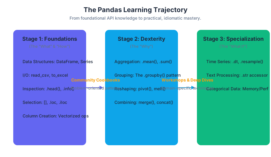
Source Materials
Study pandas documentation with AI — Free on Lykke
Sign up for free to generate personalized flashcards, quizzes, and study guides from this course. Chat with an AI tutor that knows the material.
Get Started FreeView this course wiki on Lykke · Browse all public course wikis