Numerical Analysis and Computational Methods

Introduction and Python for Numerical Computing

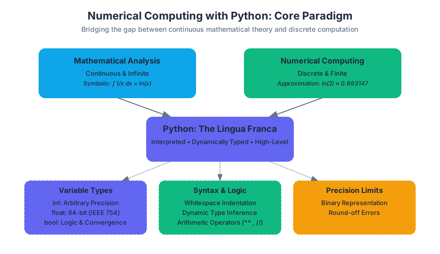
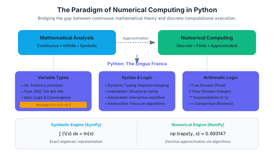
Numerical analysis is the study of algorithms that use numerical approximation for the problems of mathematical analysis. In the modern era, this discipline is inseparable from the computational tools used to implement it. While theoretical mathematics often deals with the infinite and the continuous, computers are finite and discrete. This fundamental tension—representing the continuous within the discrete—is the heart of numerical computing.

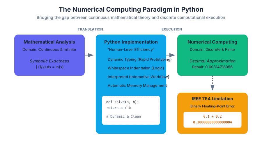
Python has emerged as the lingua franca of this field. Its rise is not due to raw execution speed, but rather its "human-level" efficiency: the speed with which a researcher can translate a complex mathematical model into a functioning program. This section explores the foundational syntax and logic of Python, specifically through the lens of numerical application.

The Paradigm of Numerical Computing

Numerical computing differs from symbolic computing. While a symbolic engine (like Mathematica or SymPy) might tell you that the integral of $1/x$ is $\ln(x)$, a numerical engine (like the ones we will build in Python) provides a decimal approximation, such as $0.693147$.

Definition: Numerical Analysis The branch of mathematics that designs and analyzes algorithms for obtaining numerical solutions to problems that involve continuous variables. These problems arise throughout the natural sciences, social sciences, engineering, medicine, and business.

In this course, we utilize Python because it abstracts away low-level memory management, allowing us to focus on the stability and convergence of our algorithms. However, this abstraction requires a deep understanding of how Python handles data types and operations to avoid "silent" errors in precision.

Python Syntax and the Interpreter Environment

Python is an interpreted, high-level, dynamically typed language. Unlike compiled languages such as C++ or Fortran, Python code is executed line-by-line by the Python Interpreter. This allows for an interactive workflow, which is essential when testing numerical convergence or visualizing data.

The Role of Indentation

In most programming languages, curly braces {} or keywords like begin/end define blocks of code. Python uses whitespace indentation. This is not merely a stylistic choice but a syntactic requirement.

# A simple example of Python's clean syntax
def calculate_area(radius):
    pi = 3.141592653589793
    area = pi * (radius ** 2)
    return area

print(calculate_area(5))

Implicit vs. Explicit Declaration

One of Python's most powerful features for rapid prototyping is dynamic typing. You do not need to declare that a variable is an integer or a float; the interpreter infers the type at runtime based on the value assigned.

Feature	Python Approach	Benefit for Numerical Work
Typing	Dynamic	Faster implementation of formulas
Memory	Automatic Garbage Collection	Focus on logic, not memory leaks
Syntax	Minimalist (No semicolons)	Reduces visual noise in complex equations
Libraries	Extensive (NumPy, SciPy)	Access to optimized C-level routines

Variable Types and Memory Representation

In numerical computing, the type of a variable dictates the precision of your result. Python handles several standard types, but for our purposes, int, float, and bool are the most critical.

Integers (int)

Python 3 integers have arbitrary precision. This means they can grow as large as your computer's memory allows, avoiding the "overflow" errors common in 32-bit or 64-bit integer types in other languages.

Floating-Point Numbers (float)

In Python, float corresponds to double-precision (64-bit) binary floating-point numbers, following the IEEE 754 standard.

Key Insight: The Floating-Point Limitation Because computers represent numbers in base-2 (binary), certain base-10 decimals cannot be represented exactly. For example, 0.1 + 0.2 in Python results in 0.30000000000000004. In numerical analysis, managing these "round-off errors" is a primary concern.

Booleans (bool)

Representing True or False, booleans are the backbone of conditional logic and convergence criteria (e.g., "Stop the loop when the error is less than $10^{-6}$").

Arithmetic Operators and Mathematical Logic

Python provides a robust set of operators to perform calculations. Understanding the distinction between different division types is particularly important for algorithm design.

Basic Arithmetic

The standard operators follow expected mathematical conventions:

• + (Addition)
• - (Subtraction)
• * (Multiplication)
• / (True Division): Always returns a float.
• // (Floor Division): Divides and rounds down to the nearest whole number.
• % (Modulo): Returns the remainder of the division.
• ** (Exponentiation): $x^y$ is written as x ** y.

Comparison and Logical Operators

These operators evaluate expressions to return a Boolean value, which is essential for implementing piecewise functions or iterative loops.

Operator	Description	Example
==	Equal to	5 == 5 (True)
!=	Not equal to	5 != 3 (True)
>	Greater than	5 > 10 (False)
<	Less than	2 < 4 (True)
and	Logical AND	True and False (False)
or	Logical OR	True or False (True)
not	Logical NOT	not True (False)

Worked Example: The Quadratic Formula

To see these operators in action, consider the calculation of the discriminant in the quadratic formula $D = b^2 - 4ac$:

# Coefficients for x^2 + 5x + 6 = 0
a = 1
b = 5
c = 6

# Calculating the discriminant
discriminant = b**2 - 4*a*c

# Using comparison logic
if discriminant > 0:
    root1 = (-b + discriminant**0.5) / (2*a)
    root2 = (-b - discriminant**0.5) / (2*a)
    print(f"Roots are real: {root1}, {root2}")
elif discriminant == 0:
    root = -b / (2*a)
    print(f"One real root: {root}")
else:
    print("Roots are complex")

Operator Precedence: The Hierarchy of Evaluation

In numerical computing, a single misplaced parenthesis can lead to catastrophic errors in simulation. Python follows a specific hierarchy, often summarized by the acronym PEMDAS (Parentheses, Exponents, Multiplication/Division, Addition/Subtraction).

The Precedence Table

The following table ranks operators from highest precedence (evaluated first) to lowest (evaluated last).

Rank	Operator	Description
1	()	Parentheses (Grouping)
2	**	Exponentiation
3	+x, -x, ~x	Unary plus, minus, bitwise NOT
4	*, /, //, %	Multiplication, Division, Floor Div, Modulo
5	+, -	Addition, Subtraction
6	<<, >>	Bitwise shifts
7	&	Bitwise AND
8	^	Bitwise XOR
9	|	Bitwise OR
10	==, !=, >, <, etc.	Comparisons
11	not	Logical NOT
12	and	Logical AND
13	or	Logical OR

Case Study: Evaluating Complex Expressions

Consider the expression for a Gaussian distribution: $$f(x) = \frac{1}{\sigma\sqrt{2\pi}} e^{-\frac{1}{2}(\frac{x-\mu}{\sigma})^2}$$

In Python, without proper attention to precedence, this could be written incorrectly. Let's break down the correct implementation:

import math

x = 1.0
mu = 0.0
sigma = 1.0

# Correct implementation using precedence and parentheses
fx = (1 / (sigma * math.sqrt(2 * math.pi))) * math.exp(-0.5 * ((x - mu) / sigma)**2)

Common Pitfall: Writing 1 / sigma * math.sqrt(...) would result in $(1/\sigma) \cdot \sqrt{\dots}$ instead of $1 / (\sigma \cdot \sqrt{\dots})$. Always use parentheses to make the denominator explicit.

Computational Applications: Why We Compute

Numerical computing is not an abstract exercise; it is the engine of modern engineering. When analytical (exact) solutions are impossible to find, we turn to numerical approximations.

1. Space Exploration and Orbital Mechanics

Calculating the trajectory of a spacecraft requires solving systems of differential equations that have no closed-form solution. By discretizing time into small steps ($\Delta t$), we can use Python to predict the position of a rover on Mars with millimeter precision.

2. Autonomous Vehicles

Self-driving cars process LIDAR and camera data in real-time. This involves massive matrix multiplications and optimization algorithms (like Gradient Descent) implemented using the very operators discussed above. The speed and accuracy of these numerical calculations are literally a matter of life and death.

3. Financial Modeling

The Black-Scholes model for option pricing or Monte Carlo simulations for risk assessment rely on generating millions of random numerical outcomes to find an expected value.

Application	Numerical Method Used	Role of Python
Weather Prediction	Fluid Dynamics Simulations	Handling large multi-dimensional arrays
Structural Engineering	Finite Element Analysis (FEA)	Solving massive systems of linear equations
Machine Learning	Backpropagation / Optimization	Efficiently updating weights via partial derivatives

Common Pitfalls in Numerical Python

As you begin implementing algorithms, be wary of these common "gotchas" that can derail your computations.

1. Integer Division in Older Versions: In Python 2, 5/2 resulted in 2. In Python 3, it correctly results in 2.5. However, if you specifically need an integer, you must use 5 // 2.
2. Floating Point Equality: Never use == to compare two floats. Because of round-off errors, 0.1 + 0.2 == 0.3 will return False. Instead, check if the difference is smaller than a tiny tolerance (epsilon): abs(a - b) < 1e-9.
3. Mutable Default Arguments: While not strictly numerical, assigning a list as a default argument in a function can lead to shared state across function calls, corrupting numerical data.
4. Shadowing Built-in Names: Avoid naming your variables sum, min, max, or type, as these are built-in Python functions. Doing so will "shadow" the function, making it inaccessible later in your script.

Summary of the Computational Pipeline

The journey from a mathematical concept to a numerical result follows a structured pipeline.

1. Mathematical Modeling: Define the continuous equations (e.g., Newton's Laws).
2. Discretization: Convert the continuous model into a discrete form suitable for a computer.
3. Algorithm Design: Choose a method (e.g., Euler's method, Newton-Raphson).
4. Implementation: Write the Python code using correct variables, operators, and precedence.
5. Verification: Test against known solutions and check for numerical stability.

By mastering the basic syntax and understanding the underlying logic of Python's arithmetic, you lay the groundwork for the more complex iterative methods that define numerical analysis.

Mathematical Foundations and Error Analysis

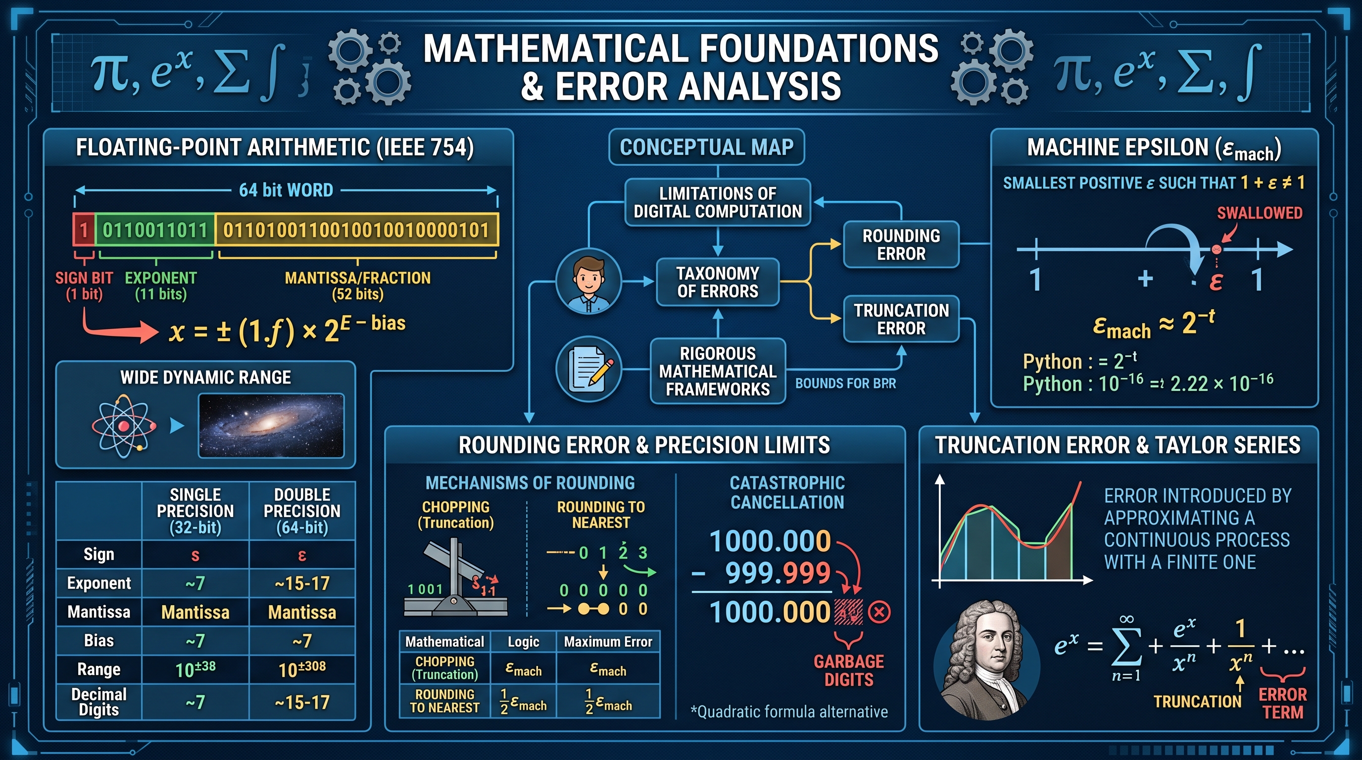
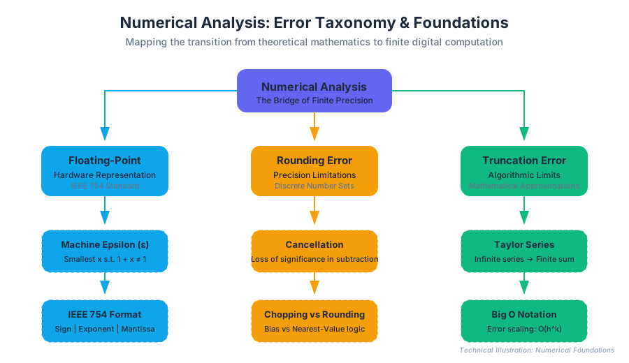
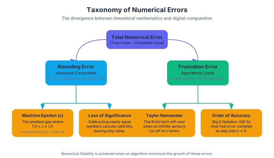
Numerical analysis is the bridge between the infinite precision of theoretical mathematics and the finite constraints of physical hardware. While a mathematician might comfortably work with the transcendental number $\pi$ or the infinite series for $e^x$, a computer scientist must grapple with the reality that a CPU can only represent a sliver of the real number line. This section explores the fundamental limitations of digital computation, the taxonomy of errors that arise during calculation, and the rigorous mathematical frameworks used to bound these errors.

Floating-Point Arithmetic

At the core of modern computing lies the Floating-Point Representation. Unlike fixed-point arithmetic, which allocates a set number of digits for the integer and fractional parts, floating-point arithmetic allows the "point" to move, providing a wide dynamic range that can represent both the diameter of an atom and the distance to a distant galaxy using the same number of bits.

The IEEE 754 Standard

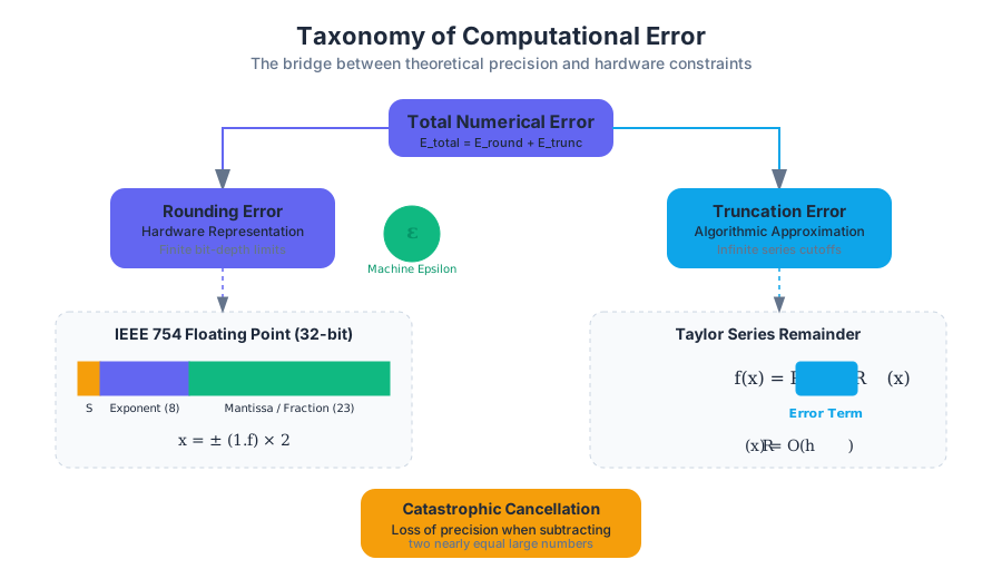
Most modern systems adhere to the IEEE 754 standard, which defines how floating-point numbers are stored in binary. A number $x$ is typically represented in the form:

Definition: Floating-Point Normalized Form $$x = \pm (1.f) \times 2^{E - bias}$$ Where:

• $s$ (Sign bit): Determines if the number is positive (0) or negative (1).
• $f$ (Fraction/Mantissa): The fractional part of the significand. The "1." is implicit in normalized numbers to save a bit.
• $E$ (Exponent): An unsigned integer that is shifted by a bias to allow for negative exponents.

Feature	Single Precision (32-bit)	Double Precision (64-bit)
Sign Bit	1 bit	1 bit
Exponent	8 bits	11 bits
Mantissa	23 bits	52 bits
Bias	127	1023
Approx. Range	$10^{-38}$ to $10^{38}$	$10^{-308}$ to $10^{308}$
Decimal Digits	~7	~15-17

Machine Epsilon ($\epsilon_{mach}$)

The most critical constant in numerical analysis is Machine Epsilon. It represents the upper bound on the relative error due to rounding in floating-point arithmetic.

Theorem: Machine Epsilon Machine epsilon is the smallest positive number $\epsilon$ such that $1 + \epsilon \neq 1$ in the computer's floating-point representation. For a system with $t$ bits in the mantissa, $\epsilon_{mach} \approx 2^{-t}$.

In Python, which uses double precision (64-bit) by default for floats, $\epsilon_{mach}$ is approximately $2.22 \times 10^{-16}$. This means that any calculation involving numbers of vastly different scales (e.g., adding $10^{16}$ and $1$) will result in the smaller number being "swallowed" by the larger one.

# Demonstrating Machine Epsilon in Python
x = 1.0
epsilon = 1.0
while 1.0 + epsilon != 1.0:
    last_epsilon = epsilon
    epsilon /= 2.0

print(f"Calculated Machine Epsilon: {last_epsilon}")
# Output: 2.220446049250313e-16

Rounding Error and Precision Limits

Rounding Error occurs because the set of representable floating-point numbers is discrete and finite. When a real number $x$ cannot be represented exactly, the system must choose a nearby representable number $fl(x)$.

Mechanisms of Rounding

There are two primary ways a system handles numbers it cannot represent exactly:

1. Chopping (Truncation): Simply discarding all bits beyond the available precision. This is computationally cheap but introduces a significant bias.
2. Rounding to Nearest: Choosing the representable value closest to the true value. This is the default behavior for IEEE 754.

Method	Mathematical Logic	Maximum Error
Chopping	$fl(x) = x$ truncated	$\epsilon_{mach}$
Rounding	$fl(x) = \text{nearest } \hat{x}$	$\frac{1}{2}\epsilon_{mach}$

Catastrophic Cancellation

One of the most dangerous forms of rounding error is Loss of Significance, often called Catastrophic Cancellation. This occurs when subtracting two nearly equal numbers. Because the leading digits of both numbers match, they cancel out, leaving only the "garbage" digits (the rounding errors) in the result.

Worked Example: Quadratic Formula Consider solving $ax^2 + bx + c = 0$ where $b^2 \gg 4ac$. If $b = 1000.000$ and $4ac = 0.0001$, then $\sqrt{b^2 - 4ac}$ is very close to $b$. Subtracting $-b + \sqrt{b^2 - 4ac}$ will lead to a massive loss of precision. Numerical software often uses an alternative form: $$x_1 = \frac{-2c}{b + \sqrt{b^2 - 4ac}}$$ to avoid this subtraction.

Truncation Error and Taylor Series

While rounding error is a byproduct of hardware, Truncation Error is a byproduct of the algorithm. It is the error introduced by approximating a continuous mathematical process with a finite one.

The Taylor Series Foundation

Most numerical methods (differentiation, integration, root-finding) are derived from the Taylor Series Expansion.

Taylor's Theorem If a function $f(x)$ is $n+1$ times continuously differentiable on an interval containing $a$, then for any $x$ in the interval: $$f(x) = \sum_{k=0}^{n} \frac{f^{(k)}(a)}{k!}(x-a)^k + R_n(x)$$ where $R_n(x)$ is the Remainder Term (the truncation error): $$R_n(x) = \frac{f^{(n+1)}(\xi)}{(n+1)!}(x-a)^{n+1}$$ for some $\xi$ between $a$ and $x$.

Big O Notation and Convergence

We quantify truncation error using Big O Notation, which describes how the error scales as the step size $h$ (where $h = x - a$) approaches zero.

• If $Error \approx Ch^k$, we say the method is $k$-th order accurate, written as $O(h^k)$.
• A higher order means the error drops much faster as we increase the resolution (decrease $h$).

Method	Order	Error Scaling
Forward Difference	$O(h)$	Halving $h$ halves error
Central Difference	$O(h^2)$	Halving $h$ quarters error
Simpson's Rule	$O(h^4)$	Halving $h$ reduces error by $1/16$

import math

def taylor_exp(x, n):
    """Approximate e^x using n terms of Taylor series."""
    approximation = sum([(x**i) / math.factorial(i) for i in range(n)])
    return approximation

true_val = math.exp(1.0)
approx_val = taylor_exp(1.0, 5)
truncation_error = abs(true_val - approx_val)

print(f"True e: {true_val}")
print(f"Approx (5 terms): {approx_val}")
print(f"Truncation Error: {truncation_error}")

Absolute vs. Relative Error

To discuss error meaningfully, we must distinguish between the magnitude of the mistake and its significance relative to the scale of the problem.

Definitions

Let $x$ be the true value and $\hat{x}$ be the approximation.

1. Absolute Error ($E_{abs}$): $$E_{abs} = |x - \hat{x}|$$ Use case: When the physical units of the error matter (e.g., "the bridge is off by 2 centimeters").

2. Relative Error ($E_{rel}$): $$E_{rel} = \frac{|x - \hat{x}|}{|x|}, \quad x \neq 0$$ Use case: When the scale of the value matters. An error of 1 meter is catastrophic when measuring a room, but negligible when measuring the distance to the moon.

Comparison Table

Scenario	True Value ($x$)	Approx ($\hat{x}$)	Abs Error	Rel Error
Small Scale	0.001	0.0009	0.0001	10%
Large Scale	1,000,000	999,999	1.0	0.0001%
Precision Limit	$\pi$	3.14159	$2.65 \times 10^{-6}$	$8.4 \times 10^{-7}$

Insight: Significant Digits A common rule of thumb is that if the relative error is approximately $10^{-d}$, the approximation $\hat{x}$ has roughly $d$ correct significant decimal digits.

Stability and Error Propagation

Numerical analysis is rarely a single step. It is usually a pipeline where the output of one function becomes the input of the next. Error Propagation is the study of how errors grow or shrink through these steps.

Forward vs. Backward Error

• Forward Error: The difference between the calculated result and the true result ($|f(x) - \hat{f}(x)|$).
• Backward Error: The smallest change to the input $x$ that would make the calculated result "correct" for that modified input ($|x - \hat{x}|$ such that $\hat{f}(x) = f(\hat{x})$).

Condition Numbers

The Condition Number ($\kappa$) of a function measures how sensitive the output is to small changes in the input.

$$ \kappa = \left| \frac{x f'(x)}{f(x)} \right| $$

• Well-conditioned: $\kappa$ is small (near 1). Small changes in input lead to small changes in output.
• Ill-conditioned: $\kappa$ is large. Small input errors (like rounding) are magnified into massive output errors.

Condition Number ($\kappa$)	Interpretation
$\kappa \approx 1$	Stable; error does not grow.
$\kappa \approx 10^k$	You may lose $k$ digits of precision.
$\kappa \to \infty$	Singular problem; unsolvable numerically.

Stability of Algorithms

An algorithm is Stable if the errors generated during the calculation do not grow uncontrollably. A classic example is the evaluation of a polynomial. Using the standard form $a_n x^n + \dots + a_0$ can be unstable for high degrees, whereas Horner’s Method reduces the number of multiplications and additions, leading to better numerical stability.

def horner_eval(coeffs, x):
    """
    Evaluates a polynomial using Horner's Method.
    coeffs: [a_n, a_{n-1}, ..., a_0]
    """
    result = 0
    for c in coeffs:
        result = result * x + c
    return result

# Evaluating P(x) = 3x^2 + 2x + 1 at x=2
# Standard: 3*(2^2) + 2*(2) + 1 = 12 + 4 + 1 = 17
# Horner: ((3*2) + 2)*2 + 1 = (8)*2 + 1 = 17

Common Pitfalls in Numerical Computing

1. Testing for Equality: Never use if x == 0.3: when dealing with floats. Instead, use a tolerance: if abs(x - 0.3) < 1e-9:.
2. Summing Series: When summing a long list of numbers, sum from smallest to largest. Adding a tiny number to a large running sum results in the tiny number being rounded away.
3. Overflow and Underflow:
   • Overflow: The result is too large to be represented (becomes inf).
   • Underflow: The result is too small (closer to zero than the smallest representable normalized number), often resulting in it being flushed to 0.0.
4. The "Hidden" Truncation: Using a library function (like sin(x)) assumes you trust its internal Taylor expansion or CORDIC algorithm. Always check the documentation for the precision guarantees of third-party libraries.

Summary of Error Sources

Error Source	Origin	Mitigation Strategy
Modeling Error	Simplifications in the physics/math	Use more complex models.
Data Error	Measurement noise in inputs	Use statistical filtering/smoothing.
Rounding Error	Finite bit representation	Use higher precision (Double/Quad).
Truncation Error	Finite approximation of infinite series	Increase number of terms or decrease step size.
Propagation Error	Sensitivity of the algorithm	Use well-conditioned algorithms.

Root-Finding for Nonlinear Equations

Root-finding is one of the most fundamental challenges in numerical analysis. At its core, the problem is deceptively simple: given a continuous function $f(x)$, find the values of $x$ (roots or zeros) such that $f(x) = 0$. While linear equations can be solved using basic algebra, nonlinear equations—ranging from simple polynomials like $x^2 - 5 = 0$ to transcendental equations involving logarithms and trigonometry like $e^{-x} - \sin(x) = 0$—often lack analytical solutions.

In engineering and scientific computing, root-finding is the "engine" behind optimization, equilibrium analysis, and inverse modeling. Whether calculating the interest rate of a complex loan, determining the depth of a floating buoy, or finding the steady-state temperature of a heat sink, we are almost always solving for a root.

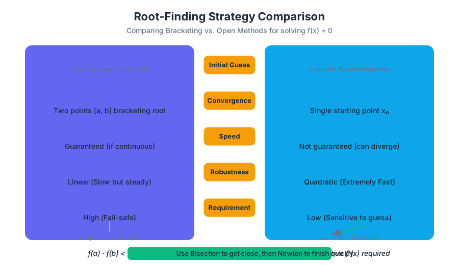
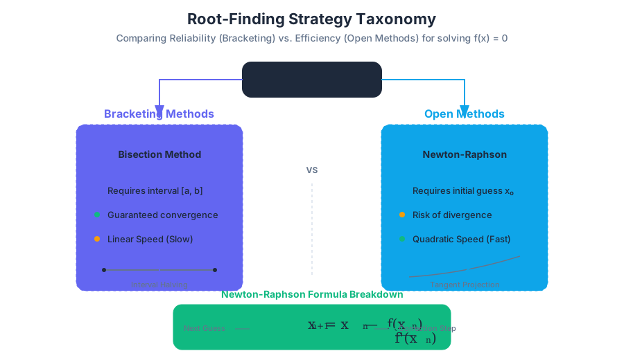
The Mathematical Foundation: Bracketing vs. Open Methods

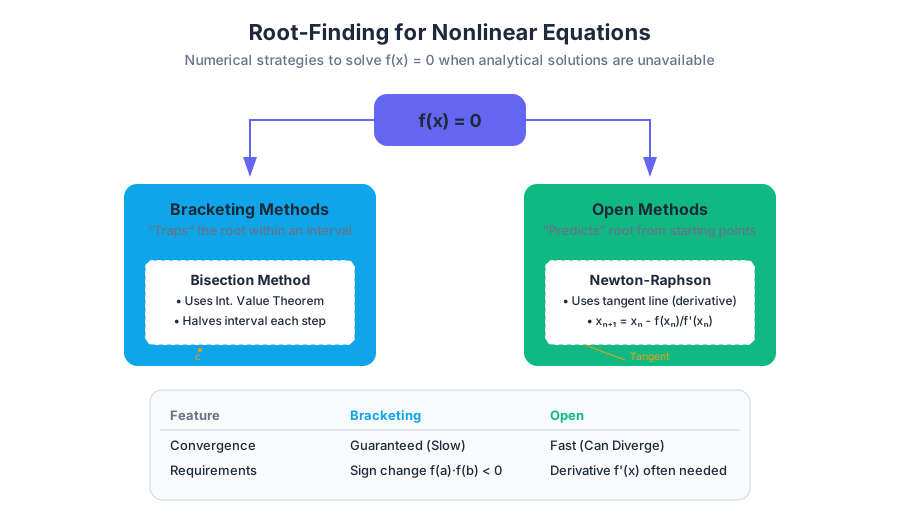
Before diving into specific algorithms, we must categorize root-finding strategies into two main families: Bracketing Methods and Open Methods. This distinction is critical for choosing the right tool for a specific engineering problem.

Feature	Bracketing Methods (e.g., Bisection)	Open Methods (e.g., Newton, Secant)
Initial Guess	Requires two points that bracket the root.	Requires one or two starting points, not necessarily bracketing.
Convergence	Guaranteed to converge if $f(x)$ is continuous.	Not guaranteed; can diverge or oscillate.
Speed	Slow (Linear convergence).	Fast (Quadratic or Superlinear convergence).
Robustness	High; very reliable.	Low; sensitive to the initial guess.
Requirements	$f(a)$ and $f(b)$ must have opposite signs.	May require derivatives ($f'(x)$).

The Intermediate Value Theorem (IVT): If $f(x)$ is a continuous function on the interval $[a, b]$ and $f(a)$ and $f(b)$ have opposite signs (i.e., $f(a) \cdot f(b) < 0$), then there exists at least one root $c$ within the interval $(a, b)$ such that $f(c) = 0$.

---

Bisection Method

The Bisection Method is the numerical equivalent of a binary search. It is a bracketing method that systematically halves an interval to home in on a root.

1. What it is

The Bisection Method is an iterative algorithm that relies on the Intermediate Value Theorem. By repeatedly dividing an interval in half and selecting the sub-interval where the sign change occurs, the method "traps" the root.

2. Why it matters

It is the "fail-safe" of root-finding. While slow, it is mathematically guaranteed to converge to a root if the function is continuous and a valid bracket is provided. It is often used to get a "close enough" guess before switching to a faster method like Newton-Raphson.

3. How it works

1. Start with an interval $[a, b]$ such that $f(a) \cdot f(b) < 0$.
2. Calculate the midpoint $c = \frac{a+b}{2}$.
3. Evaluate $f(c)$.
4. Update the interval:
   • If $f(a) \cdot f(c) < 0$, the root is in $[a, c]$. Set $b = c$.
   • If $f(c) \cdot f(b) < 0$, the root is in $[c, b]$. Set $a = c$.
   • If $f(c) = 0$, $c$ is the exact root.
5. Repeat until the interval width $|b - a|$ is less than a predefined tolerance $\epsilon$.

4. Concrete Example: Solving $f(x) = x^2 - 3$

Let's find $\sqrt{3}$ using the interval $[1, 2]$. Note that $f(1) = -2$ and $f(2) = 1$.

Iteration	$a$	$b$	$c$ (Midpoint)	$f(c)$	Sign Change?
1	1.000	2.000	1.500	-0.750	$[1.5, 2.0]$
2	1.500	2.000	1.750	0.0625	$[1.5, 1.75]$
3	1.500	1.750	1.625	-0.359	$[1.625, 1.75]$
4	1.625	1.750	1.6875	-0.152	$[1.6875, 1.75]$

5. Convergence Analysis

The error at step $n$ is bounded by: $$E_n = \frac{b-a}{2^n}$$ To achieve a specific tolerance $\epsilon$, the number of iterations $n$ required is: $$n > \frac{\ln((b-a)/\epsilon)}{\ln(2)}$$ This confirms linear convergence: each iteration adds roughly 0.301 digits of precision (since $\log_{10}(2) \approx 0.301$).

---

Newton-Raphson Method

The Newton-Raphson Method (often just called Newton's Method) is the gold standard for speed in root-finding, provided you have access to the function's derivative.

1. What it is

Newton's Method is an open method that uses the tangent line of the function at a current guess to predict the location of the root.

2. Why it matters

It converges quadratically, meaning the number of correct digits roughly doubles with each iteration. In high-performance computing, this efficiency is vital.

3. How it works (Derivation)

Consider the Taylor Series expansion of $f(x)$ around the current guess $x_n$: $$f(x_{n+1}) = f(x_n) + f'(x_n)(x_{n+1} - x_n) + \dots$$ Setting $f(x_{n+1}) = 0$ and ignoring higher-order terms, we solve for $x_{n+1}$: $$0 = f(x_n) + f'(x_n)(x_{n+1} - x_n)$$ $$x_{n+1} = x_n - \frac{f(x_n)}{f'(x_n)}$$

4. Implementation in Python

As mentioned in the course materials, Python's simple syntax makes it ideal for implementing these iterative loops.

def newton_method(f, df, x0, tol, max_iter):
    """
    Newton-Raphson for root finding.
    f: function, df: derivative, x0: initial guess
    """
    x = x0
    for i in range(max_iter):
        fx = f(x)
        dfx = df(x)
        
        if abs(dfx) < 1e-12:
            print("Derivative too small; method fails.")
            return None
            
        x_new = x - fx / dfx
        
        if abs(x_new - x) < tol:
            print(f"Converged in {i+1} iterations.")
            return x_new
            
        x = x_new
    return x

# Example: f(x) = x^2 - 2, f'(x) = 2x
root = newton_method(lambda x: x**2 - 2, lambda x: 2*x, 1.5, 1e-7, 100)
print(f"Root: {root}")

5. Common Pitfalls

• Divergence: If the initial guess is far from the root, the method may fly off to infinity.
• Stationary Points: If $f'(x_n) = 0$, the formula involves division by zero.
• Cycles: The method can get stuck in an infinite loop between two values.
• Multiple Roots: If a root has multiplicity $m > 1$ (e.g., $f(x) = (x-1)^2$), convergence drops from quadratic to linear.

---

Secant Method

The Secant Method is a clever modification of Newton's Method designed for cases where the derivative $f'(x)$ is unknown or computationally expensive to calculate.

1. What it is

Instead of using the instantaneous slope (the derivative), the Secant Method uses the slope of a line passing through the two most recent points.

2. Why it matters

It provides a "middle ground" between Bisection and Newton. It is faster than Bisection but doesn't require the symbolic derivative needed for Newton.

3. How it works

We approximate the derivative $f'(x_n)$ using the finite difference: $$f'(x_n) \approx \frac{f(x_n) - f(x_{n-1})}{x_n - x_{n-1}}$$ Substituting this into the Newton-Raphson formula gives the Secant update rule: $$x_{n+1} = x_n - f(x_n) \frac{x_n - x_{n-1}}{f(x_n) - f(x_{n-1})}$$

4. Comparison of Convergence

The Secant Method has a convergence rate of $\phi \approx 1.618$ (the Golden Ratio). It is superlinear, meaning it is faster than Bisection (rate = 1) but slower than Newton (rate = 2).

Method	Convergence Rate ($p$)	Formula for Error $e_{n+1}$
Bisection	1 (Linear)	$e_{n+1} = 0.5 e_n$
Secant	1.618 (Superlinear)	$e_{n+1} = C e_n^{1.618}$
Newton	2 (Quadratic)	$e_{n+1} = C e_n^2$

5. Concrete Example: Solving $f(x) = x^2 - 2$

Initial guesses: $x_0 = 1, x_1 = 2$.

1. $f(1) = -1, f(2) = 2$
2. $x_2 = 2 - 2 \frac{2 - 1}{2 - (-1)} = 2 - 2(1/3) = 1.3333$
3. $f(1.3333) = -0.2222$
4. $x_3 = 1.3333 - (-0.2222) \frac{1.3333 - 2}{-0.2222 - 2} = 1.4000$

---

Convergence Analysis and Stopping Criteria

In practical numerical computing, we rarely find the exact root. Instead, we stop when our approximation is "good enough." Choosing the right stopping criterion is essential to avoid infinite loops or premature termination.

Types of Errors

1. Absolute Error: $|x_{n+1} - x_n| < \epsilon$
2. Relative Error: $\frac{|x_{n+1} - x_n|}{|x_{n+1}|} < \epsilon$ (Preferred when the root magnitude is unknown).
3. Function Tolerance: $|f(x_n)| < \epsilon$ (Ensures the result is actually a "zero").

Comparison Table: Method Selection Matrix

If your function is...	And you have...	Use this method:
Highly unpredictable	Only an interval	Bisection
Smooth and differentiable	A symbolic derivative	Newton-Raphson
Smooth but complex	No symbolic derivative	Secant
A black box	No derivative, limited evals	Brent's Method (Hybrid)

Pro-Tip: In professional libraries (like scipy.optimize), a hybrid approach called Brent's Method is often used. It combines the reliability of Bisection with the speed of inverse quadratic interpolation, switching between them based on the behavior of the function.

---

Practical Pitfalls in Root-Finding

Even with robust algorithms, numerical root-finding can fail in subtle ways.

1. The "Near-Zero" Derivative

In Newton's method, if $f'(x)$ is very small, the step size $\Delta x = f(x)/f'(x)$ becomes massive, shooting the next guess far away from the local region. This is common near local minima or maxima.

2. Multiple Roots

If a function touches the x-axis without crossing it (e.g., $f(x) = x^2$), Bisection will fail because there is no sign change. Newton's method will work but will lose its quadratic convergence, slowing down to linear.

3. Ill-Conditioned Problems

If the function is very "flat" near the root, a large range of $x$ values may satisfy $|f(x)| < \epsilon$. This leads to high uncertainty in the root's location.

4. Floating Point Precision

As discussed in the introductory Python materials, computers have finite precision. If your tolerance $\epsilon$ is smaller than the machine epsilon (typically $\sim 10^{-16}$ for doubles), your loop may never terminate.

Summary of Workflow

To solve a nonlinear equation $f(x)=0$ in a real-world scenario:

1. Plot the function to identify the approximate location of roots and check for discontinuities.
2. Check for derivatives. If $f'(x)$ is easy to compute, use Newton.
3. Establish a bracket. If you need guaranteed convergence, start with Bisection.
4. Implement stopping criteria. Use a combination of relative error and function tolerance.
5. Validate. Plug the result back into $f(x)$ to ensure it is sufficiently close to zero.

Linear Systems and Direct Solvers

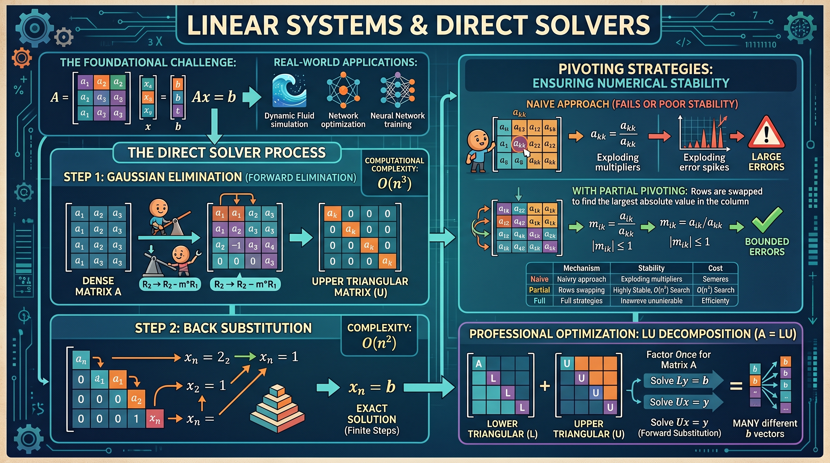
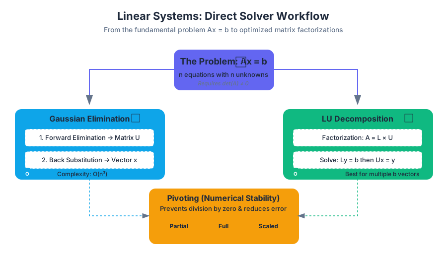
The problem of solving a system of linear equations, represented compactly as $Ax = b$, is the foundational challenge of numerical linear algebra. Whether we are simulating fluid dynamics, optimizing a supply chain, or training a neural network, we eventually encounter a set of linear constraints that must be resolved. In this deep dive, we explore Direct Solvers—algorithms that, in the absence of round-off error, provide an exact solution in a finite number of steps.

The Fundamental Problem: $Ax = b$

At its core, a linear system consists of $n$ equations with $n$ unknowns. We represent this using a matrix $A \in \mathbb{R}^{n \times n}$, a solution vector $x \in \mathbb{R}^n$, and a constant vector $b \in \mathbb{R}^n$.

Definition: A system $Ax = b$ has a unique solution if and only if the matrix $A$ is non-singular. This is equivalent to saying that the determinant $\det(A) \neq 0$, the rank of $A$ is $n$, or that the columns of $A$ are linearly independent.

While Cramer’s Rule provides a theoretical formula for $x$, its computational complexity of $O((n+1)!)$ makes it unusable for any system larger than $3 \times 3$. Direct solvers like Gaussian Elimination and LU Decomposition provide the efficiency required for real-world applications.

---

Gaussian Elimination: The Foundation

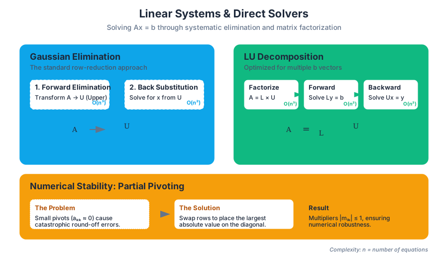
Gaussian Elimination (GE) is the systematic process of applying elementary row operations to transform a dense matrix $A$ into an Upper Triangular Matrix $U$. Once in this form, the system can be solved easily using Back Substitution.

How it Works: The Algorithm

The process is divided into two main phases:

1. Forward Elimination: For each column $k$ from $1$ to $n-1$, we eliminate the entries below the diagonal element $a_{kk}$ (the pivot) in all rows $i > k$. This is done by subtracting a multiple $m_{ik} = a_{ik} / a_{kk}$ of row $k$ from row $i$.
2. Back Substitution: Starting from the last equation (which now has only one unknown), we solve for $x_n$, then substitute it back into the $(n-1)$-th equation to find $x_{n-1}$, and so on.

Computational Complexity

The efficiency of GE is measured in Floating Point Operations (FLOPs).

Phase	Operation Count (Approx.)	Complexity Class
Forward Elimination	$\frac{2}{3}n^3$	$O(n^3)$
Back Substitution	$n^2$	$O(n^2)$
Total	$\frac{2}{3}n^3 + n^2$	$O(n^3)$

Worked Example: Gaussian Elimination

Solve the following system: $$ \begin{aligned} 2x_1 + x_2 + x_3 &= 8 \ -3x_1 - x_2 + 2x_3 &= -11 \ -2x_1 + x_2 + 2x_3 &= -3 \end{aligned} $$

Step 1: Forward Elimination

• Pivot $a_{11} = 2$.
• Eliminate $a_{21}$: $R_2 \leftarrow R_2 - (-3/2)R_1 \implies R_2 \leftarrow R_2 + 1.5R_1$. New $R_2 = [0, 0.5, 3.5, 1]$.
• Eliminate $a_{31}$: $R_3 \leftarrow R_3 - (-2/2)R_1 \implies R_3 \leftarrow R_3 + 1R_1$. New $R_3 = [0, 2, 3, 5]$.

Step 2: Eliminate below new pivot $a_{22} = 0.5$

• $R_3 \leftarrow R_3 - (2/0.5)R_2 \implies R_3 \leftarrow R_3 - 4R_2$.
• New $R_3 = [0, 0, -11, 1]$.

Step 3: Back Substitution

• $-11x_3 = 1 \implies x_3 = -1/11$.
• $0.5x_2 + 3.5(-1/11) = 1 \implies x_2 = 2.636...$
• Substitute $x_2, x_3$ into $R_1$ to find $x_1$.

---

Pivoting Strategies: Ensuring Stability

A naive implementation of Gaussian Elimination fails if a pivot $a_{kk}$ is zero (division by zero) or performs poorly if $a_{kk}$ is very small relative to other elements (leading to massive round-off errors).

Partial Pivoting

To solve this, we use Partial Pivoting. Before eliminating a column, we look at all elements in the current column $k$ at or below the diagonal. We find the element with the largest absolute value and swap its row with the current pivot row.

Theorem: Partial pivoting ensures that the multipliers $m_{ik}$ used in elimination always satisfy $|m_{ik}| \le 1$. This bounds the growth of numerical errors and prevents division by zero in non-singular matrices.

Comparison of Pivoting Techniques

Strategy	Mechanism	Pros	Cons
Naive (None)	Use $a_{kk}$ as is.	Fastest (no searches).	Unstable; fails on zero pivots.
Partial	Swap rows to get max $\vert a_{ik}\vert $ in column.	Highly stable; standard in libraries.	Slight overhead of $O(n^2)$ search.
Full	Swap rows AND columns for max $\vert a_{ij}\vert $.	Most stable possible.	Expensive $O(n^3)$ search; rarely worth it.
Scaled Partial	Pivot based on relative size in row.	Better for poorly scaled rows.	More complex logic.

---

LU Decomposition: The Professional's Choice

In many engineering contexts, we need to solve $Ax = b$ for many different $b$ vectors while $A$ remains the same (e.g., a structural frame under different loading conditions). Gaussian Elimination would require re-processing $A$ every time. LU Decomposition solves this by factoring $A$ into two triangular matrices.

The Factorization

We decompose $A$ such that: $$A = LU$$ Where:

• $L$ is a Lower Triangular matrix (with 1s on the diagonal).
• $U$ is an Upper Triangular matrix (the result of GE).

Solving with LU

Once we have $L$ and $U$, solving $Ax = b$ becomes a two-step process:

1. Solve $Ly = b$ using Forward Substitution.
2. Solve $Ux = y$ using Back Substitution.

Since both $L$ and $U$ are triangular, these steps only take $O(n^2)$ time. The expensive $O(n^3)$ work is done once to find $L$ and $U$.

Python Implementation of LU Decomposition

The following code demonstrates a basic LU decomposition using the Doolittle algorithm.

import numpy as np

def lu_decomposition(A):
    n = len(A)
    L = np.eye(n) # Identity matrix for L
    U = A.copy().astype(float)
    
    for k in range(n):
        for i in range(k + 1, n):
            # Calculate multiplier
            factor = U[i, k] / U[k, k]
            L[i, k] = factor
            # Eliminate entries in U
            U[i, k:] -= factor * U[k, k:]
            
    return L, U

# Example usage
A_mat = np.array([[2, 1, 1],
                  [4, 3, 3],
                  [8, 7, 9]])

L, U = lu_decomposition(A_mat)
print("L:\n", L)
print("U:\n", U)
print("Verification (L @ U):\n", L @ U)

---

Matrix Norms and Condition Numbers

How do we know if our solution $x$ is "good"? In numerical computing, small changes in input (due to measurement error or floating-point precision) can lead to large changes in output. We quantify this using Norms and the Condition Number.

Vector and Matrix Norms

A norm $|x|$ is a measure of the "length" or "size" of a vector or matrix.

Norm Type	Vector Formula ($\Vert x\Vert $)	Matrix Definition ($\Vert A\Vert $)
$L_1$ Norm	$\sum \vert x_i\vert $	Max absolute column sum.
$L_2$ (Euclidean)	$\sqrt{\sum x_i^2}$	Spectral norm (max singular value).
$L_\infty$ Norm	$\max \vert x_i\vert $	Max absolute row sum.

The Condition Number $\kappa(A)$

The condition number measures how sensitive the solution $x$ is to perturbations in $b$.

$$\kappa(A) = |A| \cdot |A^{-1}|$$

• If $\kappa(A) \approx 1$, the matrix is Well-Conditioned.
• If $\kappa(A) \gg 1$, the matrix is Ill-Conditioned.

The Rule of Thumb: If $\kappa(A) = 10^k$, you may lose up to $k$ digits of precision in your solution $x$ beyond what is lost to standard floating-point round-off.

---

Special Cases and Optimized Solvers

Not all matrices require the full $O(n^3)$ treatment. Exploiting matrix structure can lead to significant speedups.

1. Tridiagonal Matrices

In many differential equation solvers, the matrix $A$ only has non-zero entries on the main diagonal and the two adjacent diagonals. The Thomas Algorithm (a simplified version of GE) solves these systems in $O(n)$ time.

2. Symmetric Positive Definite (SPD) Matrices

If $A = A^T$ and $x^T Ax > 0$ for all $x \neq 0$, we can use Cholesky Decomposition: $$A = LL^T$$ This is twice as fast as LU decomposition and numerically more stable, as it does not require pivoting.

3. Summary of Direct Methods

Method	Matrix Requirement	Complexity	Best Use Case
Gaussian Elimination	General Non-singular	$O(n^3)$	Single solve, general $A$.
LU Decomposition	General Non-singular	$O(n^3)$	Multiple $b$ vectors for same $A$.
Cholesky	SPD	$\frac{1}{3}n^3$	Optimization, Physics simulations.
Thomas Algorithm	Tridiagonal	$O(n)$	1D Heat/Wave equations.

---

Common Pitfalls and Troubleshooting

1. The "Singular" Trap: If your solver returns NaN or Inf, check the determinant. If $\det(A) = 0$, the system has no solution or infinite solutions. Direct solvers require a non-singular matrix.
2. Ignoring Pivoting: Never use naive Gaussian Elimination for large systems. Floating-point errors accumulate rapidly; always use a library that implements partial pivoting (like scipy.linalg.solve).
3. The Inverse Mistake: A common novice mistake is calculating $x = A^{-1}b$ by explicitly finding $A^{-1}$.
   • Why it's bad: Computing $A^{-1}$ is more expensive than LU decomposition and usually less numerically stable. Never invert a matrix to solve a linear system. Use a solver.
4. Scaling Issues: If the entries in your matrix differ by many orders of magnitude (e.g., $10^{-10}$ and $10^{10}$), the condition number will explode. Normalize your equations before solving.

Midterm Review and Practice

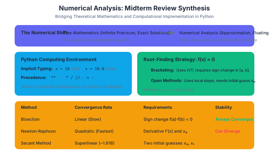
The transition from theoretical mathematics to numerical computing requires a fundamental shift in perspective. In pure mathematics, we often deal with infinite precision and exact solutions; in numerical analysis, we operate in a world of approximations, floating-point arithmetic, and iterative convergence. This midterm review serves as a rigorous synthesis of the first half of the course, bridging the gap between Python implementation and the mathematical bounds that govern algorithmic reliability.

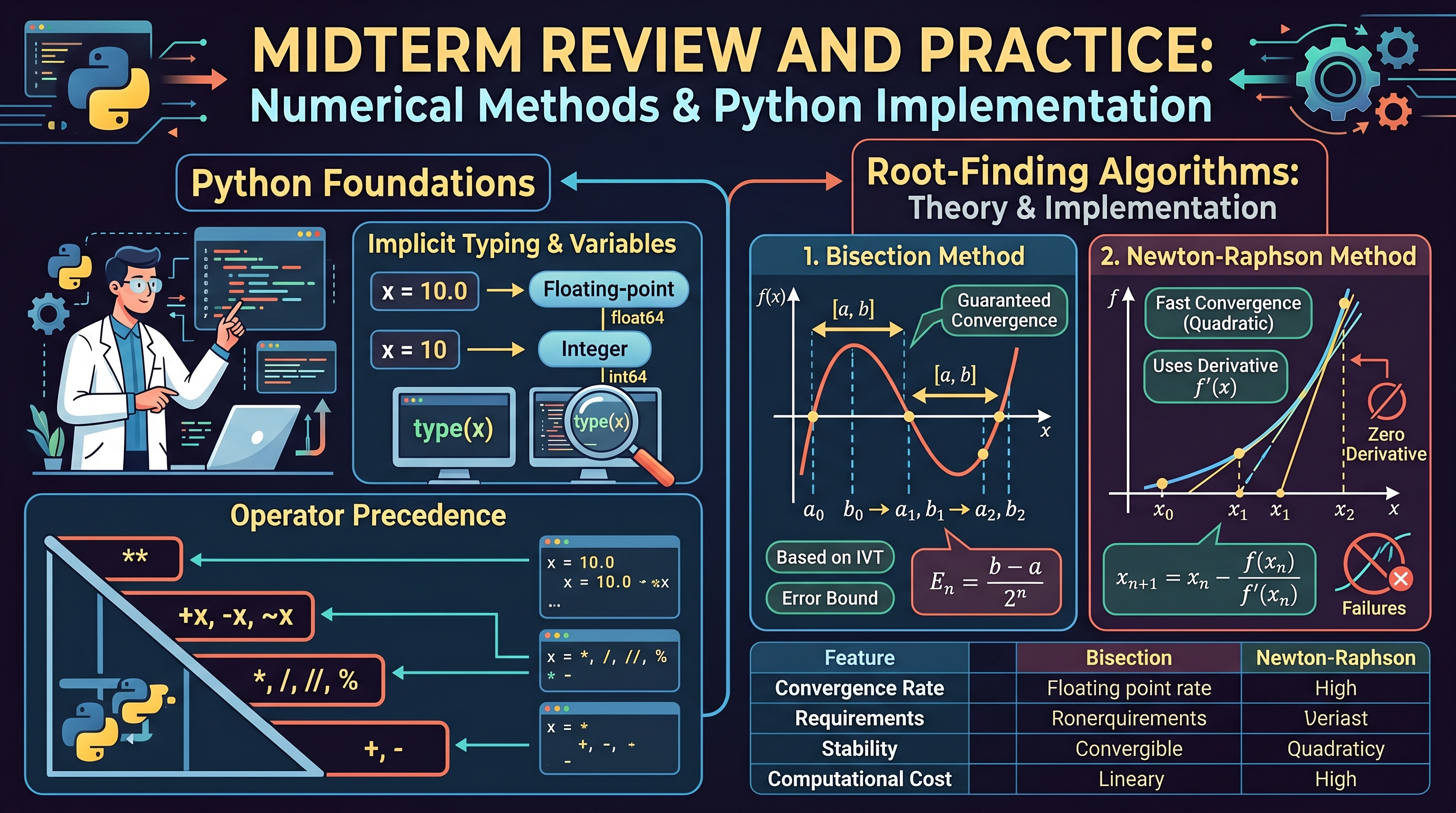
Foundational Computing in Python

Before diving into complex algorithms, a mastery of the computational environment is required. Python serves as our primary vehicle due to its high-level abstraction and robust scientific libraries. Unlike lower-level languages like C++ or Java, Python utilizes implicit typing and dynamic memory management, which allows the researcher to focus on the logic of the numerical method rather than the boilerplate of the machine architecture.

Variable Handling and Type Inference

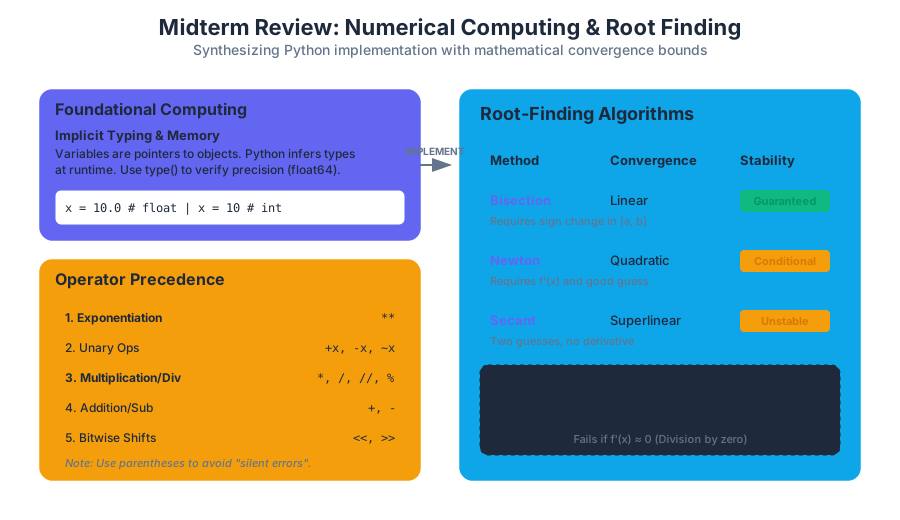
In Python, variables are essentially pointers to objects in memory. When you assign x = 10.0, Python interprets this as a float; x = 10 is interpreted as an integer. For numerical analysis, this distinction is critical because integer division and floating-point division can yield different results in older versions of languages, though Python 3 defaults to float division with the / operator.

The Implicit Typing Rule: Python determines the data type at runtime based on the value assigned. Use the type() function to debug precision issues, especially when dealing with large arrays or matrices where int64 versus float64 can impact memory and result accuracy.

Operator Precedence and Logic

Numerical algorithms often involve complex nested equations. Understanding the order of operations is the first line of defense against "silent errors"—code that runs without crashing but produces the wrong answer.

Precedence	Operator	Description
1 (Highest)	**	Exponentiation
2	+x, -x, ~x	Unary plus, minus, and bitwise NOT
3	*, /, //, %	Multiplication, Division, Floor division, Modulo
4	+, -	Addition, Subtraction
5	<<, >>	Bitwise shifts
6	&	Bitwise AND
7	^	Bitwise XOR
8	|	Bitwise OR
9 (Lowest)	==, !=, >, <, etc.	Comparisons and Identity

---

Root-Finding Algorithms: Theory and Implementation

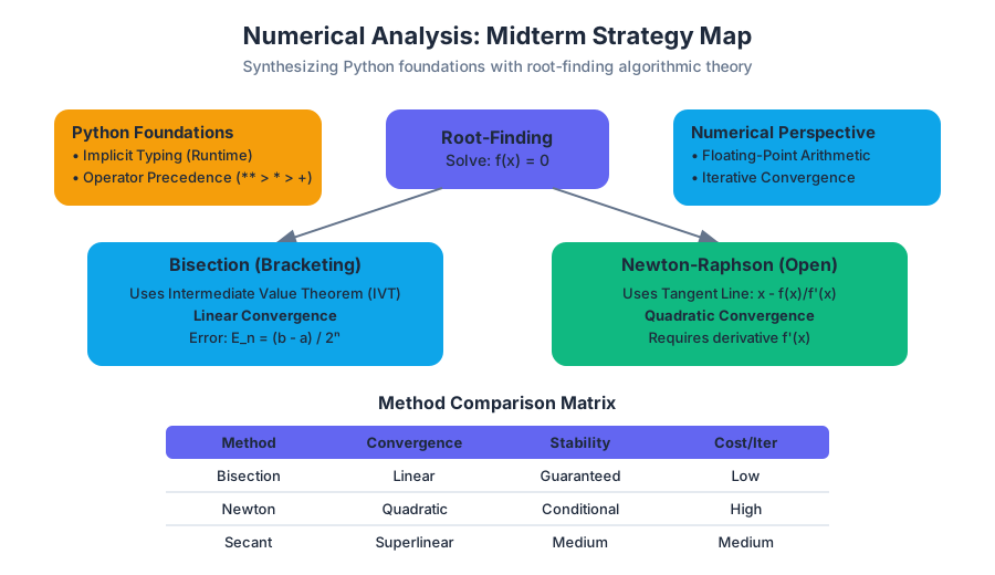
Root-finding is the process of finding a value $x$ such that $f(x) = 0$. This is a cornerstone of numerical computing, used in everything from optimizing structural loads to calculating the internal rate of return in finance.

1. The Bisection Method

The Bisection Method is a "bracketing" method based on the Intermediate Value Theorem. If a continuous function $f(x)$ changes sign over an interval $[a, b]$, a root must exist within that interval.

• How it works: The algorithm repeatedly halves the interval and selects the sub-interval where the sign change occurs.
• Convergence: It is guaranteed to converge if the function is continuous and the initial signs differ. However, it is relatively slow, possessing linear convergence.
• Error Bound: After $n$ iterations, the maximum possible error is: $$E_n = \frac{b - a}{2^n}$$

2. Newton-Raphson Method

The Newton-Raphson Method is an "open" method that uses the derivative of the function to find the root. It approximates the function as a tangent line and finds where that line crosses the x-axis.

• Algorithm: $x_{n+1} = x_n - \frac{f(x_n)}{f'(x_n)}$
• Convergence: When it works, it is extremely fast, exhibiting quadratic convergence ($e_{n+1} \approx Ce_n^2$).
• Pitfalls: It requires the derivative $f'(x)$, and it can fail if $f'(x)$ is zero or if the initial guess $x_0$ is too far from the actual root.

3. Method Comparison for Midterm Preparation

Feature	Bisection Method	Newton-Raphson Method	Secant Method
Convergence Rate	Linear	Quadratic	Superlinear (~1.618)
Requirements	Sign change in $[a, b]$	Initial guess $x_0$, $f'(x)$	Two initial guesses
Stability	Always converges	Can diverge/oscillate	Can diverge
Computational Cost	Low (1 function eval)	High (func + deriv eval)	Medium (1 function eval)

---

Implementation Review: Python Code for Root Finding

In the midterm, you may be asked to identify errors in code or complete a function. Below are the standard implementations for the two primary methods.

def bisection_method(f, a, b, tol, max_iter):
    """
    Implements the Bisection Method to find a root of f(x) = 0.
    """
    if f(a) * f(b) >= 0:
        print("Bisection method fails: Sign does not change.")
        return None
    
    for i in range(max_iter):
        c = (a + b) / 2
        if abs(f(c)) < tol or (b - a) / 2 < tol:
            return c
        
        if f(c) * f(a) < 0:
            b = c
        else:
            a = c
    return (a + b) / 2

def newton_method(f, df, x0, tol, max_iter):
    """
    Implements Newton-Raphson Method.
    f: function, df: derivative of f.
    """
    x = x0
    for i in range(max_iter):
        fx = f(x)
        dfx = df(x)
        
        if abs(dfx) < 1e-12: # Avoid division by zero
            print("Derivative too small; method fails.")
            return None
            
        x_new = x - fx / dfx
        
        if abs(x_new - x) < tol:
            return x_new
        x = x_new
    return x

---

Linear Systems and Gaussian Elimination

Solving systems of linear equations ($Ax = b$) is the "heavy lifting" of numerical analysis. For the midterm, you must understand both the manual trace and the algorithmic complexity.

Gaussian Elimination Steps

1. Forward Elimination: Transform the matrix $A$ into an upper triangular matrix $U$ using row operations.
2. Back Substitution: Solve for the variables starting from the last row.

Pivoting Strategies

Numerical instability occurs when a pivot element (the diagonal element used to eliminate others) is very close to zero. This leads to massive rounding errors.

• Partial Pivoting: Before eliminating a column, swap the current row with the row below it that has the largest absolute value in the pivot column. This is the standard for most robust implementations.

Complexity Analysis

The computational cost of these operations is measured in FLOPS (Floating Point Operations).

Stage	Complexity (Big O)	Notes
Forward Elimination	$O(n^3)$	Dominant cost; involves nested loops.
Back Substitution	$O(n^2)$	Relatively cheap.
Total	$O(n^3)$	Scaling is cubic; doubling $n$ increases time by $8\times$.

---

Error Analysis and Bounds

A numerical solution without an error estimate is often useless. In this course, we categorize errors into three main types:

1. Truncation Error: Arises from approximating a mathematical process (e.g., using a finite Taylor series to represent $e^x$).
2. Round-off Error: Arises from the finite precision of computer memory (e.g., representing $1/3$ as $0.33333333$).
3. Absolute vs. Relative Error:
   • Absolute Error: $|x_{true} - x_{approx}|$
   • Relative Error: $\frac{|x_{true} - x_{approx}|}{|x_{true}|}$

Machine Epsilon ($\epsilon$ ): The smallest positive number such that $1.0 + \epsilon \neq 1.0$. In standard 64-bit floats (double precision), $\epsilon \approx 2.22 \times 10^{-16}$.

Error Bound Calculation Example

If we use the Bisection method on the interval $[1, 2]$ and we want an error less than $10^{-4}$, how many iterations $n$ are required?

Using the formula $E_n = \frac{b-a}{2^n} < \text{tol}$: $$\frac{2-1}{2^n} < 10^{-4}$$ $$1 < 10^{-4} \cdot 2^n$$ $$10^4 < 2^n$$ $$\log_2(10000) < n$$ $$n > 13.28$$ Therefore, 14 iterations are required.

---

Common Exam Patterns and Pitfalls

Based on previous recitations and practice materials, the midterm often focuses on the following "trap" areas:

1. Convergence Failure

• Newton's Method: If the function has a local minimum/maximum near the root, the derivative $f'(x)$ will be near zero, sending the next guess $x_{n+1}$ to infinity.
• Bisection: If the function is tangent to the x-axis (e.g., $f(x) = x^2$), the sign does not change, and Bisection cannot even start.

2. Manual Matrix Tracing

When performing Gaussian Elimination by hand:

• Mistake: Forgetting to apply the row operation to the vector $b$ (the right-hand side).
• Mistake: Sign errors during subtraction ($R_2 = R_2 - m \cdot R_1$).

3. Floating Point Logic

• Comparison: Never use if x == 0.1: in Python. Due to binary representation, 0.1 + 0.2 does not exactly equal 0.3. Always use a tolerance: if abs(x - 0.1) < 1e-9:.

---

Practice Problem Walkthrough

Problem: Find the root of $f(x) = x^3 - x - 1$ using Newton's Method, starting at $x_0 = 1.5$. Perform two iterations.

Step 1: Find the derivative. $f'(x) = 3x^2 - 1$

Step 2: Iteration 1. $f(1.5) = (1.5)^3 - 1.5 - 1 = 3.375 - 1.5 - 1 = 0.875$ $f'(1.5) = 3(1.5)^2 - 1 = 3(2.25) - 1 = 6.75 - 1 = 5.75$ $x_1 = 1.5 - \frac{0.875}{5.75} \approx 1.5 - 0.15217 = 1.34783$

Step 3: Iteration 2. $f(1.34783) \approx (1.34783)^3 - 1.34783 - 1 \approx 2.448 - 1.34783 - 1 = 0.10017$ $f'(1.34783) \approx 3(1.34783)^2 - 1 \approx 3(1.8166) - 1 = 4.4498$ $x_2 = 1.34783 - \frac{0.10017}{4.4498} \approx 1.34783 - 0.02251 = 1.32532$

Analysis: Notice how quickly $f(x)$ approaches zero. In just two steps, the value dropped from $0.875$ to $0.100$. This demonstrates the power of quadratic convergence.

• Bisection Method: A root-finding method that repeatedly bisects an interval and then selects a subinterval in which a root must lie for further processing.
• Newton-Raphson Method: An iterative method for finding the roots of a differentiable function $f$, which are solutions to the equation $f(x) = 0$.
• Gaussian Elimination: An algorithm in linear algebra for solving a system of linear equations, finding the rank of a matrix, and calculating the inverse of an invertible square matrix.
• Partial Pivoting: A technique used in Gaussian elimination to improve numerical stability by swapping rows to ensure the pivot element is the largest possible in its column.
• Relative Error: The ratio of the absolute error of a measurement to the actual measurement.
• Machine Epsilon: The upper bound on the relative error due to rounding in floating-point arithmetic.
• Quadratic Convergence: A property of an iterative method where the number of correct digits roughly doubles with each iteration.
• Forward Elimination: The first phase of Gaussian elimination that reduces a matrix to upper triangular form.
• Back Substitution: The process of solving an upper triangular system of linear equations.
• Truncation Error: The error made by truncating an infinite sum and approximating it by a finite sum.

1. Which method is guaranteed to converge for a continuous function if the initial interval brackets a root?
   • A) Newton-Raphson
   • B) Secant Method
   • C) Bisection Method
   • D) Gaussian Elimination
2. What is the Big O complexity of the Forward Elimination phase in Gaussian Elimination for an $n \times n$ matrix?
   • A) $O(n)$
   • B) $O(n^2)$
   • C) $O(n^3)$
   • D) $O(2^n)$
3. If the absolute error is $0.001$ and the true value is $100$, what is the relative error?
   • A) 0.001
   • B) 0.00001
   • C) 0.1
   • D) 1.0
4. Why is partial pivoting used in Gaussian Elimination?
   • A) To speed up the calculation.
   • B) To reduce the memory footprint.
   • C) To avoid division by zero or very small numbers.
   • D) To make the matrix symmetric.
5. In Python, what is the result of 2 ** 3 * 2?
   • A) 12
   • B) 16
   • C) 64
   • D) 8
6. Which convergence rate is associated with the Newton-Raphson method?
   • A) Linear
   • B) Quadratic
   • C) Cubic
   • D) Logarithmic

Answers: 1-C, 2-C, 3-B, 4-C, 5-B, 6-B.

Midterm Preparation Checklist

• Python Proficiency: Can you write a for loop that implements an iterative sum? Do you understand how if/elif/else blocks control the flow of the Bisection method?
• Root-Finding Mechanics: Practice solving $f(x) = 0$ manually for 2-3 iterations using both Bisection and Newton.
• Error Estimation: Be prepared to solve for $n$ (number of iterations) given a target tolerance and an initial interval.
• Linear Algebra: Practice Gaussian Elimination on a 3x3 matrix. Ensure you can perform back-substitution without calculation errors.
• Method Selection: Know the pros and cons of each method. If a function is expensive to evaluate and you don't have the derivative, which method should you use? (Answer: Secant).
• Conceptual Definitions: Be able to define Machine Epsilon, Truncation Error, and the difference between Absolute and Relative error.
• Code Debugging: Look at a snippet of Gaussian elimination code and identify where the pivoting logic should be inserted.

Iterative Methods for Linear Systems

In the realm of numerical linear algebra, we are often tasked with solving the fundamental equation $Ax = b$. For small systems, direct methods like Gaussian Elimination or LU Decomposition are the gold standard, providing an exact solution (modulo floating-point error) in a predictable number of steps. However, as we transition into the domains of big data, structural engineering, and fluid dynamics, we encounter matrices with millions—or even billions—of rows. In these high-dimensional spaces, direct methods collapse under the weight of $O(n^3)$ computational complexity and massive memory requirements.

This is where Iterative Methods become indispensable. Unlike direct methods that attempt to reach the solution in one multi-step "sweep," iterative methods start with an initial guess $x^{(0)}$ and generate a sequence of approximations $x^{(1)}, x^{(2)}, \dots, x^{(k)}$ that converge toward the true solution.

The Motivation for Iteration: Direct vs. Iterative

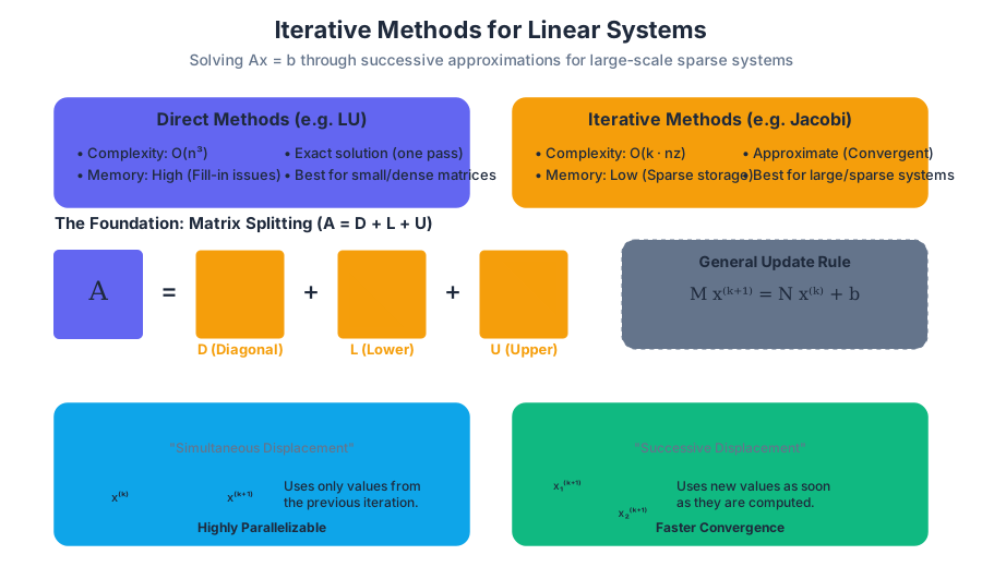
To understand why a professor or senior engineer would choose an iterative approach over a direct one, we must look at the trade-offs in computational "budget." Direct methods are robust but "heavy." Iterative methods are "light" but require specific conditions to ensure they don't wander off into divergence.

Feature	Direct Methods (e.g., LU, QR)	Iterative Methods (e.g., Jacobi, GS)
Complexity	Typically $O(n^3)$	$O(k \cdot n^2)$ or $O(k \cdot nz)$ where $nz$ is non-zeros
Memory Usage	High (suffers from "fill-in")	Low (can operate on sparse formats)
Exactness	Exact (ignoring round-off)	Approximate (controlled by tolerance $\epsilon$)
Suitability	Small to medium dense systems	Large, sparse systems
Stopping Point	Must complete all steps	Can stop early if "good enough"

Key Insight: In many engineering applications, we do not need 16 decimal places of accuracy. If an iterative method can get within $10^{-6}$ of the solution in a few dozen iterations, it is vastly more efficient than waiting hours for a direct solver to finish.

---

The Mathematical Foundation: Matrix Splitting

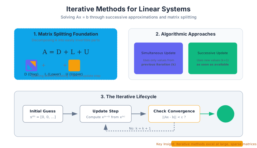
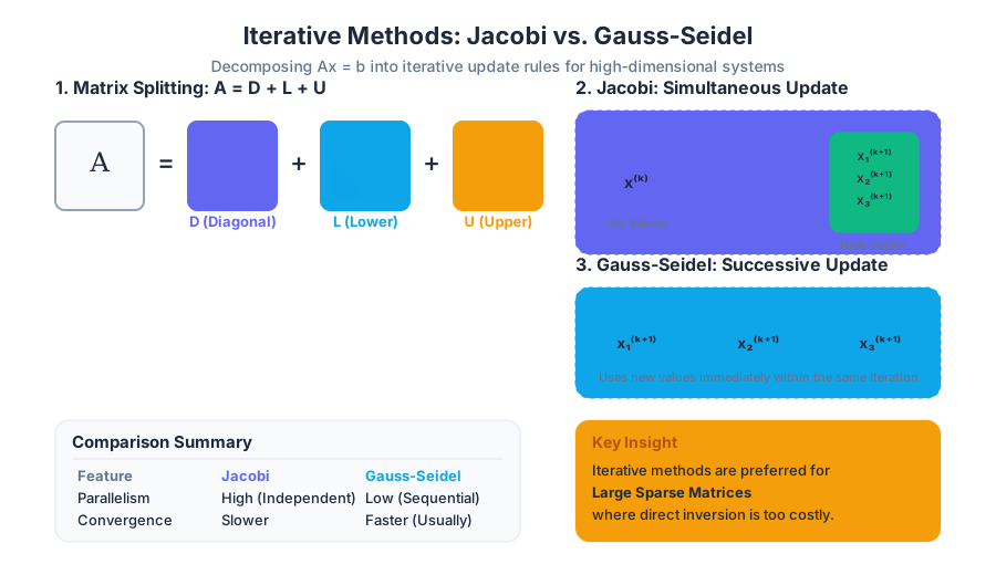
Most classical iterative methods rely on a technique called Matrix Splitting. We decompose the matrix $A$ into parts that are easy to invert. Specifically, we represent $A$ as:

$$A = D + L + U$$

Where:

• $D$ is the Diagonal matrix containing $a_{ii}$.
• $L$ is the Strictly Lower Triangular matrix (elements below the diagonal).
• $U$ is the Strictly Upper Triangular matrix (elements above the diagonal).

By rearranging $Ax = b$ as $(D + L + U)x = b$, we can isolate different components to create an update rule.

---

The Jacobi Method

What it is

The Jacobi Method is the simplest iterative algorithm for solving a system of linear equations. It is a "simultaneous displacement" method, meaning it calculates all components of the new vector $x^{(k+1)}$ using only the values from the previous vector $x^{(k)}$.

How it works

For each row $i$, we solve the equation for the variable $x_i$:

$$x_i^{(k+1)} = \frac{1}{a_{ii}} \left( b_i - \sum_{j \neq i} a_{ij} x_j^{(k)} \right)$$

In matrix form, this is expressed as: $$x^{(k+1)} = D^{-1} (b - (L + U)x^{(k)})$$

Python Implementation

As noted in the course materials, Python's syntax is straightforward. We don't need to declare types; we simply implement the logic using loops or NumPy.

def jacobi(A, b, x0, tolerance, max_iterations):
    n = len(b)
    x = x0.copy()
    x_new = x0.copy()
    
    for k in range(max_iterations):
        for i in range(n):
            sum_j = 0
            for j in range(n):
                if i != j:
                    sum_j = sum_j + A[i][j] * x[j]
            x_new[i] = (b[i] - sum_j) / A[i][i]
        
        # Check for convergence (L2 norm)
        diff = 0
        for i in range(n):
            diff += (x_new[i] - x[i])**2
        if (diff**0.5) < tolerance:
            return x_new
            
        x = x_new.copy()
    return x

Concrete Example

Consider the system: $4x_1 + x_2 = 5$ $x_1 + 3x_2 = 4$

With initial guess $x^{(0)} = [0, 0]^T$:

1. Iteration 1:
   • $x_1^{(1)} = (5 - (1)(0)) / 4 = 1.25$
   • $x_2^{(1)} = (4 - (1)(0)) / 3 = 1.33$
2. Iteration 2:
   • $x_1^{(2)} = (5 - (1)(1.33)) / 4 = 0.9175$
   • $x_2^{(2)} = (4 - (1)(1.25)) / 3 = 0.9166$

The values will eventually converge to the true solution $x = [1, 1]^T$.

---

The Gauss-Seidel Method

What it is

The Gauss-Seidel Method is an evolution of Jacobi. It observes that as soon as we calculate $x_1^{(k+1)}$, it is likely a better approximation than $x_1^{(k)}$. Therefore, we should use it immediately to calculate $x_2^{(k+1)}$, and so on. This is known as the "successive displacement" method.

How it works

The scalar formula incorporates the "new" values as they become available:

$$x_i^{(k+1)} = \frac{1}{a_{ii}} \left( b_i - \sum_{j < i} a_{ij} x_j^{(k+1)} - \sum_{j > i} a_{ij} x_j^{(k)} \right)$$

In matrix form: $$(D + L)x^{(k+1)} = b - Ux^{(k)}$$ $$x^{(k+1)} = (D + L)^{-1} (b - Ux^{(k)})$$

Comparison of Update Logic

Method	Data Usage	Parallelism	Convergence Speed
Jacobi	Uses only "old" data from step $k$	High (all $x_i$ can be computed at once)	Generally slower
Gauss-Seidel	Uses "new" data as soon as it's computed	Low (sequential dependency)	Generally faster

Python Implementation

Note how Gauss-Seidel is actually easier to implement in a memory-efficient way because we can update the vector x in-place.

def gauss_seidel(A, b, x0, tolerance, max_iterations):
    n = len(b)
    x = x0.copy()
    
    for k in range(max_iterations):
        x_old = x.copy()
        for i in range(n):
            sum_j = 0
            for j in range(n):
                if i != j:
                    sum_j = sum_j + A[i][j] * x[j] # Uses current x[j]
            x[i] = (b[i] - sum_j) / A[i][i]
            
        # Convergence check
        error = sum((x[i] - x_old[i])**2 for i in range(n))**0.5
        if error < tolerance:
            return x
    return x

---

Convergence Criteria

Not every matrix $A$ will converge using these methods. If the matrix is "poorly behaved," the iterations might spiral out to infinity.

Strictly Diagonally Dominant (SDD) Matrices

The most common sufficient condition for convergence is Strict Diagonal Dominance.

Definition: A matrix $A$ is Strictly Diagonally Dominant if, for every row $i$, the magnitude of the diagonal element is greater than the sum of the magnitudes of all other elements in that row: $$|a_{ii}| > \sum_{j \neq i} |a_{ij}|$$

If $A$ is SDD, both Jacobi and Gauss-Seidel are guaranteed to converge for any initial guess $x^{(0)}$.

The Spectral Radius

For a more general analysis, we look at the Iteration Matrix $M$. Any iterative method can be written as: $$x^{(k+1)} = Mx^{(k)} + c$$

• For Jacobi: $M_J = -D^{-1}(L+U)$
• For Gauss-Seidel: $M_{GS} = -(D+L)^{-1}U$

Theorem: The iterative method converges if and only if the Spectral Radius $\rho(M) < 1$. The spectral radius is the largest absolute eigenvalue of $M$. The smaller $\rho(M)$, the faster the convergence.

Condition	Impact on Jacobi	Impact on Gauss-Seidel
SDD	Guaranteed Convergence	Guaranteed Convergence
Symmetric Positive Definite	Not Guaranteed	Guaranteed Convergence
$\rho(M) \ge 1$	Divergence	Divergence

---

Sparse Matrices and Efficiency

In modern computing, we rarely store large matrices as 2D arrays. A 1,000,000 x 1,000,000 matrix would require 8 Terabytes of RAM if stored as doubles. However, in many fields, most of these entries are zero. This is a Sparse Matrix.

Why Iterative Methods Win here

Direct methods like LU decomposition create "fill-in." Even if $A$ is sparse, $L$ and $U$ might be dense, destroying our memory efficiency. Iterative methods, however, only require the ability to perform a Matrix-Vector Multiplication ($Ax$).

We can store $A$ in formats like Compressed Sparse Row (CSR):

1. values: Only the non-zero numbers.
2. column_indices: Which column each value belongs to.
3. row_pointers: Where each row starts in the values array.

Complexity Comparison

If a matrix has $n$ rows and an average of $z$ non-zero entries per row:

• Direct Method: $O(n^3)$
• Iterative Method (per iteration): $O(n \cdot z)$

If $z$ is small (e.g., $z=10$ for a 3D mesh), the iterative method is effectively $O(n)$ per iteration. This scalability is why Google's PageRank (an eigenvector problem solved iteratively) and weather simulations are possible.

---

Variations and Extensions: SOR

While Gauss-Seidel is faster than Jacobi, we can accelerate it even further using Successive Over-Relaxation (SOR).

SOR introduces a relaxation parameter $\omega$ (omega): $$x_i^{(k+1)} = (1 - \omega)x_i^{(k)} + \frac{\omega}{a_{ii}} \left( b_i - \sum_{j < i} a_{ij} x_j^{(k+1)} - \sum_{j > i} a_{ij} x_j^{(k)} \right)$$

• If $\omega = 1$: We have standard Gauss-Seidel.
• If $1 < \omega < 2$: We are "over-relaxing," pushing the solution faster toward the limit. This is used to speed up convergence.
• If $0 < \omega < 1$: We are "under-relaxing," which can help stabilize a system that would otherwise diverge.

---

Common Pitfalls and Troubleshooting

1. Zero on the Diagonal: Both Jacobi and Gauss-Seidel involve dividing by $a_{ii}$. If any diagonal element is zero, the method fails immediately. A common fix is Pivoting (swapping rows) before starting the iteration.
2. Slow Convergence: If $\rho(M)$ is very close to 1 (e.g., 0.999), the method may take thousands of iterations to converge. In such cases, preconditioning or switching to Krylov subspace methods (like Conjugate Gradient) is necessary.
3. The "False Convergence" Trap: If your tolerance is too loose, or if the solution is changing very slowly, the algorithm might stop before it reaches the actual solution. Always check the Residual $r = b - Ax^{(k)}$ to ensure the solution actually satisfies the original equation.
4. Ordering Matters: In Gauss-Seidel, the order in which you update $x_i$ affects the results and the rate of convergence. In some specialized hardware (like GPUs), "Red-Black" ordering is used to allow for partial parallelism.

---

Summary of Iterative Workflow

1. Analyze the Matrix: Check for sparsity and diagonal dominance.
2. Choose a Method: Jacobi for parallel systems, Gauss-Seidel for sequential speed, or SOR for optimized performance.
3. Set Parameters: Define a starting guess $x^{(0)}$ (often all zeros), a tolerance $\epsilon$, and a maximum iteration count to prevent infinite loops.
4. Iterate: Update $x$ until the change between steps (or the residual) is below $\epsilon$.
5. Validate: Plug the result back into $Ax = b$ to verify accuracy.