Motion Planning with Graphs of Convex Sets

The Gap Between Discrete and Continuous Planning

In the field of robotic motion planning, a fundamental schism has long existed between two disparate algorithmic philosophies: Discrete Combinatorial Search and Continuous Trajectory Optimization. For decades, practitioners have been forced to choose between the global connectivity guarantees of graph-based methods and the local, dynamically feasible precision of optimization-based methods. This "gap" is not merely a matter of implementation preference; it is a mathematical divide rooted in the topology of configuration spaces ($C$-space) and the computational complexity of navigating non-convex environments.

The challenge arises because the "free space" ($\mathcal{C}_{free}$) in which a robot moves is almost never convex. Obstacles create "holes" or "voids" in the manifold of valid configurations, forcing any planner to make discrete, topological decisions: Do I go left of the pillar or right? Once that discrete decision is made, the problem becomes one of continuous refinement: How do I steer the actuators to follow that path smoothly? Historically, we have solved these two problems sequentially or in isolation, leading to solutions that are either jerky and impractical or smooth but trapped in sub-optimal local minima.

The Discrete Regime: Combinatorial Search and Completeness

Discrete planning treats the world as a collection of nodes and edges. Whether through a predefined grid, a visibility graph, or sampling-based methods like Rapidly-exploring Random Trees (RRT) and Probabilistic Roadmaps (PRM), the goal is to find a sequence of symbolic states that connect a start configuration $q_{start}$ to a goal $q_{goal}$.

Definition: Resolution Completeness A discrete planner is said to be resolution complete if, given a solution exists, the algorithm is guaranteed to find it within a finite amount of time, provided the discretization (grid size or sample count) is sufficiently fine.

The primary advantage of the discrete approach is its ability to handle complex topologies. Because algorithms like Dijkstra’s or A* explore the graph systematically, they do not get "stuck" in the sense that an optimizer does. If a path exists through a narrow corridor, a discrete search will eventually find it. However, this comes at a significant cost:

Feature	Discrete Search (e.g., A*, RRT*)
State Space	Discretized or sampled; loses the "infinitesimal" precision of the real world.
Dynamics	Difficult to incorporate; often requires "kinodynamic" sampling which scales poorly.
Optimality	Only optimal relative to the graph; paths are often "jagged" and require post-processing.
Complexity	Exponential in the dimension of the state space (The Curse of Dimensionality).

The "gap" here is one of quality. A discrete planner might tell you to turn 90 degrees instantly—a physical impossibility for a high-speed drone or a heavy robotic arm. To fix this, we typically "smooth" the path afterward, but this post-processing often pushes the trajectory back into obstacles or violates the very optimality the search was intended to provide.

The Continuous Regime: Trajectory Optimization and Local Minima

On the other side of the divide lies Trajectory Optimization. Here, we represent the robot's path as a continuous function of time, $x(t)$, and attempt to minimize a cost functional $J = \int_{0}^{T} L(x, u) dt$ subject to the robot's nonlinear dynamics $\dot{x} = f(x, u)$ and obstacle constraints $g(x) \leq 0$.

This is typically solved using local methods like Sequential Quadratic Programming (SQP) or Differential Dynamic Programming (DDP). These methods use the gradient of the cost and the Jacobian of the constraints to "push" the trajectory toward a lower-cost, feasible solution.

The Problem of Non-Convexity

The Achilles' heel of continuous optimization is the Local Minimum. Because obstacles are represented as "keep-out" zones, the feasible set of trajectories is non-convex. If an optimizer is initialized on the "wrong" side of an obstacle, the gradient will point it toward the obstacle's surface, where it will get stuck, unable to "jump" to the other side where the global optimum might reside.

The Local Minimum Trap: Imagine a robot trying to reach a goal behind a wall. A local optimizer initialized to go straight will hit the wall and stop, as any small movement left or right might initially increase the distance to the goal or the control effort, creating a "valley" in the cost landscape from which the optimizer cannot escape.

The Mathematical Conflict: NP-Hardness vs. Convexity

Why is this gap so hard to bridge? It comes down to the complexity classes of the underlying math. Finding the shortest path in a non-convex environment is known to be NP-Hard as the number of dimensions increases. Conversely, Convex Optimization is "easy" (solvable in polynomial time) and provides global guarantees.

The gap exists because we are trying to solve an NP-Hard problem (discrete topological choice) using tools designed for convex problems (continuous refinement). Traditional attempts to merge them usually fall into one of two camps:

1. Mixed-Integer Programming (MIP): Formulating the obstacle avoidance as "either/or" constraints. While exact, MIP solvers often struggle with the nonlinear dynamics of robots, leading to massive computation times for even simple tasks.
2. Sampling-based Motion Planning (SBMP): Using discrete samples to "seed" local optimizers. This is the current industry standard (e.g., in the MoveIt! framework), but it lacks the mathematical elegance and robustness of a unified framework.

Bridging the Gap: Graphs of Convex Sets (GCS)

The breakthrough discussed by Russ Tedrake involves a new mathematical framework called Graphs of Convex Sets (GCS). GCS aims to unify the discrete and continuous by rethinking what a "node" in a graph represents. In a traditional graph, a node is a single point. In GCS, a node is a convex set (e.g., a polytope or an ellipsoid) in the configuration space.

The GCS Formulation

In GCS, we decompose the free space $\mathcal{C}_{free}$ into a collection of overlapping convex regions $\mathcal{X}_i$. We then define a graph where:

• Nodes are the convex sets $\mathcal{X}_i$.
• Edges represent the ability to transition from one set to another (usually where sets overlap).
• Continuous Variables $x_i$ are constrained to lie within their respective sets $\mathcal{X}_i$.

The "magic" of GCS is that the problem of finding the shortest path through this graph, while simultaneously optimizing the continuous trajectory within each set, can be formulated as a Convex Optimization problem—specifically, a relaxation of a Mixed-Integer Program that is remarkably tight.

Convex Decomposition: Tiling the Free Space

To use GCS, one must first solve the "Convex Decomposition" problem: how do we turn a complex, non-convex environment into a set of convex polytopes? One leading method is the IRIS (Iterative Regional Inflation by Semidefinite programming) algorithm.

How IRIS Works:

1. Seed Point: Start with a point in $\mathcal{C}_{free}$.
2. Find Nearest Obstacle: Locate the closest point on any obstacle.
3. Hyperplane Separation: Draw a plane (a "tangent") between the seed and the obstacle.
4. Inscribe Ellipsoid: Maximize the volume of an ellipsoid that does not cross any of these planes.
5. Iterate: Use the new ellipsoid to find more obstacles and refine the planes until a large convex "bubble" of free space is formed.

By repeating this process, we can "tile" the entire environment with a finite number of overlapping convex sets. This transforms the infinite complexity of the environment into a finite, combinatorial structure that still preserves the continuous nature of the space.

Method	Representation	Obstacle Handling	Global Optimality
Grid Search	Discrete Pixels/Voxels	Binary Occupancy	Yes (Resolution)
Trajectory Opt	Continuous Splines	Penalty Functions	No (Local Minima)
GCS	Graphs of Convex Sets	Set Constraints	Yes (Global)

The Power of Perspective Functions

The technical core of bridging the gap in GCS involves the use of perspective functions. When we decide whether to "use" an edge in a graph, we usually use a binary variable $z \in {0, 1}$. In standard optimization, this makes the problem non-convex.

However, if we have a convex cost function $f(x)$, we can define its perspective as $g(x, z) = z f(x/z)$. This transformation allows us to "relax" the binary choice. Instead of $z$ being exactly 0 or 1, we let $z$ be anywhere in the interval $[0, 1]$. Because of the properties of perspective functions, the resulting optimization problem remains convex.

This means we can solve for the "flow" of a trajectory through the graph. If the relaxation is tight (which it often is in GCS), the optimizer will naturally push the $z$ values toward 0 or 1, effectively "searching" all possible paths through the obstacles simultaneously and picking the best one—all without ever getting stuck in a local minimum.

Worked Example: Navigating a 2D Maze

Consider a simple 2D robot that needs to move from $(0,0)$ to $(10,10)$ in a room with a large central obstacle.

1. Decomposition: Using IRIS, we generate four convex polytopes (rectangles) that cover the free space around the central obstacle. Let's call them $S_{North}, S_{South}, S_{East}, S_{West}$.
2. Graph Construction: We create edges between sets that overlap. For example, $S_{West}$ overlaps with $S_{North}$ and $S_{South}$.
3. Cost Definition: We define our cost as the squared Euclidean distance: $\sum |x_{i+1} - x_i|^2$.
4. Optimization: We solve the GCS problem. The optimizer doesn't just "try" the North path. It looks at the entire graph of sets. It evaluates the minimum possible cost of traversing ${S_{West} \to S_{North} \to S_{East}}$ versus ${S_{West} \to S_{South} \to S_{East}}$.
5. Result: Because the formulation is convex, the solver returns the mathematically guaranteed shortest path that respects the boundaries of the rectangles.

In a traditional optimizer, if you started the robot slightly closer to the South, it would be forced to take the South path. In GCS, even if you start near the South, if the North path is 1% shorter, the solver will find it.

Common Pitfalls and Limitations

While GCS and similar convex-bridging methods are powerful, they are not magic bullets. Senior engineers should be aware of several critical nuances:

• Decomposition Quality: The efficiency of the search depends heavily on the convex decomposition. If the sets are too small or too numerous, the resulting graph becomes massive, slowing down the solver. If they are too large, they might not capture the nuances of the environment.
• High-Dimensional Dynamics: While GCS handles kinematics beautifully, incorporating full nonlinear dynamics (like the aerodynamics of a flapping wing) still requires approximations. Often, we use "flat" outputs or mixed-integer formulations that can become computationally expensive.
• The Relaxation Gap: Although the GCS relaxation is "tight," it is not always perfect. In some edge cases, the solver might return a "fractional" solution where the robot seems to exist in two paths at once. Rounding these solutions back to a valid path requires careful algorithmic handling.

Summary of the Integrated Approach

The "Gap" between discrete and continuous planning is being closed by moving away from the "Search then Optimize" pipeline toward a "Search via Optimization" framework. By encoding the discrete topology of the world into the constraints of a convex program, we gain the best of both worlds: the reliability of a map and the elegance of a smooth curve.

As robotics moves toward more safety-critical applications—such as autonomous surgery or high-speed urban drone delivery—the ability to provide global guarantees on trajectory optimality and feasibility becomes not just a theoretical luxury, but a fundamental requirement.

The GCS Mathematical Framework

The Graphs of Convex Sets (GCS) framework represents a paradigm shift in robotic motion planning, effectively bridging the historical divide between discrete graph-search algorithms (like A* or Dijkstra) and continuous trajectory optimization (like Sequential Quadratic Programming). Traditionally, motion planning was forced into a trade-off: one could either search a graph of discrete states to find a globally optimal path that ignores complex dynamics, or use local optimization to find a dynamically feasible trajectory that is prone to getting stuck in local minima. GCS provides a unified mathematical structure that allows for global optimization over continuous paths through a series of convex regions.

At its core, GCS formulates the motion planning problem as a Shortest Path Problem on a Graph of Convex Sets. In this formulation, vertices are not single points in space but rather entire convex regions (such as polytopes or ellipsoids) of the configuration space. Edges represent the transitions between these regions. The "cost" of an edge is not a fixed scalar but a convex function of the continuous variables (the path) within those sets. This allows the framework to solve for the discrete sequence of regions and the continuous trajectory simultaneously, often reaching the global optimum via convex relaxation.

Convex Decomposition: Mapping the Free Space

Before a GCS problem can be solved, the robot's configuration space ($C_{free}$) must be represented as a collection of convex sets. This process, known as Convex Decomposition, is the geometric foundation of the framework. Because collision-avoidance constraints are inherently non-convex (obstacles create "holes" in the space), we cannot optimize over the entire space at once. Instead, we decompose the free space into a set of overlapping convex regions where $x \in \mathcal{X}_i$.

The primary tool for this decomposition in the GCS ecosystem is the IRIS (Iterative Regional Inflation by Semidefinite programming) algorithm. IRIS seeks to find the largest possible convex polytopes that do not contain any obstacles. The algorithm alternates between two main steps:

1. Finding Separating Hyperplanes: Given an ellipsoid, find the planes that best separate the ellipsoid from the obstacles.
2. Updating the Maximum Inscribed Ellipsoid: Given the hyperplanes, find the largest ellipsoid that fits within the resulting polytope.

Definition: Convex Polytope A convex polytope $\mathcal{P}$ is defined as the intersection of a finite number of half-spaces, represented mathematically as ${x \in \mathbb{R}^n \mid Ax \le b}$, where $A$ is a matrix of normal vectors and $b$ is a vector of offsets.

Feature	Polytopes ($Ax \le b$)	Ellipsoids ($(x-c)^T Q (x-c) \le 1$)	Voxel Grids
Representational Power	High (can fit complex walls)	Moderate (smooth)	Low (blocky)
Constraint Type	Linear Inequalities	Quadratic Constraints	Discrete Lookups
Optimization Fit	Excellent for Linear/Quadratic Programs	Good for SOCP	Poor for Continuous Opt
Overlap Handling	Easy to compute intersections	Computationally heavier	Trivial

The choice of convex sets is critical. If the sets are too small, the graph becomes excessively large, increasing the combinatorial complexity. If the sets are too large or poorly placed, they may fail to capture the connectivity of a narrow passage. The goal is a "sparse but covering" decomposition where the union of the sets $\bigcup \mathcal{X}i$ covers as much of $C{free}$ as possible.

The Shortest Path Problem on GCS

Once the space is decomposed, we define a graph $G = (V, E)$. Each vertex $v \in V$ is associated with a convex set $X_v \subseteq \mathbb{R}^n$. An edge $e = (u, v) \in E$ exists if the robot can transition from set $X_u$ to set $X_v$. Unlike a standard graph where an edge has a weight $w_{uv}$, a GCS edge has a cost function $J_e(x_u, x_v)$ and constraints on the continuous variables $x_u \in X_u$ and $x_v \in X_v$.

The mathematical objective is to find a sequence of edges (a path) and the specific points within each set along that path that minimize the total cost: $$\min \sum_{e \in \text{Path}} J_e(x_u, x_v)$$ subject to:

• $x_v \in X_v$ (Set membership)
• $(x_u, x_v) \in \mathcal{C}_e$ (Transition constraints, such as continuity or dynamics)
• The path must start at $x_{start}$ and end at $x_{goal}$.

This problem is inherently a Mixed-Integer Convex Program (MICP). The "integer" part comes from the discrete decision of which edges to include in the path (binary variables $z_e \in {0, 1}$), and the "convex" part comes from the optimization of $x$ within the chosen sets.

Perspective Functions: The Key to Convex Relaxation

The most significant mathematical innovation in GCS is the use of Perspective Functions to create a "tight" convex relaxation of the MICP. In a standard Mixed-Integer problem, if we simply relax the binary variables $z_e \in {0, 1}$ to continuous variables $z_e \in [0, 1]$, the resulting optimization often yields "weak" bounds, meaning the solution to the relaxed problem is far from the true integer solution.

To solve this, GCS employs the Perspective of the convex constraints. For a convex function $f(x)$, the perspective function is defined as: $$g(x, z) = z f(x/z)$$ where $z$ is the relaxation of the binary indicator variable.

Why the Perspective Matters

Consider a constraint $x \in \mathcal{X}$ where $\mathcal{X}$ is a convex set. If the edge is "off" ($z=0$), we want $x$ to be forced to zero (or some null value) so it doesn't contribute to the cost. If the edge is "on" ($z=1$), we want the original constraint $x \in \mathcal{X}$ to apply. The perspective transformation $z (A(x/z)) \le z b$, which simplifies to $Ax \le zb$, achieves exactly this. When $z=1$, we get $Ax \le b$. When $z=0$, we get $Ax \le 0$, which (for many sets) forces $x=0$.

Theorem: Convex Hull of the Union of Sets The perspective formulation is mathematically equivalent to finding the Convex Hull of the union of the individual convex constraints. This is the "tightest" possible convex representation of a discrete choice between convex sets.

Mixed-Integer Programming vs. Convex Relaxation

The GCS framework allows the user to choose between solving the exact MICP (which is NP-hard but yields the absolute global optimum) or solving the convex relaxation (which is polynomial time). Remarkably, for many motion planning problems, the convex relaxation is exact or "tight," meaning the $z_e$ variables naturally come out as 0 or 1, or can be easily rounded to a valid path.

Approach	Complexity	Optimality	Use Case
Pure Graph Search (A)*	$O(V \log V + E)$	Global (Discrete)	High-level routing, no dynamics
Trajectory Opt (SQP)	$O(Iteration \times N^3)$	Local	Refining a known path
GCS (MICP)	Exponential (Worst case)	Global (Continuous)	Complex environments, high stakes
GCS (Relaxation)	Polynomial	Often Global	Real-time planning, large graphs

The "tightness" of the GCS relaxation stems from the fact that we are not just relaxing the binary variables, but we are lifting the continuous variables into a higher-dimensional space where the union of the convex sets is represented by its convex hull. This is a much stronger formulation than the "Big-M" method often used in older mixed-integer formulations.

Implementation: The GCS Pipeline

A senior engineer implementing GCS for a robotic system (such as a manipulator or a humanoid) follows a specific mathematical pipeline. This pipeline ensures that the resulting trajectory is not only collision-free but also satisfies the dynamic limits of the robot.

1. Decomposition: Run IRIS to generate a set of polytopes $\mathcal{P}_i$ that cover the free configuration space.
2. Graph Construction: Create vertices for each $\mathcal{P}_i$. Create edges between vertices if $\mathcal{P}_i \cap \mathcal{P}_j \neq \emptyset$.
3. Constraint Specification: For each edge, define the continuity constraints. For example, if $x$ represents a spline, ensure that the position and velocity at the end of $x_u$ match the start of $x_v$.
4. Cost Definition: Define the objective function, typically a quadratic cost like $\int |\ddot{x}(t)|^2 dt$ to minimize control effort (jerk/acceleration).
5. Solve Relaxation: Solve the resulting large-scale convex program (usually a Second-Order Cone Program or SOCP).
6. Rounding (if necessary): If the relaxation returns fractional $z_e$ values, use a k-shortest path algorithm on the graph weights to extract the best discrete path, then solve the resulting fixed-path convex optimization.

Worked Example: 2D Point Robot

Imagine a point robot moving from $(0,0)$ to $(10,10)$ with a large obstacle in the middle.

• Sets: We decompose the space into four overlapping rectangles: $S_1$ (bottom-left), $S_2$ (top-left), $S_3$ (bottom-right), $S_4$ (top-right).
• Edges: $E = {(S_1, S_2), (S_1, S_3), (S_2, S_4), (S_3, S_4)}$.
• Decision: The solver must choose between the path $S_1 \to S_2 \to S_4$ or $S_1 \to S_3 \to S_4$.
• Perspective: The solver evaluates the "flow" $z_e$ through these edges. Because the perspective formulation is used, the solver "sees" the cost of the optimal continuous trajectory within each path during the discrete search.

Variations and Extensions

The GCS framework is highly extensible. Beyond simple point-to-point planning, it has been adapted for several complex robotic tasks:

• Dynamic Constraints: By representing the trajectory as a B-spline, the derivatives (velocity, acceleration) are also linear functions of the control points. This allows GCS to enforce limits on speed and torque while remaining a convex problem.
• Task and Motion Planning (TAMP): GCS can handle discrete changes in the environment, such as picking up an object. The "sets" in this case represent different modes of the system (e.g., "Robot moving," "Robot carrying object").
• Time-Optimal Planning: While minimizing time is non-convex, GCS can be used with a "time-scaling" approach where the path is fixed and the timing is optimized, or by performing a line search over the total duration.

Common Pitfalls and Misconceptions

While GCS is powerful, it is not a "silver bullet." Engineers often encounter specific hurdles during implementation:

• The "Over-Segmentation" Problem: If the convex decomposition creates too many tiny sets, the number of binary variables in the MICP grows, and even the relaxation can become slow to solve. Efficient decomposition is as important as the solver itself.
• Numerical Conditioning: The perspective function $z f(x/z)$ involves division by $z$. As $z \to 0$, this can lead to numerical instability in solvers. Practical implementations use a small epsilon ($z + \epsilon$) or specialized conic solver formulations to handle this.
• Completeness: GCS is "resolution-complete" with respect to the convex decomposition. If a path exists through the union of the sets, GCS will find it. However, if the IRIS decomposition misses a narrow gap, GCS will not find a path through that gap.

Key Insight: GCS is not just a new algorithm; it is a new way of writing down the motion planning problem so that modern, high-performance convex solvers (like Mosek or Gurobi) can do the heavy lifting. It moves the complexity from the "search logic" to the "mathematical formulation."

Convex Relaxations and Tightness

In the landscape of modern robotics and motion planning, the "holy grail" has long been an algorithm that combines the global optimality of discrete graph search with the dynamic feasibility of continuous trajectory optimization. Historically, these two worlds were separated by a computational chasm: discrete search (like A*) handles combinatorial complexity but struggles with high-dimensional dynamics, while continuous optimization (like SQP) handles dynamics but gets trapped in local minima created by obstacles. The Graphs of Convex Sets (GCS) framework, as introduced by Russ Tedrake and his team, bridges this chasm by reformulating motion planning as a convex optimization problem over a graph. Central to the success of this approach is the concept of Convex Relaxations and their Tightness—the mathematical property that allows us to solve NP-hard combinatorial problems with the efficiency of simple convex programs.

The Combinatorial Challenge: Mixed-Integer Programming (MIP)

To understand why convex relaxations are necessary, we must first acknowledge the inherent difficulty of motion planning around obstacles. When a robot encounters an obstacle, it faces a binary choice: go left or go right. In mathematical terms, this is an "either/or" constraint, which is non-convex. The standard way to model such decisions is through Mixed-Integer Programming (MIP). In a MIP, some variables are constrained to be integers (usually binary, $y \in {0, 1}$), representing discrete choices, while others are continuous ($x \in \mathbb{R}^n$), representing positions or velocities.

Definition: Mixed-Integer Program (MIP) A MIP is an optimization problem of the form: $$\min_{x, y} f(x, y)$$ subject to: $$g(x, y) \leq 0$$ $$x \in \mathbb{R}^n, y \in {0, 1}^m$$ Where $y$ represents the discrete decisions (e.g., "Am I in region A or region B?") and $x$ represents the continuous state.

While MIPs are incredibly expressive, they are generally NP-hard. Solving them typically requires a "Branch and Bound" approach, which explores a search tree of binary decisions. In the worst case, the number of branches grows exponentially with the number of obstacles, making real-time motion planning for complex environments computationally prohibitive.

Feature	Mixed-Integer Programming (MIP)	Standard Nonlinear Optimization
Decision Type	Discrete + Continuous	Continuous Only
Global Optimality	Guaranteed (given enough time)	Not Guaranteed (local minima)
Complexity	Exponential (NP-hard)	Polynomial (usually)
Obstacle Handling	Exact (via binary variables)	Heuristic (via penalty functions)

Defining Convex Relaxation

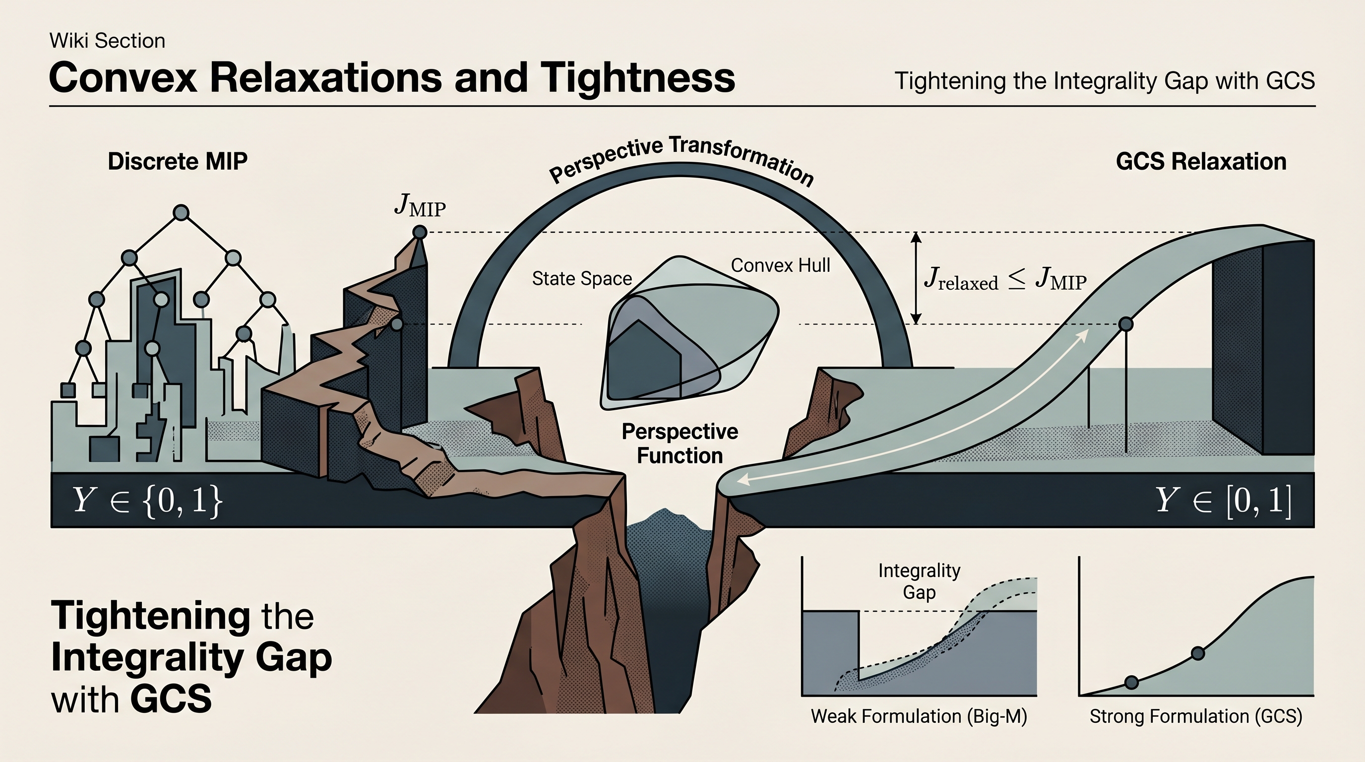
A Convex Relaxation is the process of taking a hard, non-convex problem and replacing it with a simpler, convex one that "contains" the original. In the context of GCS, we relax the binary constraint $y \in {0, 1}$ to a continuous interval constraint $y \in [0, 1]$. This transformation turns a combinatorial search into a continuous optimization problem that can be solved in polynomial time using interior-point methods.

Mathematically, if the original feasible set is $S$, the relaxation seeks a convex set $\hat{S}$ such that $S \subseteq \hat{S}$. The goal is to find the "tightest" possible $\hat{S}$—the one that most closely hugs the original non-convex set. If the relaxation is perfectly tight, the optimal solution to the relaxed problem will naturally land on an integer value (0 or 1), even though it was allowed to be anything in between.

The Integrality Gap

The quality of a relaxation is measured by the Integrality Gap. This is the difference between the objective value of the optimal integer solution ($J_{MIP}$) and the objective value of the relaxed solution ($J_{relaxed}$). Since the relaxed problem is less constrained, its optimal value is always less than or equal to the true integer optimum: $$J_{relaxed} \leq J_{MIP}$$

A gap of zero implies that the relaxation is tight. In GCS, the objective is to formulate the graph search such that the integrality gap is zero or near-zero, allowing the solver to find the globally optimal path without ever explicitly "branching" on the binary variables.

Strong Formulations and the Perspective Function

Not all relaxations are created equal. A "weak" formulation might satisfy the constraints but result in a large integrality gap, leading the solver to produce "fuzzy" solutions where a robot is 50% in one region and 50% in another. To achieve Tightness, GCS utilizes what is known in the optimization community as a Strong Formulation.

The secret to the GCS "strength" is the use of the Perspective Function. When we associate a continuous variable $x$ (like a position) with a binary variable $y$ (representing whether we are in a specific convex set $X$), we don't just say $x \in X$ if $y=1$. Instead, we use a higher-dimensional representation: $$x \in yX$$ Where $yX$ is the scaling of the set $X$ by the factor $y$. If $y=1$, the constraint is $x \in X$. If $y=0$, the constraint collapses to $x=0$.

The Mathematical Derivation

If a convex set is defined by the inequalities $Ax \leq b$, the perspective of that set is defined by: $$A(x/y) \leq b \implies Ax \leq by$$ This transformation is crucial because the set of points $(x, y)$ satisfying $Ax \leq by$ for $y \in [0, 1]$ is itself a convex cone. By summing these perspective-based constraints across all edges and vertices in the graph, GCS creates a formulation that is the convex hull of the original shortest-path problem.

Formulation Type	Mechanism	Tightness	Solver Performance
Big-M Formulation	$x \leq M \cdot y$	Weak	Slow convergence, large gaps
Convex Hull (GCS)	$Ax \leq by$	Strong	Fast convergence, often zero gap
Penalty Methods	$\lambda \cdot \text{dist}(x, X)$	Very Weak	Prone to local minima

The Dual Problem: Potentials and Lower Bounds

In optimization, every primal problem (the one we want to solve) has a Dual Problem. For GCS, the dual problem provides deep insights into why the relaxation is so effective. In the context of a graph, the dual variables can be interpreted as Potentials at each vertex.

If we are looking for the shortest path from a start vertex $s$ to a goal vertex $t$, the dual problem is essentially trying to find the largest possible lower bound on the cost-to-go. In a standard graph, this is equivalent to the Bellman equation. In GCS, because each node is a convex set, the dual variables represent "cost-to-go functions" over those sets.

Key Insight: The Dual as a Certificate The dual problem provides a "certificate" of optimality. If the value of the dual objective matches the value of the primal objective, we have proof that we have found the global optimum. Because the GCS relaxation is so tight, the dual bound is often extremely high, which allows the solver to prune large sections of the graph that cannot possibly contain the optimal solution.

Dual Variables in GCS:

1. $\phi_v$: The potential at vertex $v$.
2. $\lambda_{uv}$: The dual variables associated with the edges.
3. Interpretation: The dual problem maximizes the potential at the start node subject to the constraint that the potential difference between nodes cannot exceed the cost of the edge connecting them.

Why GCS is "Tight" in Practice

One of the most surprising results presented by Russ Tedrake is that for many motion planning problems, the GCS relaxation is exactly tight. This means the solver returns an integer solution ($y=0$ or $y=1$) directly, without any rounding or branching.

This tightness stems from the fact that the GCS formulation is the convex hull of the flow constraints on a graph. In classical network flow theory, the "Shortest Path Problem" on a graph is known to have a Totally Unimodular (TU) constraint matrix. TU matrices have the magical property that their vertices are always integers. While the addition of convex set constraints (the "continuous" part) breaks pure TU, the "Strong Formulation" using perspective functions preserves much of this structure, keeping the integrality gap at or near zero for a wide class of problems.

Factors Influencing Tightness:

• Set Overlap: If convex sets overlap significantly, the relaxation remains strong.
• Cost Function: Linear or convex quadratic costs (like squared distance) tend to preserve tightness.
• Graph Topology: Cycles in the graph can sometimes introduce gaps, but GCS handles this by enforcing flow conservation.

Worked Example: Navigating a "U-Shaped" Obstacle

Consider a robot that must move from $(0,0)$ to $(10,10)$ but must pass around a large U-shaped obstacle. A standard nonlinear optimizer would likely drive the robot into the "pocket" of the U and get stuck in a local minimum.

1. Decomposition: We decompose the free space into three overlapping convex sets: $X_1$ (left of the U), $X_2$ (right of the U), and $X_3$ (above the U).
2. Graph Construction: We create a graph where vertices are these sets. Edges exist where sets overlap.
3. MIP Formulation: We define binary variables $y_{12}, y_{23}$, etc., to represent the path taken.
4. Relaxation: We relax $y \in [0, 1]$ and apply the perspective transformation to the dynamics.
5. Execution: The solver (e.g., Mosek or Gurobi) sees a single large convex problem. It evaluates the "cost-to-go" through the left path vs. the right path simultaneously in a continuous space.
6. Result: Because the formulation is tight, the solver identifies that the left path is $2.5$ units shorter and returns $y_{left}=1, y_{right}=0$. The robot follows the globally optimal trajectory without ever "seeing" the local minimum inside the U.

Step	Action	Mathematical Tool
1	Identify Obstacles	Configuration Space Analysis
2	Partition Space	Convex Decomposition (IRIS)
3	Define Costs	Quadratic/Convex Objectives
4	Solve Relaxation	Interior-Point Method (Convex)
5	Extract Path	Integrality Check / Rounding

Common Pitfalls and Misconceptions

While GCS and its relaxations are powerful, they are not magic. Users often encounter specific hurdles:

• The "Big-M" Trap: Many engineers attempt to implement GCS using "Big-M" constraints (e.g., $x \leq 1000 \cdot y$). This is mathematically valid but numerically disastrous. It leads to very weak relaxations and slow solver performance. Always use the perspective formulation ($Ax \leq by$).
• Non-Convex Costs: If the cost function itself is non-convex (e.g., minimizing time in a system with non-linear dynamics), the relaxation may no longer be convex. GCS requires the cost within each set to be convex.
• Over-Decomposition: While more convex sets make the approximation of free space more accurate, they also increase the number of variables in the optimization. There is a trade-off between geometric fidelity and computational speed.
• Numerical Precision: Because perspective functions involve terms like $x/y$, they can become numerically unstable as $y \to 0$. High-quality solvers handle this using specialized "rotated second-order cone" constraints to maintain stability.

Applications and Performance in Robotics

The field of motion planning has long been bifurcated into two distinct philosophies: discrete graph search and continuous trajectory optimization. While graph search algorithms like A* or RRT* are excellent at navigating complex combinatorial mazes, they often struggle with high-dimensional dynamics and smoothness. Conversely, trajectory optimization excels at producing fluid, dynamically feasible motions but is notoriously susceptible to local minima in cluttered environments. Graphs of Convex Sets (GCS), as introduced by Russ Tedrake and his team, represents a unified framework that bridges this gap. By formulating the motion planning problem as a shortest path problem over a graph of convex sets, GCS provides a powerful tool for generating globally optimal, dynamically feasible trajectories for a wide array of robotic systems, from agile UAVs to complex humanoid walkers.

The GCS Framework: Unifying Discrete and Continuous Planning

At its core, GCS addresses the challenge of planning in a space that is both continuous (the robot's configuration) and discrete (the sequence of regions or "corridors" the robot must pass through). In traditional methods, one might use a graph search to find a sequence of collision-free regions and then use optimization to "smooth" a path through them. However, this decoupled approach often fails to find the true global optimum because the initial discrete choice might preclude the most efficient continuous trajectory.

Definition: Graph of Convex Sets (GCS) A GCS is a mathematical structure where nodes represent convex sets $X_i \subseteq \mathbb{R}^n$ (typically representing safe regions in configuration space) and edges represent transitions between these sets. The goal is to find a continuous trajectory $x(t)$ that starts in a source set, ends in a target set, and minimizes a cost function while remaining within the union of the sets and satisfying dynamical constraints.

The breakthrough of GCS lies in its mathematical formulation. By using the perspective function of convex costs and constraints, the problem can be formulated as a Mixed-Integer Convex Program (MICP). More importantly, the convex relaxation of this MICP is remarkably tight, often providing the exact global optimum in polynomial time for many practical robotics problems.

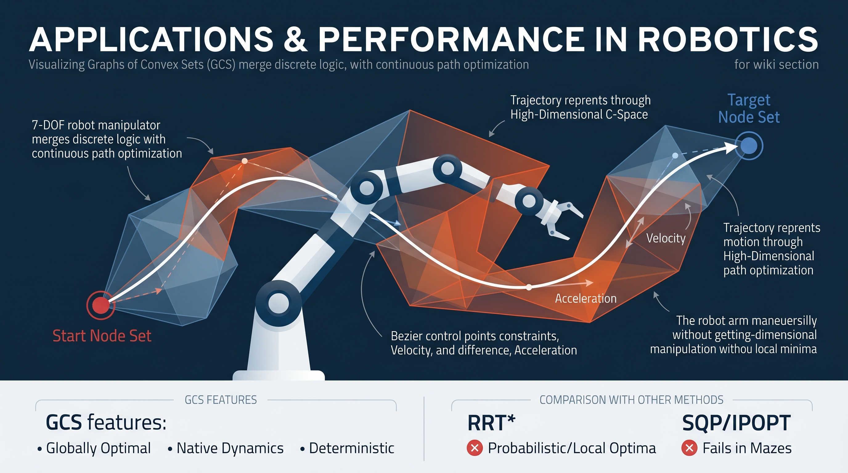
Feature	Sampling-Based (RRT*)	Trajectory Opt (SQP/IPOPT)	Graphs of Convex Sets (GCS)
Optimality	Asymptotically Global	Local	Globally Optimal (or tight relaxation)
Dynamics	Hard to incorporate	Native support	Native support (via Bezier/Polynomials)
Obstacles	Handles well via collision checking	Causes local minima	Handled via convex decomposition
Completeness	Probabilistic	N/A	Resolution Complete / Deterministic

The mathematical "magic" that allows GCS to remain convex involves the transformation of a trajectory segment within a set $X_i$ into a scaled version. If $f(x)$ is a convex cost, the perspective function is defined as: $$\phi(x, \lambda) = \lambda f(x/\lambda)$$ where $\lambda \in [0, 1]$ acts as a flow variable on the edge. This allows the optimizer to "decide" how much flow passes through a particular sequence of convex sets, effectively solving the combinatorial path selection and the continuous trajectory shape simultaneously.

Dynamic Feasibility in Motion Planning

A trajectory is considered dynamically feasible if it respects the physical limits of the robot, such as maximum velocity, acceleration, torque, and joint limits. In GCS, these constraints are integrated directly into the optimization problem.

Mathematical Formulation of Constraints

To ensure dynamic feasibility, GCS typically represents the trajectory $x(t)$ within each convex set using Bezier curves or B-splines. This choice is strategic: Bezier curves possess the convex hull property, meaning the entire curve is contained within the convex hull of its control points. If the control points are constrained to lie within a convex set $X_i$, the entire trajectory segment is guaranteed to be within $X_i$.

Dynamic constraints are applied to the derivatives of the Bezier curve. For a Bezier curve of degree $d$ with control points $P_0, \dots, P_d$, the derivative is also a Bezier curve of degree $d-1$. Thus, velocity and acceleration limits can be expressed as linear constraints on the differences between control points:

1. Position: $P_j \in X_i$ for all $j$.
2. Velocity: $\dot{x}(t) = d \sum (P_{j+1} - P_j) B_{j, d-1}(t) \leq v_{max}$.
3. Acceleration: $\ddot{x}(t) \leq a_{max}$.

By enforcing these constraints on the control points, GCS ensures that the resulting trajectory is not just a geometric path, but a physically executable command for the robot's actuators. This eliminates the need for a separate "path tracking" or "smoothing" phase that might introduce collisions or violations of limits.

Application: UAV Navigation in Cluttered Environments

Unmanned Aerial Vehicles (UAVs) require high-speed navigation through complex environments, such as forests or indoor spaces. Traditional planners often struggle with the "narrow passage" problem or fail to account for the drone's inertia at high speeds.

The GCS Pipeline for UAVs

1. Environment Decomposition: The free space is decomposed into a collection of overlapping convex polytopes using algorithms like IRIS (Iterative Regional Inflation by Semidefinite programming).
2. Graph Construction: Each polytope becomes a node in the GCS. Edges are added between overlapping polytopes.
3. Optimization: The GCS solver finds the minimum-time or minimum-energy trajectory that passes through a sequence of these polytopes.

In the context of a drone flying through a window, GCS doesn't just find a path through the opening; it finds the optimal approach angle and velocity that allows the drone to clear the window while minimizing its travel time. Because the optimization is global, the drone can "look ahead" and begin its banking maneuver long before it reaches the obstacle.

Parameter	Traditional Trajectory Opt	GCS Approach
Initial Guess	Required (often manual/heuristic)	Not required (Global search)
Obstacle Avoidance	Penalty functions (Soft)	Hard constraints (Convex sets)
Success Rate	Low in complex mazes	High (Deterministic)
Compute Time	Fast (if guess is good)	Moderate (Solves relaxation)

Application: Manipulator Planning and High-Dimensional C-Space

For a robotic arm with 7 Degrees of Freedom (DOF), the configuration space (C-space) is a 7-dimensional manifold where obstacles are complex, non-convex shapes. Standard Inverse Kinematics (IK) solvers and trajectory optimizers often get stuck in local minima—for example, the elbow of the arm might get "caught" on the wrong side of a table.

Overcoming Local Minima

GCS handles this by decomposing the C-space into convex regions. While decomposing a 7D space is computationally expensive, the IRIS algorithm can efficiently find large convex regions of free space. Once the C-space is represented as a graph of these regions, GCS can navigate the 7D maze with the same global optimality it uses for 3D drone flight.

Consider a task where a manipulator must reach into a shelf. A local optimizer might try to move the hand directly toward the goal, hitting the shelf's edge. GCS, seeing the entire graph of convex sets, recognizes that the "shortest path" in C-space involves first retracting the arm, reorienting the elbow, and then entering the shelf—a sequence of moves that is naturally discovered through the graph search component of GCS.

Self-Collision Avoidance

GCS also excels at self-collision avoidance. By representing the "safe" joint configurations (where the arm doesn't hit itself) as convex sets, the planner ensures that the arm remains in a valid state throughout the entire motion. This is a significant improvement over "sampling and checking" methods, which might miss thin regions of self-collision.

Application: Footstep Planning for Legged Robots

Walking robots present a unique challenge: the problem is inherently hybrid. There are discrete decisions (which surface to step on) and continuous decisions (the exact $(x, y, z)$ location of the foot and the trajectory of the Center of Mass).

Unified Discrete-Continuous Optimization

In traditional legged locomotion, these are often solved separately: a footstep planner finds a sequence of steps, and a whole-body controller moves the robot. GCS allows these to be solved simultaneously.

• Nodes: Represent potential stepping stones or safe terrain regions.
• Edges: Represent the reachability of the robot's leg.
• Continuous Variables: The foot position within the chosen set and the CoM trajectory.

By treating "where to step" as a path in a graph of convex sets, GCS can optimize the robot's gait for stability and speed at the same time. If a particular stepping stone requires a precarious balance, the GCS solver will either find a more stable sequence of steps or adjust the CoM trajectory to compensate, all within a single optimization loop.

Planning Component	Discrete Variable	Continuous Variable
Navigation	Sequence of rooms/corridors	Path coordinates $(x, y)$
Manipulation	Sequence of arm postures	Joint angles $\theta_1 \dots \theta_7$
Walking	Sequence of stepping stones	Foot placement and CoM

Performance Comparison and Benchmarking

The performance of GCS is typically measured against two benchmarks: the quality of the solution (cost) and the time to find it.

GCS vs. RRT* (Sampling-Based)

RRT* is asymptotically optimal, meaning it will eventually find the best path if given infinite time. However, in practice, RRT* paths are often "jagged" and require significant post-processing to be made smooth and dynamically feasible. GCS, by contrast, provides a smooth, feasible trajectory immediately. In benchmarks involving high-dimensional manipulators, GCS often finds a lower-cost solution in seconds than RRT* finds in minutes.

GCS vs. Mixed-Integer Programming (MIP)

Before GCS, the standard way to solve these "discrete-continuous" problems was through Big-M formulations of Mixed-Integer Programs. These are notoriously slow because their convex relaxations are "loose," forcing the solver to explore a massive branch-and-bound tree. GCS uses a stronger relaxation based on the perspective function. In many cases, the solver finds the integer-optimal solution at the very first node of the search tree, leading to speedups of several orders of magnitude.

The "Certificate of Optimality"

One of the most significant advantages of GCS is the duality gap. Because it is based on convex optimization, the solver can provide a mathematical "certificate" of how close the current solution is to the theoretical global optimum. Sampling-based planners cannot do this; they can only tell you the best path they've found so far.

Implementation Details and Complexity

While GCS is powerful, it is not a "silver bullet." Its performance depends heavily on the quality of the convex decomposition of the environment.

Computational Complexity

The size of the GCS problem scales with:

1. $N$: The number of convex sets (nodes).
2. $E$: The number of overlaps (edges).
3. $d$: The degree of the Bezier curves (smoothness).
4. $n$: The dimensionality of the configuration space.

For a fixed number of sets, the convex relaxation is a Second-Order Cone Program (SOCP) or a Semidefinite Program (SDP), both of which can be solved in polynomial time. However, as the number of sets increases, the memory requirements for the solver can become a bottleneck.

Common Pitfalls

• Poor Decomposition: If the convex sets are too small or don't overlap sufficiently, the graph may not contain the optimal path, or the solver may struggle to find flow.
• High Degree Polynomials: Using very high-degree Bezier curves to achieve extreme smoothness can lead to numerical instability in the solver.
• Non-Convex Costs: If the cost function (e.g., minimizing power consumption in a non-linear motor model) is not convex, the GCS framework requires further approximations.

Summary of Performance Metrics

The following table summarizes the typical performance profile of GCS in a standard robotic navigation task compared to other state-of-the-art methods.

Metric	RRT*	Trajectory Opt (Local)	GCS (Relaxed)
Global Optimality	Asymptotic	No	Yes (usually)
Dynamic Feasibility	Post-processed	Yes	Yes
Solve Time (s)	10 - 100+	0.1 - 1.0	0.5 - 5.0
Reliability	Stochastic	Fails in local minima	Deterministic
Scalability (DOF)	High	High	Medium (due to decomposition)

In conclusion, Graphs of Convex Sets represent a paradigm shift in robotics. By moving away from the "search then optimize" workflow and toward a "unified convex formulation," GCS allows robots to move with a level of grace and efficiency that was previously computationally prohibitive. Whether it is a drone threading a needle at 30 mph or a humanoid navigating a rubble-strewn construction site, GCS provides the mathematical backbone for the next generation of autonomous motion.