Introductory Statistics

Sampling and Data

Statistics is the mathematical science of extracting meaning from noise. At its core, it is the study of variation—how it arises, how it is measured, and how we can make reliable decisions in the face of uncertainty. Before we can apply complex models or hypothesis tests, we must master the architecture of the data itself. This begins with the fundamental distinction between the whole (the population) and the part (the sample), and the rigorous categorization of the information we collect.

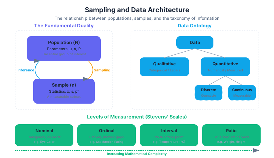
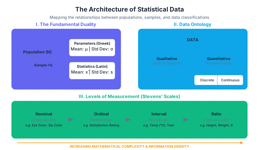
The Fundamental Duality: Population vs. Sample

In any statistical inquiry, we must first define the scope of our interest. This leads to the primary distinction in the field: the Population and the Sample.

The Population

The Population is the complete collection of all individuals, objects, or measurements whose properties are being studied. It is the "universe" of our investigation. In mathematical notation, the size of a finite population is often denoted by $N$.

Definition: A Population is the entire group that is the target of an investigation. It is the set of all possible observations of a specific phenomenon.

The Sample

In practice, measuring every member of a population is often impossible due to constraints of time, cost, or accessibility. Instead, we select a Sample—a subset of the population. The size of a sample is denoted by $n$. The goal of sampling is to obtain a representative group that mirrors the characteristics of the population, allowing us to perform inferential statistics.

Feature	Population	Sample
Definition	The entire group of interest.	A subset of the population.
Size Symbol	$N$	$n$
Accessibility	Often theoretical or inaccessible.	Tangible and measurable.
Goal	To understand the "true" state.	To estimate the population state.
Cost	Prohibitively high for large groups.	Manageable and optimized.

Parameters vs. Statistics

The distinction between population and sample necessitates a distinction in the values we calculate from them. We use different terminology and symbols to clarify whether we are describing the "truth" of the population or an "estimate" from the sample.

Parameters

A Parameter is a numerical characteristic of a whole population. Because the population is usually not fully observed, parameters are often unknown constants. We represent parameters using Greek letters.

Statistics

A Statistic is a numerical characteristic of a sample. Unlike parameters, statistics are known once the data is collected. However, because samples vary, a statistic is a random variable. We represent statistics using Latin letters.

Metric	Population Parameter (Greek)	Sample Statistic (Latin)
Mean (Average)	$\mu$ (mu)	$\bar{x}$ (x-bar)
Standard Deviation	$\sigma$ (sigma)	$s$
Proportion	$P$ or $\pi$ (pi)	$\hat{p}$ (p-hat)
Variance	$\sigma^2$	$s^2$

Key Insight: The central problem of statistics is Estimation. We use the sample statistic ($\bar{x}$) to make an educated guess about the population parameter ($\mu$). The difference between the two is known as the sampling error.

Data Ontology: Categorizing Information

Data is the raw material of statistics. To analyze it correctly, we must categorize it based on its mathematical properties. Not all data can be averaged, and not all data can be ranked.

Qualitative (Categorical) Data

Qualitative Data consists of attributes, labels, or non-numerical entries. These describe "qualities" rather than "quantities."

• Examples: Hair color, blood type, political affiliation, car make.
• Operations: We can count frequencies and calculate proportions, but we cannot calculate a "mean" hair color.

Quantitative (Numerical) Data

Quantitative Data consists of numbers that result from counting or measuring. These are further divided into two critical sub-types:

1. Discrete Data: Data that can only take on specific, "countable" values. There are gaps between values.
   • Example: The number of children in a family (you can't have 2.4 children).
2. Continuous Data: Data that can take on any value within a range. It is usually the result of a measurement.
   • Example: The weight of a person, the time spent waiting in line, the distance between cities.

Data Type	Sub-type	Description	Example
Qualitative	N/A	Labels or categories.	Type of OS (Linux, Windows, macOS)
Quantitative	Discrete	Countable integers.	Number of CPU cores
Quantitative	Continuous	Measurable, infinite precision.	Processor clock speed (GHz)

Levels of Measurement (Stevens' Scales)

Beyond the qualitative/quantitative split, we classify data into four levels of measurement. This hierarchy determines which statistical operations are mathematically valid.

1. Nominal Level: Data that is classified into categories with no inherent order.
   • Valid Ops: Mode, Frequency. (e.g., Zip codes, Gender).
2. Ordinal Level: Data that can be ordered or ranked, but the differences between values are meaningless.
   • Valid Ops: Median, Percentiles. (e.g., Movie ratings: 1-star, 2-star, 3-star).
3. Interval Level: Data with a defined ordering and measurable differences, but no true zero point.
   • Valid Ops: Addition, Subtraction, Mean. (e.g., Temperature in Celsius—0°C doesn't mean "no temperature").
4. Ratio Level: Data with an ordering, measurable differences, and a true zero point (where zero means "none").
   • Valid Ops: Multiplication, Division, Ratios. (e.g., Height, Weight, Salary).

Sampling Methodologies: The Mechanics of Collection

The validity of any statistical conclusion depends entirely on the quality of the sample. If a sample is not representative, it is biased, and the resulting statistics will systematically deviate from the true parameters.

1. Simple Random Sampling (SRS)

Every member of the population has an equal chance of being selected. This is the "gold standard" of sampling.

• Mechanism: Using a random number generator to pick $n$ individuals from a list of $N$.

2. Stratified Sampling

The population is divided into subgroups (strata) based on a specific characteristic (e.g., age, gender, income). A random sample is then taken from each stratum.

• Use Case: Ensuring that minority groups are adequately represented in the sample.

3. Cluster Sampling

The population is divided into groups (clusters), often geographically. A few clusters are selected at random, and all members within those selected clusters are sampled.

• Use Case: Large-scale surveys where it is too expensive to travel to every individual (e.g., sampling entire city blocks).

4. Systematic Sampling

Selecting every $k$-th individual from a list.

• Mechanism: Pick a random starting point between 1 and $k$, then select every $k$-th person thereafter.

5. Convenience Sampling

Selecting individuals who are easiest to reach.

• Warning: This method is highly prone to bias and is generally avoided in rigorous research.

Method	Strategy	Best Used When...	Risk
Simple Random	Pure chance.	The population is homogeneous.	High variance in small samples.
Stratified	Sample from every group.	You want to compare subgroups.	Requires knowing strata in advance.
Cluster	Sample entire groups.	Population is spread out geographically.	Clusters may not represent the whole.
Systematic	Every $k$-th person.	You have a stream of data (e.g., assembly line).	Hidden patterns in the list order.

Implementation: Sampling in Practice

To understand how these concepts manifest in technical environments, we look at how data is sampled in code, mathematics, and database systems.

Low-Level Implementation: Stratified Sampling in Python

In data science, we often need to ensure our training and testing sets maintain the same class proportions as the original dataset.

import numpy as np
import pandas as pd

def perform_stratified_sample(df, group_col, n_samples_per_group):
    """
    Manually implements stratified sampling to ensure equal representation.
    """
    # Group the dataframe by the target characteristic
    groups = df.groupby(group_col)
    
    # Sample n_samples from each group
    sampled_df = groups.apply(lambda x: x.sample(n=min(len(x), n_samples_per_group)))
    
    # Reset index to clean up the multi-index created by groupby
    return sampled_df.reset_index(drop=True)

# Example Usage:
# Create a dummy dataset of 1000 users with different 'Plan' types
data = {
    'user_id': range(1000),
    'plan': ['Free'] * 800 + ['Pro'] * 150 + ['Enterprise'] * 50
}
df = pd.DataFrame(data)

# We want 20 users from each plan to ensure we test Enterprise users properly
stratified_sample = perform_stratified_sample(df, 'plan', 20)
print(stratified_sample['plan'].value_counts())

Mathematical Representation: The Logic of Inference

The relationship between a sample statistic and a population parameter is governed by the Sampling Distribution. For a sample mean $\bar{x}$, the expected value is the population mean $\mu$, but the precision depends on the sample size $n$.

\text{Let } X_1, X_2, \dots, X_n \text{ be i.i.d. random variables from a population with mean } \mu \text{ and variance } \sigma^2.

\text{The Sample Mean is defined as: } 
\bar{x} = \frac{1}{n} \sum_{i=1}^{n} X_i

\text{The Expected Value of the Sample Mean is: }
E[\bar{x}] = E\left[\frac{1}{n} \sum X_i\right] = \frac{1}{n} \sum E[X_i] = \frac{1}{n} (n\mu) = \mu

\text{The Variance of the Sample Mean (Standard Error squared) is: }
Var(\bar{x}) = Var\left(\frac{1}{n} \sum X_i\right) = \frac{1}{n^2} \sum Var(X_i) = \frac{n\sigma^2}{n^2} = \frac{\sigma^2}{n}

Database Implementation: Random Sampling in SQL

When dealing with massive datasets (Big Data), we cannot load everything into memory. We use SQL's built-in sampling capabilities.

-- Method 1: Bernoulli Sampling (Randomly selects rows with a probability)
-- Useful for very large tables where you want roughly 1% of the data.
SELECT * 
FROM user_logs TABLESAMPLE BERNOULLI (1);

-- Method 2: Order By Random (Standard SQL, but slow on large tables)
-- This forces a full table scan and sort.
SELECT user_id, action_timestamp
FROM user_logs
ORDER BY RANDOM()
LIMIT 1000;

-- Method 3: Hash-based Sampling (Deterministic Sampling)
-- Useful for ensuring the same "random" sample is pulled every time.
SELECT *
FROM user_logs
WHERE MOD(ABS(HASH(user_id)), 100) < 5; -- Pulls a consistent 5% sample

Variation, Error, and Bias

Variation is natural; error is often structural. Understanding the difference is key to interpreting data.

Sampling Error

Even with a perfect random sampling method, the sample statistic will likely not equal the population parameter exactly. This discrepancy is Sampling Error. It is not a "mistake"—it is a natural consequence of using a subset to represent a whole. As $n$ increases, sampling error decreases.

Non-Sampling Error

These are errors caused by the data collection process itself. They do not disappear by increasing the sample size.

• Selection Bias: The sampling method systematically excludes certain segments of the population (e.g., an online survey excludes people without internet).
• Non-Response Bias: People who choose not to respond to a survey may have different opinions than those who do.
• Measurement Error: Poorly worded questions or faulty equipment lead to inaccurate data.

The Law of Large Numbers (LLN)

As the number of trials or the sample size increases, the sample mean $\bar{x}$ converges to the population mean $\mu$. This is the mathematical justification for why sampling works.

Common Pitfalls in Sampling

1. Confusing "Random" with "Haphazard": Standing on a street corner and talking to whoever walks by is not random sampling; it is convenience sampling. A true random sample requires a sampling frame (a list) where every member has a known, non-zero probability of selection.
2. Ignoring the "Small n" Problem: Small samples are highly susceptible to outliers. A single extreme value in a sample of 5 can swing the mean significantly, whereas it would be dampened in a sample of 500.
3. Self-Selection Bias: Allowing subjects to volunteer for a study (e.g., Yelp reviews) creates a sample of people with strong opinions, which rarely represents the "average" experience.
4. Treating Ordinal Data as Interval: Calculating the "average" of a Likert scale (1=Strongly Disagree, 5=Strongly Agree) is common but technically controversial, as the "distance" between "Neutral" and "Agree" may not be the same as the distance between "Agree" and "Strongly Agree."

Descriptive Statistics

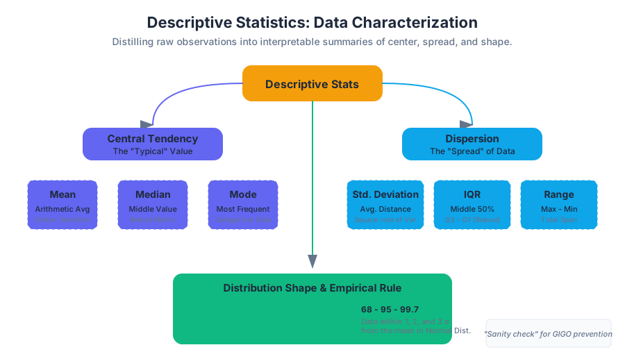
Descriptive statistics represents the foundational layer of data science and analytical reasoning. Rather than making inferences about a population from a sample, descriptive statistics focuses on the characterization and summarization of the data currently at hand. It is the process of data compression: taking a raw dataset—which may contain millions of individual observations—and distilling it into a few interpretable values and visualizations that capture its essence.

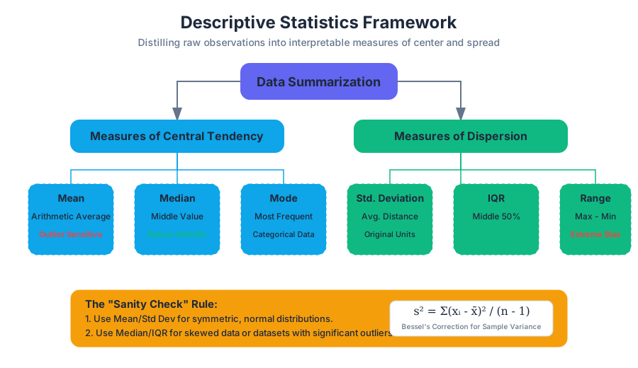
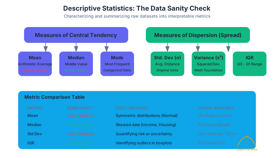
In the modern data pipeline, descriptive statistics serves as the "Sanity Check" phase. Before complex machine learning models are deployed or hypothesis tests are conducted, an analyst must understand the central tendency, the dispersion, and the shape of the data distribution. Without this, one risks the "Garbage In, Garbage Out" (GIGO) failure mode, where outliers or skewed distributions invalidate downstream logic.

Measures of Central Tendency

Central tendency refers to the "typical" or "middle" value of a dataset. While the concept seems intuitive, the choice of which measure to use depends heavily on the data's scale, distribution, and the presence of outliers.

The Mean (Arithmetic Average)

The Mean is the sum of all values divided by the number of observations. Mathematically, for a sample $x$, it is denoted as $\bar{x}$:

Definition: Arithmetic Mean $$\bar{x} = \frac{1}{n} \sum_{i=1}^{n} x_i$$ Where $n$ is the number of observations and $x_i$ represents each individual value.

The mean is the "balance point" of the data. However, it is highly sensitive to outliers. A single extreme value can pull the mean far away from the bulk of the data, making it a poor representation of "typicality" in skewed datasets (e.g., household income).

The Median

The Median is the middle value when the data is sorted in ascending or descending order. If the dataset has an even number of observations, the median is the average of the two central values.

The median is a robust statistic. Unlike the mean, it is resistant to outliers. In a dataset of $[10, 20, 30, 40, 1000]$, the mean is $220$, while the median is $30$. The median provides a better sense of the "typical" value in this context.

The Mode

The Mode is the value that appears most frequently in a dataset. A distribution can be unimodal (one mode), bimodal (two modes), or multimodal. It is the only measure of central tendency that can be used with nominal (categorical) data, such as "favorite color" or "operating system."

Metric	Sensitivity to Outliers	Data Type Suitability	Best Use Case
Mean	High	Interval, Ratio	Symmetric distributions (e.g., heights)
Median	Low (Robust)	Ordinal, Interval, Ratio	Skewed distributions (e.g., salaries)
Mode	Low	Nominal, Ordinal, Discrete	Categorical data (e.g., most popular product)

Implementation: Calculating Central Tendency

In high-performance data environments, we often use libraries like NumPy to handle these calculations efficiently over large arrays.

import numpy as np
from scipy import stats

def calculate_central_tendency(data):
    """
    Calculates Mean, Median, and Mode using NumPy and SciPy.
    Handles potential NaN values and multi-modal distributions.
    """
    # Remove NaNs for clean calculation
    clean_data = data[~np.isnan(data)]
    
    mean_val = np.mean(clean_data)
    median_val = np.median(clean_data)
    
    # SciPy's mode returns an object containing the mode(s) and their counts
    mode_res = stats.mode(clean_data, keepdims=True)
    mode_val = mode_res.mode[0]
    mode_count = mode_res.count[0]

    return {
        "mean": mean_val,
        "median": median_val,
        "mode": mode_val,
        "mode_frequency": mode_count
    }

# Example usage with a skewed dataset
dataset = np.array([12, 15, 12, 18, 20, 100, 12, 14, 15, np.nan])
stats_dict = calculate_central_tendency(dataset)
print(f"Results: {stats_dict}")

Measures of Dispersion (Spread)

Knowing the center of the data is insufficient. Two datasets can have the exact same mean but look entirely different. Dispersion describes how spread out the values are around the center.

Variance and Standard Deviation

The Variance ($\sigma^2$ for population, $s^2$ for sample) measures the average squared deviation from the mean. Because variance is in "squared units," we take its square root to get the Standard Deviation ($\sigma$ or $s$), which returns the measure to the original units of the data.

Theorem: Bessel's Correction When calculating the sample variance ($s^2$), we divide by $n-1$ instead of $n$. This corrects the bias in the estimation of the population variance, as a sample tends to underestimate the true spread of the population. $$s^2 = \frac{\sum (x_i - \bar{x})^2}{n - 1}$$

Range and Interquartile Range (IQR)

• Range: The difference between the maximum and minimum values. It is extremely sensitive to outliers.
• IQR: The difference between the 75th percentile ($Q_3$) and the 25th percentile ($Q_1$). It represents the spread of the middle 50% of the data and is a robust measure of dispersion.

The Empirical Rule (68-95-99.7)

For data that follows a Normal Distribution (bell curve):

• Approximately 68% of the data falls within $1\sigma$ of the mean.
• Approximately 95% falls within $2\sigma$.
• Approximately 99.7% falls within $3\sigma$.

Mathematical Derivation: Variance

The following pseudocode represents the mathematical steps required to derive the variance from scratch, emphasizing the importance of the sum of squares.

ALGORITHM CalculateSampleVariance(Dataset X):
    1.  n = length(X)
    2.  IF n < 2 THEN RETURN 0
    
    3.  Sum = 0
    4.  FOR EACH value x IN X:
            Sum = Sum + x
    5.  Mean = Sum / n
    
    6.  SumOfSquaredDeviations = 0
    7.  FOR EACH value x IN X:
            Deviation = x - Mean
            SquaredDeviation = Deviation * Deviation
            SumOfSquaredDeviations = SumOfSquaredDeviations + SquaredDeviation
            
    8.  Variance = SumOfSquaredDeviations / (n - 1)  // Applying Bessel's Correction
    9.  RETURN Variance

Graphical Displays: Visualizing the Distribution

Numerical summaries can be deceptive (see: Anscombe's Quartet). Visualization is essential to reveal the "shape" of the data.

Histograms

A Histogram groups continuous data into "bins" and displays the frequency of observations within each bin. It is the primary tool for identifying the shape of a distribution:

• Symmetric: The left and right sides are mirror images.
• Left-Skewed (Negative): The tail extends to the left; the mean is typically less than the median.
• Right-Skewed (Positive): The tail extends to the right; the mean is typically greater than the median.

Box Plots (Box-and-Whisker)

A Box Plot provides a visual summary of the "Five-Number Summary":

1. Minimum: The lowest data point (excluding outliers).
2. First Quartile ($Q_1$): The 25th percentile.
3. Median ($Q_2$): The 50th percentile.
4. Third Quartile ($Q_3$): The 75th percentile.
5. Maximum: The highest data point (excluding outliers).

Outliers in a box plot are typically defined using Tukey’s Fences: any point more than $1.5 \times IQR$ above $Q_3$ or below $Q_1$.

Feature	Histogram	Box Plot
Primary Goal	Show the shape/density of distribution.	Show quartiles, spread, and outliers.
Granularity	High (depends on bin size).	Low (summarizes into 5 points).
Outlier Detection	Visual gaps in bars.	Explicitly marked points.
Comparison	Hard to overlay many distributions.	Excellent for comparing multiple groups side-by-side.

Implementation: SQL for Descriptive Statistics

In many real-world scenarios, data is too large to pull into memory. We use SQL to calculate these descriptors directly within the database.

-- Calculating Descriptive Statistics for a 'sales' table in PostgreSQL
SELECT 
    COUNT(price) AS sample_size,
    AVG(price) AS mean_price,
    PERCENTILE_CONT(0.5) WITHIN GROUP (ORDER BY price) AS median_price,
    MIN(price) AS min_price,
    MAX(price) AS max_price,
    MAX(price) - MIN(price) AS range,
    STDDEV(price) AS std_dev,
    VARIANCE(price) AS sample_variance,
    -- Calculating IQR
    PERCENTILE_CONT(0.75) WITHIN GROUP (ORDER BY price) - 
    PERCENTILE_CONT(0.25) WITHIN GROUP (ORDER BY price) AS iqr
FROM 
    ecommerce.transactions
WHERE 
    transaction_date >= '2023-01-01';

Advanced Concepts: Skewness and Kurtosis

Beyond center and spread, we describe the "style" of the distribution's shape.

Skewness

Skewness measures the asymmetry of the probability distribution.

• A skewness of 0 indicates perfect symmetry.
• Positive skew indicates a long right tail (common in wealth distribution).
• Negative skew indicates a long left tail (common in age of retirement).

Kurtosis

Kurtosis measures the "tailedness" of the distribution.

• Mesokurtic: Similar to a normal distribution (Kurtosis $\approx 3$).
• Leptokurtic: Heavy tails and a sharp peak (indicates frequent extreme outliers).
• Platykurtic: Thin tails and a flat peak (indicates fewer outliers than a normal distribution).

Common Pitfalls in Descriptive Statistics

1. Over-reliance on the Mean: Using the mean for highly skewed data (like startup valuations) leads to a distorted view of reality. Always check the median.
2. Binning Bias in Histograms: Choosing bins that are too wide hides patterns; choosing bins that are too narrow creates noise. Use the Freedman-Diaconis rule for optimal bin width: $h = 2 \frac{IQR(x)}{\sqrt[3]{n}}$.
3. Ignoring the Sample Size: A standard deviation of 10 means something very different if $n=5$ versus $n=5000$.
4. Confusing Standard Deviation with Standard Error: Standard deviation describes the spread of the data, while standard error describes the uncertainty of the mean estimate.

Practical Example: Analyzing Server Latency

Imagine you are a Site Reliability Engineer (SRE) monitoring API response times.

• Mean Latency: 200ms.
• Median Latency: 150ms.
• 99th Percentile (P99): 2500ms.

If you only looked at the mean, you might think the system is performing well. However, the gap between the median (150ms) and the mean (200ms) suggests a right-skewed distribution. The P99 of 2500ms reveals that while most users have a fast experience, 1% of users are experiencing a 2.5-second delay—a critical issue that the mean obscures.

Summary Table: Choosing the Right Statistic

Scenario	Recommended Measure	Why?
Reporting average salaries	Median	Prevents high-earning outliers from inflating the "average."
Manufacturing quality control	Standard Deviation	Measures consistency; lower is better.
Analyzing website traffic spikes	Mode	Identifies the most common time of day users visit.
Comparing test scores across classes	Box Plot	Shows the spread and identifies struggling/excelling students easily.
Determining "normal" heart rate	Mean + Std Dev	Heart rate is generally normally distributed in healthy populations.

Probability Topics

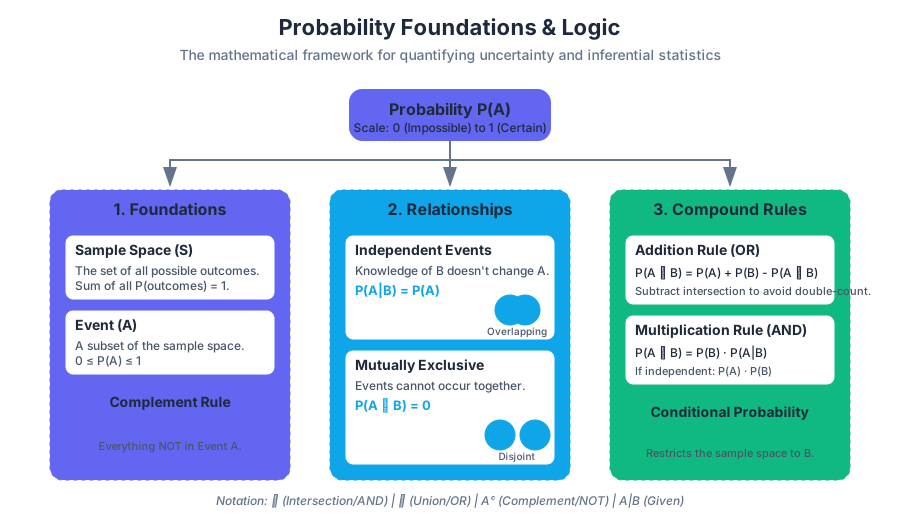
Probability is the mathematical language of uncertainty. While descriptive statistics allows us to summarize the past, probability provides the theoretical framework required for inferential statistics—the process of using sample data to make assertions about a population. In technical terms, probability is a measure of the likelihood that an event will occur, mapped onto a scale from 0 (impossibility) to 1 (certainty).

The Foundations: Sample Spaces and Events

To analyze any probabilistic system, we must first define the Sample Space ($S$), which is the set of all possible outcomes. An Event is any subset of that sample space. The probability of an event $A$, denoted $P(A)$, is the sum of the probabilities of the individual outcomes within that event.

The Axioms of Probability:

1. For any event $A$, $0 \le P(A) \le 1$.
2. The sum of probabilities of all possible outcomes in $S$ is exactly 1.
3. The probability of an event occurring is the sum of the probabilities of the outcomes that comprise it.

The Complement Rule

The Complement of an event $A$ (denoted as $A'$ or $A^c$) consists of all outcomes in the sample space that are not in $A$. The Complement Rule is one of the most powerful shortcuts in probability, particularly when calculating "at least one" scenarios.

$$P(A) + P(A^c) = 1 \implies P(A^c) = 1 - P(A)$$

Concept	Notation	Definition	Logical Equivalent
Event	$A$	A specific outcome or set of outcomes.	"It happens."
Complement	$A^c$	All outcomes in $S$ not in $A$.	"It does not happen."
Intersection	$A \cap B$	Outcomes common to both $A$ and $B$.	"Both $A$ AND $B$."
Union	$A \cup B$	Outcomes in $A$, $B$, or both.	"Either $A$ OR $B$."

---

Conditional Probability: The Logic of Updated Information

Conditional Probability is the probability that event $A$ occurs, given that event $B$ has already occurred. This is written as $P(A|B)$, read as "the probability of $A$ given $B$."

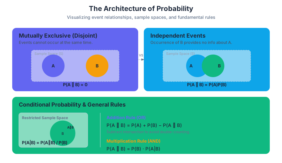
Mathematically, conditional probability effectively restricts the sample space. Instead of looking at the entire universe of possibilities $S$, we ignore everything outside of $B$.

The Formula

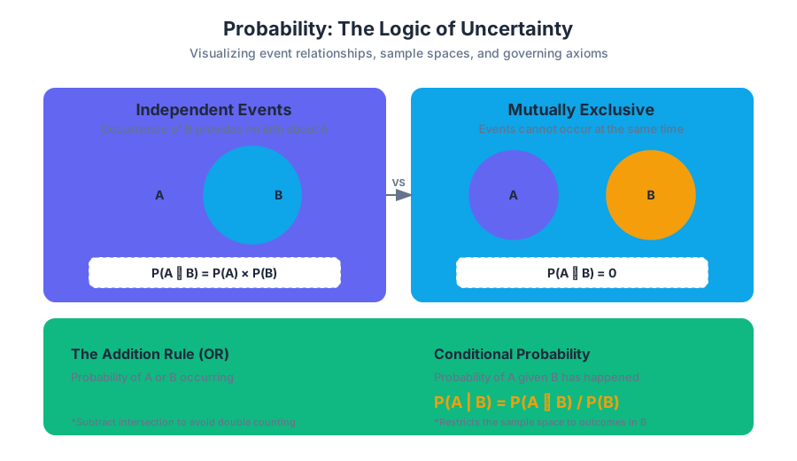
$$P(A|B) = \frac{P(A \cap B)}{P(B)}$$ Note: This is only defined if $P(B) > 0$.

Why It Matters

Conditional probability is the engine behind Bayesian inference, spam filters, and medical diagnostics. It allows us to update our beliefs as new data arrives. For example, the probability that a person has a specific disease ($A$) changes significantly once we know they have tested positive ($B$).

# Python Implementation: Calculating Conditional Probability from Raw Event Data
import numpy as np

def calculate_conditional_probability(event_a_mask, event_b_mask):
    """
    Calculates P(A|B) given boolean masks of occurrences.
    """
    # P(B)
    prob_b = np.mean(event_b_mask)
    
    if prob_b == 0:
        return 0.0  # Avoid division by zero
    
    # P(A and B)
    prob_a_and_b = np.mean(event_a_mask & event_b_mask)
    
    # P(A|B) = P(A and B) / P(B)
    return prob_a_and_b / prob_b

# Example: 10,000 trials of rolling two dice
dice_1 = np.random.randint(1, 7, 10000)
dice_2 = np.random.randint(1, 7, 10000)

# Event B: Sum is greater than 8
event_b = (dice_1 + dice_2) > 8
# Event A: Dice 1 is a 6
event_a = (dice_1 == 6)

p_a_given_b = calculate_conditional_probability(event_a, event_b)
print(f"Empirical P(Dice1=6 | Sum > 8): {p_a_given_b:.4f}")

---

Independent Events vs. Mutually Exclusive Events

One of the most common points of confusion in statistics is the distinction between Independence and Mutual Exclusivity. While both describe relationships between events, they represent fundamentally different structural properties.

Independent Events

Two events $A$ and $B$ are Independent if the occurrence of one does not change the probability of the other. In other words, knowing that $B$ happened provides zero information about whether $A$ will happen.

Formal Tests for Independence: Two events are independent if and only if:

1. $P(A|B) = P(A)$
2. $P(B|A) = P(B)$
3. $P(A \cap B) = P(A) \cdot P(B)$

Mutually Exclusive (Disjoint) Events

Two events are Mutually Exclusive if they cannot happen at the same time. If $A$ happens, $B$ cannot happen. Their intersection is an empty set.

Formal Test for Mutual Exclusivity: $$P(A \cap B) = 0$$

Comparison Table

Feature	Independent Events	Mutually Exclusive Events
Definition	One event doesn't affect the other's likelihood.	The events cannot occur simultaneously.
Intersection	$P(A \cap B) = P(A)P(B)$	$P(A \cap B) = 0$
Relationship	Information-based (Knowledge of $B$ is useless).	Occurrence-based (Occurrence of $B$ precludes $A$).
Can they be both?	No (unless one event has probability 0).	No.
Visual Representation	Overlapping areas in a Venn diagram.	Non-overlapping circles in a Venn diagram.

---

The Multiplication and Addition Rules

These rules allow us to combine probabilities to find the likelihood of complex compound events.

1. The Multiplication Rule (The "AND" Rule)

Used to find the probability of the intersection $P(A \cap B)$.

• General Rule: $P(A \cap B) = P(B) \cdot P(A|B)$
• If Independent: $P(A \cap B) = P(A) \cdot P(B)$

2. The Addition Rule (The "OR" Rule)

Used to find the probability of the union $P(A \cup B)$.

• General Rule: $P(A \cup B) = P(A) + P(B) - P(A \cap B)$
• If Mutually Exclusive: $P(A \cup B) = P(A) + P(B)$

Mathematical Derivation of the General Addition Rule

The subtraction of $P(A \cap B)$ is necessary because the intersection is counted twice—once in $P(A)$ and once in $P(B)$.

\begin{aligned}
\text{Let } S &= \text{Sample Space} \\
P(A \cup B) &= \frac{|A \cup B|}{|S|} \\
\text{By Principle of Inclusion-Exclusion:} \\
|A \cup B| &= |A| + |B| - |A \cap B| \\
\implies \frac{|A \cup B|}{|S|} &= \frac{|A|}{|S|} + \frac{|B|}{|S|} - \frac{|A \cap B|}{|S|} \\
P(A \cup B) &= P(A) + P(B) - P(A \cap B)
\end{aligned}

---

Tools for Visualization and Calculation

When dealing with multiple events, raw formulas can become cumbersome. Professional statisticians use three primary tools to organize their logic.

1. Contingency Tables (Two-Way Tables)

These are ideal for analyzing the relationship between two categorical variables. They allow for easy calculation of marginal, joint, and conditional probabilities.

Example: Product Defects by Shift

	Defective (D)	Non-Defective (N)	Total
Day Shift (S1)	15	485	500
Night Shift (S2)	25	475	500
Total	40	960	1000

From this table:

• $P(D) = 40/1000 = 0.04$
• $P(D|S2) = 25/500 = 0.05$
• Since $P(D|S2) \neq P(D)$, the shift and defect rate are not independent.

2. Tree Diagrams

Tree diagrams are best for sequential events or multi-stage experiments where the outcome of the first stage affects the probabilities of the second.

3. Venn Diagrams

Venn diagrams are the gold standard for visualizing the logical relationship (unions and intersections) between 2 or 3 events.

---

Practical Application: Data Analysis and SQL

In a modern data stack, probability calculations are often performed directly in the database to filter segments or calculate risk scores.

-- Calculating Conditional Probability in SQL
-- Question: What is the probability of a 'Churn' event (A) 
-- given the customer had a 'Support Ticket' (B)?

WITH EventCounts AS (
    SELECT 
        COUNT(*) AS total_customers,
        SUM(CASE WHEN has_support_ticket = 1 THEN 1 ELSE 0 END) AS count_b,
        SUM(CASE WHEN has_support_ticket = 1 AND has_churned = 1 THEN 1 ELSE 0 END) AS count_a_and_b
    FROM customers_table
)
SELECT 
    -- P(B)
    CAST(count_b AS FLOAT) / total_customers AS prob_support_ticket,
    
    -- P(A and B)
    CAST(count_a_and_b AS FLOAT) / total_customers AS prob_churn_and_ticket,
    
    -- P(A|B) = P(A and B) / P(B)
    CASE 
        WHEN count_b > 0 THEN CAST(count_a_and_b AS FLOAT) / count_b 
        ELSE 0 
    END AS conditional_prob_churn_given_ticket
FROM EventCounts;

---

Common Pitfalls and Misconceptions

The Gambler’s Fallacy

The mistaken belief that if an event happens more frequently than normal during a given period, it will happen less frequently in the future (or vice versa). This is a failure to recognize Independence. If you flip a fair coin 10 times and get 10 heads, the probability of tails on the 11th flip is still exactly 0.5.

Confusing "Independent" with "Mutually Exclusive"

As noted in the comparison table, these are nearly opposites. If two events are mutually exclusive (and have non-zero probability), they cannot be independent. Why? Because if $A$ occurs, the probability of $B$ immediately drops to 0. The occurrence of $A$ gave you perfect information about $B$, which is the definition of dependence.

The Base Rate Fallacy

Ignoring the overall probability of an event (the "base rate") when presented with specific evidence. This is a common error in medical testing interpretation, where people focus on the test's accuracy but ignore how rare the disease is in the general population.

---

Summary of Formulas

Rule	Formula	Context
Complement	$P(A^c) = 1 - P(A)$	Finding "not A"
Addition (General)	$P(A \cup B) = P(A) + P(B) - P(A \cap B)$	Finding "A or B"
Addition (M.E.)	$P(A \cup B) = P(A) + P(B)$	Finding "A or B" when they can't overlap
Multiplication (General)	$P(A \cap B) = P(B) \cdot P(A\vert B)$	Finding "A and B"
Multiplication (Indep.)	$P(A \cap B) = P(A) \cdot P(B)$	Finding "A and B" when they don't affect each other
Conditional	$P(A\vert B) = \frac{P(A \cap B)}{P(B)}$	Finding "A given B"

Discrete Random Variables

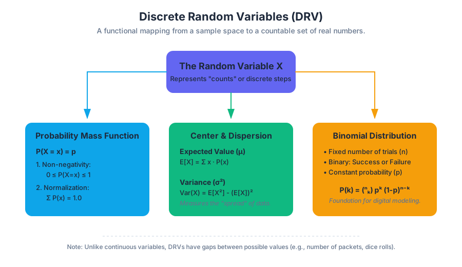
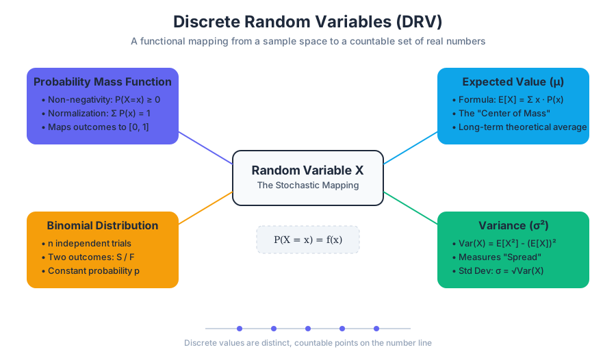
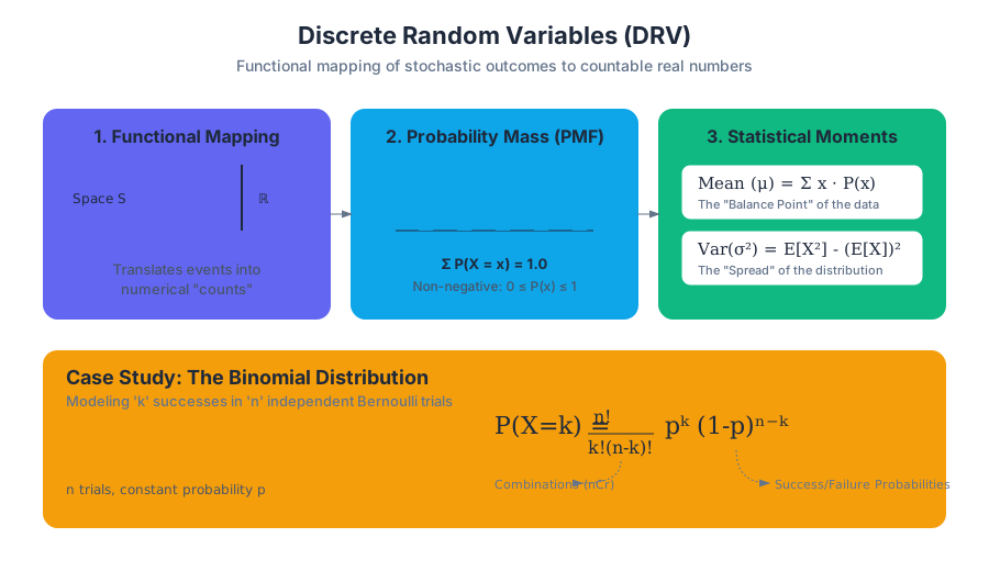
In the study of probability and statistics, a Random Variable serves as a functional mapping from the sample space of a stochastic process to the set of real numbers. When the set of possible outcomes is countable—meaning the values can be listed as a finite sequence or an infinite sequence like the integers—we define this as a Discrete Random Variable (DRV).

Unlike continuous variables, which represent measurements along a continuum (like height or time), discrete variables represent "counts." They are the fundamental building blocks for modeling digital systems, queuing theory, and categorical data analysis. Whether quantifying the number of defective microchips in a production batch or the number of packets arriving at a network router, DRVs provide the mathematical framework for predicting long-term behavior in uncertain environments.

The Probability Distribution Function (PDF)

For a discrete random variable $X$, the Probability Distribution Function (PDF)—often more precisely called the Probability Mass Function (PMF) in discrete contexts—is a mathematical description of the probabilities associated with each possible value of $X$.

1. What it is

The PDF, denoted as $P(X = x)$ or $f(x)$, maps each outcome $x$ in the support of the distribution to a probability $p$. For a function to qualify as a valid PDF for a discrete random variable, it must satisfy two rigorous conditions:

1. Non-negativity: $0 \le P(X = x) \le 1$ for all $x$.
2. Normalization: The sum of all probabilities over the entire sample space must equal exactly one: $\sum P(x) = 1$.

2. Why it matters

The PDF is the "DNA" of the random variable. It allows us to calculate not just the likelihood of a single event, but the likelihood of ranges (e.g., "What is the probability of having at least 3 successes?"). Without a well-defined PDF, we cannot derive the moments of the distribution, such as the mean or variance.

3. Formal Properties and Structure

The relationship between the variable and its probability is often represented in a distribution table.

Outcome ($x$)	Probability $P(X=x)$	Cumulative Probability $P(X \le x)$
$x_1$	$p_1$	$p_1$
$x_2$	$p_2$	$p_1 + p_2$
$x_n$	$p_n$	$1.0$

4. Implementation Example: Building a Discrete Distribution

In computational environments, we often represent a PDF as a mapping or a normalized frequency array.

import numpy as np

class DiscreteDistribution:
    """
    A low-level implementation of a Discrete Random Variable PDF.
    Handles validation and basic statistical queries.
    """
    def __init__(self, outcomes, probabilities):
        self.outcomes = np.array(outcomes)
        self.probabilities = np.array(probabilities)
        
        # Validation: Probabilities must sum to 1 (within floating point error)
        if not np.isclose(np.sum(self.probabilities), 1.0):
            raise ValueError("Probabilities must sum to 1.0")
        
        # Validation: No negative probabilities
        if np.any(self.probabilities < 0):
            raise ValueError("Probabilities cannot be negative")

    def pmf(self, x):
        """Returns P(X = x)"""
        idx = np.where(self.outcomes == x)[0]
        return self.probabilities[idx[0]] if idx.size > 0 else 0.0

    def cdf(self, x):
        """Returns P(X <= x) - The Cumulative Distribution Function"""
        return np.sum(self.probabilities[self.outcomes <= x])

# Example: A biased 4-sided die
outcomes = [1, 2, 3, 4]
probs = [0.1, 0.2, 0.4, 0.3]
die_dist = DiscreteDistribution(outcomes, probs)
print(f"P(X=3): {die_dist.pmf(3)}")
print(f"P(X<=2): {die_dist.cdf(2)}")

Expected Value and Variance

The Expected Value ($E[X]$ or $\mu$) represents the theoretical long-term average of a discrete random variable if the experiment were repeated an infinite number of times. It is the "center of mass" of the distribution.

1. Mechanics of Calculation

The expected value is a weighted average where each outcome is weighted by its probability:

Definition: $E[X] = \mu = \sum_{i} x_i P(x_i)$

While the expected value provides the location of the distribution, the Variance ($\sigma^2$) measures its spread—how much the outcomes typically deviate from the mean.

Definition: $Var(X) = \sigma^2 = \sum_{i} (x_i - \mu)^2 P(x_i)$

2. Comparison of Central Tendency and Dispersion

It is a common pitfall to assume the expected value must be one of the possible outcomes of the variable. For instance, the expected value of a fair six-sided die is 3.5, a value that is impossible to actually roll.

Metric	Formula	Interpretation
Mean ($\mu$)	$\sum x P(x)$	The "balance point" of the distribution.
Variance ($\sigma^2$)	$E[X^2] - (E[X])^2$	The average squared distance from the mean.
Std Dev ($\sigma$)	$\sqrt{Var(X)}$	Dispersion expressed in the same units as $X$.

3. Mathematical Derivation

The relationship between the raw moments and the variance is a critical identity in statistics.

\begin{aligned}
\text{Let } \mu &= E[X] \\
Var(X) &= E[(X - \mu)^2] \\
&= E[X^2 - 2X\mu + \mu^2] \\
&= E[X^2] - 2\mu E[X] + \mu^2 \\
&= E[X^2] - 2\mu^2 + \mu^2 \\
&= E[X^2] - (E[X])^2
\end{aligned}

The Binomial Distribution

The Binomial Distribution is the most widely used discrete distribution for modeling a fixed number of independent "success/failure" trials. It is the foundation of quality control, A/B testing in software engineering, and clinical trial analysis.

1. What it is: The Bernoulli Trial

A Binomial experiment consists of $n$ identical trials, known as Bernoulli Trials, which meet four specific criteria:

1. There are a fixed number of trials ($n$).
2. There are only two possible outcomes (Success or Failure).
3. The probability of success ($p$) is constant for every trial.
4. The trials are independent (the outcome of one does not affect the next).

2. The Probability Mass Function

The probability of achieving exactly $k$ successes in $n$ trials is given by:

$P(X = k) = \binom{n}{k} p^k q^{n-k}$ Where $q = 1 - p$ and $\binom{n}{k} = \frac{n!}{k!(n-k)!}$

3. Parameters and Characteristics

The behavior of a Binomial distribution is entirely determined by $n$ and $p$.

Parameter	Symbol	Effect on Distribution
Trials	$n$	Increases the range of possible outcomes; as $n \to \infty$, the distribution approaches Normal.
Success Prob	$p$	Determines skewness; $p=0.5$ is perfectly symmetric.
Mean	$\mu = np$	The average number of successes.
Variance	$\sigma^2 = npq$	The spread of successes.

4. Real-World Usage Example

Consider a DevOps scenario: A microservice has a 99% success rate ($p=0.99$). If 100 requests are sent, what is the probability that exactly 2 fail? This is a Binomial problem where $n=100$, $k=98$ (successes), and $p=0.99$.

from scipy.stats import binom

# Parameters
n = 100  # total requests
p = 0.99 # success probability
k = 98   # desired successes (2 failures)

# Calculate exact probability P(X = 98)
prob_exact = binom.pmf(k, n, p)

# Calculate cumulative probability P(X <= 95) - probability of more than 4 failures
prob_at_most_95 = binom.cdf(95, n, p)

print(f"Probability of exactly 98 successes: {prob_exact:.4f}")
print(f"Probability of 5 or more failures: {prob_at_most_95:.4f}")

The Poisson Distribution

While the Binomial distribution counts successes in a fixed number of trials, the Poisson Distribution models the number of events occurring within a fixed interval of time or space.

1. What it is

The Poisson distribution is used when events occur independently at a constant average rate. It is often referred to as the "Law of Rare Events." Examples include the number of emails received per hour, the number of typos per page, or the number of radioactive decays per second.

2. The Poisson PMF

The probability of observing $k$ events in an interval is:

$P(X = k) = \frac{\lambda^k e^{-\lambda}}{k!}$ Where $\lambda$ (lambda) is the average number of events in the given interval.

3. Key Properties

A unique property of the Poisson distribution is that its mean is equal to its variance:

• $E[X] = \lambda$
• $Var(X) = \lambda$

This makes the Poisson distribution highly restrictive but mathematically elegant for modeling arrival processes (Poisson Processes).

4. Poisson vs. Binomial: The Approximation

The Poisson distribution can be viewed as the limiting case of the Binomial distribution as $n \to \infty$ and $p \to 0$, while the product $np = \lambda$ remains constant. In practice, if $n \ge 100$ and $np \le 10$, the Poisson distribution is an excellent approximation for the Binomial.

Feature	Binomial Distribution	Poisson Distribution
Nature of Trials	Fixed number of trials ($n$)	Continuous interval (time/space)
Outcomes	Binary (Success/Failure)	Discrete counts (0, 1, 2, ...)
Upper Bound	$n$	Theoretically infinite
Parameters	$n, p$	$\lambda$

5. Common Pitfalls in Poisson Modeling

• Non-constant rate: If the rate of arrival changes (e.g., more customers at lunch than at 3 PM), a simple Poisson model fails. This requires a Non-Homogeneous Poisson Process.
• Clumping: Poisson assumes events are independent. If events occur in clusters (like "bursty" network traffic), the variance will exceed the mean (Overdispersion), and a Negative Binomial distribution may be more appropriate.

Practical Application: Choosing the Right Distribution

Selecting the correct distribution is the most critical step in statistical modeling. The following pipeline represents the decision matrix used by data scientists.

Decision Flow:

1. Is the data discrete? (Counts of items/events)
   • If No $\to$ Continuous (Normal, Exponential, etc.)
2. Is there a fixed number of trials ($n$)?
   • If Yes $\to$ Binomial (e.g., "Out of 20 tosses...")
3. Are we looking for the first success?
   • If Yes $\to$ Geometric (e.g., "How many tries until...")
4. Is the interval fixed (time/area) rather than trials?
   • If Yes $\to$ Poisson (e.g., "Hits per minute...")

Comparative Summary Table

Scenario	Distribution	Key Formula	Parameters
Binary outcomes, fixed trials	Binomial	$\binom{n}{k} p^k q^{n-k}$	$n, p$
Events in time/space interval	Poisson	$\frac{\lambda^k e^{-\lambda}}{k!}$	$\lambda$
Trials until first success	Geometric	$p(1-p)^{k-1}$	$p$
Sampling without replacement	Hypergeometric	$\frac{\binom{r}{k}\binom{N-r}{n-k}}{\binom{N}{n}}$	$N, r, n$

Advanced Concept: The Moment Generating Function (MGF)

For senior engineers and statisticians, defining a DRV by its PMF is often less efficient than using its Moment Generating Function. The MGF is a functional representation that encapsulates all moments (mean, variance, skewness, etc.) of a distribution.

M_X(t) = E[e^{tX}] = \sum_{x} e^{tx} P(X=x)

By taking the $n$-th derivative of $M_X(t)$ and evaluating it at $t=0$, one can derive the $n$-th raw moment of the variable. This is particularly useful when summing independent random variables, as the MGF of the sum is simply the product of the individual MGFs.

Continuous Random Variables

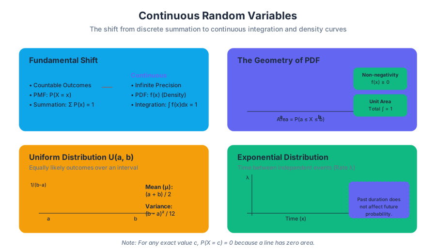
In the study of probability and statistics, we distinguish between two fundamental types of data: discrete and continuous. While discrete random variables deal with "countable" outcomes—the number of heads in a coin toss or the number of students in a classroom—continuous random variables represent measurements on a continuum. These variables can take on any value within a given range, often involving decimals or fractions of infinite precision.

From the perspective of a data scientist or engineer, the shift from discrete to continuous is a shift from summation to integration. We no longer ask for the probability that a variable equals a specific value; instead, we measure the probability that a variable falls within a specific interval. This distinction is the bedrock of modern statistical modeling, from predicting the lifespan of server hardware to modeling the latency of a microservice.

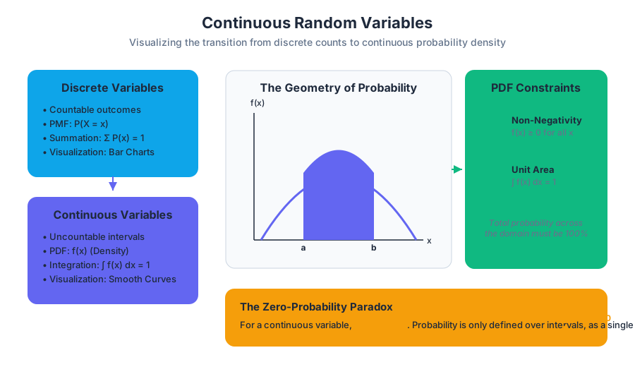
The Geometry of Probability: Density Curves

The behavior of a continuous random variable is described by a Probability Density Function (PDF), denoted as $f(x)$. Unlike discrete probability mass functions, the value of $f(x)$ at any specific point does not represent a probability. Instead, it represents the "density" of probability at that point.

The Fundamental Constraints

For a function to qualify as a valid PDF for a continuous random variable $X$, it must satisfy two rigorous mathematical conditions:

1. Non-negativity: $f(x) \ge 0$ for all possible values of $x$. Probability density cannot be negative.
2. Unit Area: The total area under the curve across the entire domain of $X$ must equal exactly 1. Mathematically: $\int_{-\infty}^{\infty} f(x) dx = 1$.

Area Under the Curve (AUC)

In the continuous domain, the probability that $X$ falls between two values $a$ and $b$ is defined as the area under the PDF curve between those two points.

The Zero-Probability Paradox: For any continuous random variable, the probability that $X$ is exactly equal to a specific value $c$ is zero ($P(X = c) = 0$). This is because the area of a line segment with width zero is zero. Consequently, $P(a \le X \le b)$ is identical to $P(a < X < b)$.

Feature	Discrete Random Variables	Continuous Random Variables
Values	Countable (integers, finite sets)	Uncountable (intervals, real numbers)
Function Type	Probability Mass Function (PMF)	Probability Density Function (PDF)
Probability at a point	$P(X=x) = f(x)$	$P(X=x) = 0$
Total Sum/Integral	$\sum P(x) = 1$	$\int f(x) dx = 1$
Visualization	Histograms / Bar Charts	Smooth Curves (Density Plots)

The Uniform Distribution

The Uniform Distribution is the simplest continuous distribution, often referred to as the "rectangular distribution." It models a scenario where every interval of the same length within the distribution's domain is equally likely.

Mathematical Definition

A continuous random variable $X$ follows a uniform distribution between $a$ and $b$, denoted as $X \sim U(a, b)$, if its PDF is:

$$f(x) = \begin{cases} \frac{1}{b - a} & \text{for } a \le x \le b \ 0 & \text{otherwise} \end{cases}$$

Key Parameters and Statistics

The uniform distribution is defined by its boundaries $a$ (minimum) and $b$ (maximum).

Statistic	Formula	Description
Mean ($\mu$)	$\frac{a + b}{2}$	The midpoint of the interval.
Variance ($\sigma^2$)	$\frac{(b - a)^2}{12}$	Measures the spread relative to the interval width.
Standard Deviation ($\sigma$)	$\sqrt{\frac{(b - a)^2}{12}}$	The square root of the variance.
CDF $F(x)$	$\frac{x - a}{b - a}$	The cumulative probability from $a$ to $x$.

Implementation: Generating Uniform Samples

In software engineering, uniform distributions are the "primitive" from which all other distributions are derived via the Inverse Transform Sampling method.

import numpy as np
import matplotlib.pyplot as plt

def generate_uniform_metrics(a, b, samples=10000):
    """
    Simulates a uniform distribution for a process, 
    such as the wait time for a bus that arrives every (b-a) minutes.
    """
    # Low-level implementation using NumPy's vectorized operations
    data = np.random.uniform(a, b, samples)
    
    # Calculate theoretical mean and variance
    theoretical_mean = (a + b) / 2
    theoretical_var = ((b - a)**2) / 12
    
    print(f"Empirical Mean: {np.mean(data):.4f} (Theoretical: {theoretical_mean})")
    print(f"Empirical Var:  {np.var(data):.4f} (Theoretical: {theoretical_var:.4f})")
    
    return data

# Usage: Bus arrives between 0 and 15 minutes
bus_wait_times = generate_uniform_metrics(0, 15)

The Exponential Distribution

While the Uniform distribution deals with "where," the Exponential Distribution is primarily concerned with "when." It is frequently used to model the time elapsed between independent events occurring at a constant average rate. Common applications include the time between radioactive decays, the time until a lightbulb fails, or the time between customer arrivals in a queue.

The Rate Parameter ($\lambda$)

The distribution is characterized by the rate parameter $\lambda$ (lambda), which represents the average number of events per unit of time. If a system receives 10 requests per second, $\lambda = 10$.

Probability Density Function

The PDF of an exponential distribution is defined for $x \ge 0$:

$$f(x) = \lambda e^{-\lambda x}$$

The Memoryless Property

Perhaps the most counter-intuitive and significant feature of the exponential distribution is that it is memoryless.

Definition: A random variable $X$ is memoryless if $P(X > s + t \mid X > s) = P(X > t)$ for all $s, t \ge 0$.

In practical terms, if the lifespan of a component is exponentially distributed, the probability that it will last another 100 hours is the same whether it is brand new or has already been running for 500 hours. The component does not "age" in a way that affects its immediate probability of failure.

Derivation of the Cumulative Distribution Function (CDF)

To find the probability that an event occurs within a certain time $x$, we integrate the PDF.

% Mathematical Derivation of the Exponential CDF
F(x) = P(X \le x) = \int_{0}^{x} \lambda e^{-\lambda t} dt
% Applying the fundamental theorem of calculus:
F(x) = [ -e^{-\lambda t} ]_{0}^{x}
F(x) = (-e^{-\lambda x}) - (-e^{0})
F(x) = 1 - e^{-\lambda x}

Comparison: Exponential vs. Poisson

It is vital to distinguish between the Poisson and Exponential distributions, as they are two sides of the same coin.

Distribution	Type	What it Measures	Parameter
Poisson	Discrete	The number of events in a fixed interval.	$\mu$ or $\lambda$ (Mean count)
Exponential	Continuous	The time between those events.	$\lambda$ (Rate) or $m = 1/\lambda$ (Mean time)

Practical Application: Reliability Engineering

In systems engineering, we often use the exponential distribution to model the Mean Time Between Failures (MTBF). If a hard drive has an MTBF of 500,000 hours, the rate $\lambda$ is $1/500,000$.

Real-World Usage Example: System Latency Analysis

Engineers often use CLI tools or scripts to validate if their system's latency follows an exponential decay, which would suggest random, independent request arrivals.

# Example: Using a shell pipeline to analyze request inter-arrival times
# 1. Extract timestamps from a log file
# 2. Calculate the difference between consecutive timestamps
# 3. Use 'awk' to calculate the mean (1/lambda)

cat access.log | \
awk '{print $1}' | \
perl -ne 'BEGIN{$last=0} $diff=$_-$last; print "$diff\n" if $last!=0; $last=$_' | \
awk '{sum+=$1; count++} END {if (count > 0) print "Mean Inter-arrival Time (1/lambda): " sum/count}'

Cumulative Distribution Functions (CDF) and Percentiles

The Cumulative Distribution Function (CDF), $F(x)$, is the probability that the random variable $X$ is less than or equal to $x$. For continuous variables, the CDF is the running integral of the PDF.

Calculating Percentiles

The $k$-th percentile is the value $x$ such that $P(X < x) = k/100$.

• For the Uniform Distribution, the median (50th percentile) is simply the mean $\frac{a+b}{2}$.
• For the Exponential Distribution, the median is $\frac{\ln(2)}{\lambda}$, which is approximately $0.693 \times \text{mean}$. Note that for exponential distributions, the median is always smaller than the mean due to the long right tail.

Summary of CDFs

Distribution	CDF Formula $F(x)$	Solving for $x$ (Percentile)
Uniform	$\frac{x-a}{b-a}$	$x = a + p(b-a)$
Exponential	$1 - e^{-\lambda x}$	$x = \frac{-\ln(1-p)}{\lambda}$

Common Pitfalls and Misconceptions

1. Confusing $f(x)$ with $P(X=x)$

In a continuous distribution, $f(x)$ can be greater than 1. For example, in $U(0, 0.5)$, the density $f(x) = 1/(0.5 - 0) = 2$. This is not a probability; the probability is the area, which will never exceed 1.

2. The Memoryless Property Misapplication

The memoryless property only applies to the Exponential distribution. It does not apply to the Normal distribution, nor does it apply to human aging or mechanical wear-and-tear that involves physical degradation (which usually follows a Weibull distribution).

3. Endpoint Inclusion

Beginners often worry whether to use $P(X < x)$ or $P(X \le x)$. In continuous probability, the boundary point has zero width and zero probability, so the choice of inequality ($<$ vs $\le$) is mathematically irrelevant.

4. The "Average" Trap

In skewed distributions like the Exponential, the "average" (mean) is not the "typical" (median) value. If the mean time to failure is 100 days, more than 50% of units will likely fail before 100 days because the mean is pulled higher by a few long-lasting outliers.

Advanced Extensions: The Relationship to the Normal Distribution

While Uniform and Exponential distributions are foundational, they often serve as building blocks for the Normal (Gaussian) Distribution. According to the Central Limit Theorem, the sum of many independent continuous random variables (regardless of their original distribution) tends toward a Normal distribution.

Furthermore, the Exponential distribution is a special case of the Gamma Distribution (where we wait for $n$ events instead of just one) and the Weibull Distribution (which allows the failure rate to increase or decrease over time).

Summary of Key Relationships

1. Uniform is the distribution of "maximum uncertainty" within a range.
2. Exponential is the distribution of "waiting time" for a random event.
3. PDF is the shape; CDF is the accumulated area.
4. Integration replaces summation when moving from discrete to continuous.

• Continuous Random Variable: A variable with an infinite number of possible values in an interval.
• PDF (Probability Density Function): A function $f(x)$ used to calculate probabilities via the area under its curve.
• CDF (Cumulative Distribution Function): $F(x) = P(X \le x)$, representing the area under the PDF to the left of $x$.
• Uniform Distribution: A distribution where all equal-length intervals are equally likely.
• Exponential Distribution: A distribution modeling the time between independent events at a constant rate.
• Memoryless Property: The probability of a future event occurring is independent of how much time has already passed.
• Lambda ($\lambda$): The rate parameter in an exponential distribution (events per unit time).
• Area Under the Curve: The geometric representation of probability for continuous variables.

1. Why is $P(X = 5)$ equal to 0 for a continuous random variable?
2. If $X \sim U(10, 50)$, what is the height of the density function $f(x)$?
3. A call center receives 4 calls per hour. What is the mean time between calls, and which distribution models this?
4. True or False: If a component's life is exponentially distributed and it has lasted 50 hours, it is more likely to fail in the next hour than a brand-new component.
5. How do you calculate the 90th percentile of a $U(0, 100)$ distribution?
6. What is the total area under any valid PDF?

DeepWiki Study Guide: Continuous Random Variables

Primary Objective: Transition from discrete counting to continuous measurement using calculus-based probability concepts.

Key Formulas to Memorize:

• Uniform PDF: $1/(b-a)$
• Uniform Mean: $(a+b)/2$
• Exponential PDF: $\lambda e^{-\lambda x}$
• Exponential Mean: $1/\lambda$
• Exponential CDF: $1 - e^{-\lambda x}$

Conceptual Check:

• Can you explain why the PDF value $f(x)$ is not a probability?
• Can you derive the median of an exponential distribution using the CDF?
• Do you understand the relationship between the Poisson rate and Exponential time?

Practical Skills:

• Be able to calculate the probability of an interval $P(a < X < b)$ for both Uniform and Exponential distributions.
• Be able to identify real-world scenarios (e.g., bus arrivals, radioactive decay) and map them to the correct distribution.
• Recognize the "Memoryless" property in word problems to simplify conditional probability calculations.

Further Reading:

• OpenStax Introductory Statistics 2e: Chapter 5 (Continuous Random Variables).
• Inverse Transform Sampling: Explore how computers generate non-uniform random numbers.
• The Weibull Distribution: Learn how to model systems that do have "memory" or wear-out effects.

The Normal Distribution

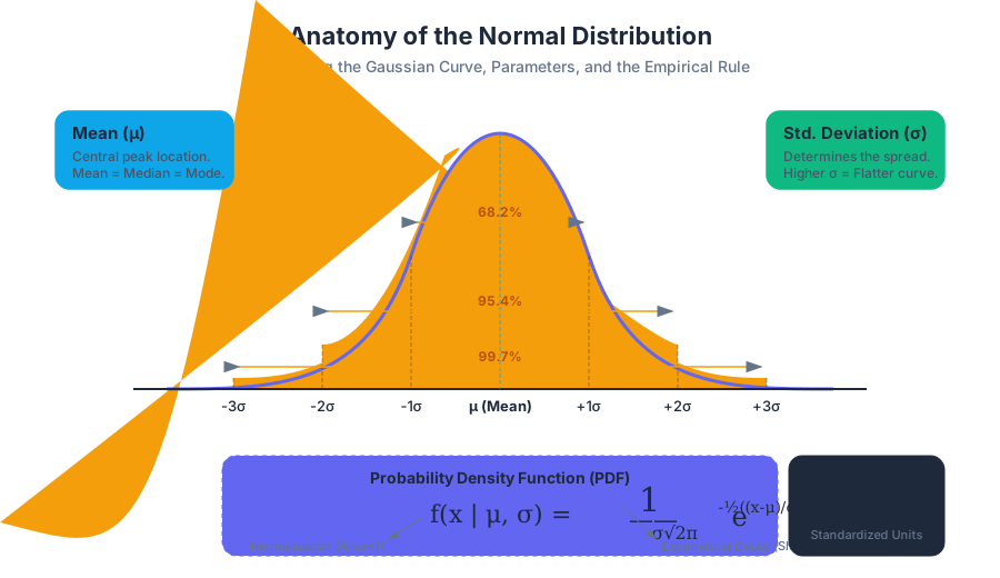
The Normal Distribution, often referred to as the Gaussian Distribution, is the most significant probability distribution in statistics. It describes a continuous probability distribution for a real-valued random variable characterized by its symmetrical, bell-shaped curve. From the heights of adult humans to the errors in scientific measurements and the fluctuations of stock market returns over short intervals, the normal distribution appears with such regularity that it is considered the "default" state of natural and social phenomena.

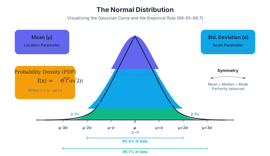
At its core, the normal distribution is defined by two parameters: the mean ($\mu$), which locates the peak of the distribution, and the standard deviation ($\sigma$), which measures the spread or "width" of the bell. Because the area under the curve represents the total probability of all possible outcomes, it must always equal 1.0 (or 100%).

1. Mathematical Foundation and the PDF

The shape of the normal distribution is governed by a specific mathematical function known as the Probability Density Function (PDF). Unlike discrete distributions where you can calculate the probability of a specific point, the PDF for a continuous distribution like the Normal Distribution gives the relative likelihood of a value. To find the actual probability, one must calculate the area under the curve between two points.

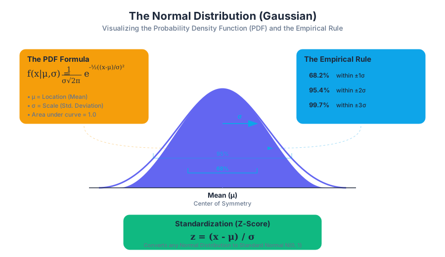
The Gaussian Function: For a random variable $X$, the probability density function is defined as: $$f(x | \mu, \sigma) = \frac{1}{\sigma\sqrt{2\pi}} e^{-\frac{1}{2}\left(\frac{x-\mu}{\sigma}\right)^2}$$

This formula reveals why the curve is symmetric: the term $(x-\mu)$ is squared, meaning that a value at a distance of $+d$ from the mean results in the same density as a value at $-d$.

Parameters of the Normal Distribution

Parameter	Symbol	Role	Impact on Graph
Mean	$\mu$	Location Parameter	Shifts the entire bell curve left or right along the x-axis.
Variance	$\sigma^2$	Scale Parameter	Determines the "flatness" or "sharpness" of the peak.
Standard Deviation	$\sigma$	Dispersion	The square root of variance; defines the units of distance from the mean.
Median/Mode	-	Central Tendency	In a perfect normal distribution, Mean = Median = Mode.

Implementation: Computing the PDF

In modern data science, we rarely calculate the PDF by hand. Instead, we use vectorized libraries to handle the exponential math.

import numpy as np

def calculate_normal_pdf(x, mu, sigma):
    """
    Computes the Probability Density Function (PDF) of a Normal Distribution.
    
    Args:
        x (float or np.array): The value(s) at which to evaluate the PDF.
        mu (float): The mean of the distribution.
        sigma (float): The standard deviation of the distribution.
    
    Returns:
        np.array: The probability density at each point in x.
    """
    # Pre-calculate the constant coefficient
    coefficient = 1 / (sigma * np.sqrt(2 * np.pi))
    
    # Calculate the exponent term
    exponent = np.exp(-0.5 * ((x - mu) / sigma) ** 2)
    
    return coefficient * exponent

# Example: Evaluating the density at the mean for a standard normal distribution
# mu=0, sigma=1, x=0 -> should be ~0.3989
print(f"Density at peak: {calculate_normal_pdf(0, 0, 1):.4f}")

2. The Standard Normal Distribution ($Z$)

While there are infinite possible normal distributions (any combination of $\mu$ and $\sigma$), the Standard Normal Distribution is a unique case where $\mu = 0$ and $\sigma = 1$. This specific distribution is denoted as $Z \sim N(0, 1)$.

The Standard Normal Distribution serves as a "universal translator" for statistics. By converting any normal distribution into the standard form, we can compare datasets that use different scales—such as comparing SAT scores (mean 1060) to ACT scores (mean 21).

The Z-Score Transformation

The process of converting a raw score ($x$) into a standard score is called Standardization. The resulting value is the Z-score.

Definition: A Z-score represents the number of standard deviations a data point is from the mean. A positive Z-score indicates the value is above the mean, while a negative Z-score indicates it is below.

\text{Z-score Formula: } z = \frac{x - \mu}{\sigma}

This transformation is linear. It shifts the distribution so the mean is at zero and scales it so the standard deviation is one. Crucially, standardization does not change the shape of the distribution; if the original data was skewed, the Z-scores will also be skewed.

3. The Empirical Rule (68-95-99.7 Rule)

One of the most powerful heuristics in statistics is the Empirical Rule. It provides a quick way to estimate probabilities without complex integration or Z-tables.

In any normal distribution:

1. 68.27% of the data falls within one standard deviation of the mean ($\mu \pm 1\sigma$).
2. 95.45% of the data falls within two standard deviations of the mean ($\mu \pm 2\sigma$).
3. 99.73% of the data falls within three standard deviations of the mean ($\mu \pm 3\sigma$).

Area Under the Curve Breakdown

Range	Z-score Range	Cumulative Probability	Percentage of Population
$\mu \pm 1\sigma$	$[-1, 1]$	$0.6827$	$\approx 68%$
$\mu \pm 2\sigma$	$[-2, 2]$	$0.9545$	$\approx 95%$
$\mu \pm 3\sigma$	$[-3, 3]$	$0.9973$	$\approx 99.7%$
$\mu \pm 6\sigma$	$[-6, 6]$	$0.999999998$	"Six Sigma" quality (near perfection)

4. Percentiles and Cumulative Probability

While Z-scores tell us "how far" a value is from the average, Percentiles tell us "how many" values are below it. The Cumulative Distribution Function (CDF) calculates the area under the normal curve from $-\infty$ to a specific point $x$.

For example, a Z-score of $0$ is the 50th percentile, because the distribution is symmetric and exactly half the data lies below the mean.

Common Critical Z-scores

In inferential statistics (like hypothesis testing), we often look for specific "tail" areas. These critical values are the foundation of confidence intervals.

Confidence Level	Alpha ($\alpha$)	Tail Area (One-sided)	Critical Z-score ($z^*$)
90%	0.10	0.05	1.645
95%	0.05	0.025	1.960
99%	0.01	0.005	2.576
99.9%	0.001	0.0005	3.291

Real-World Usage: SQL-based Z-score Analysis

In a production database, you might need to identify outliers in a transaction table by calculating Z-scores on the fly.

-- Identifying anomalous transaction amounts (Outliers > 3 sigma)
WITH Stats AS (
    SELECT 
        AVG(amount) AS mu, 
        STDDEV(amount) AS sigma 
    FROM transactions
    WHERE status = 'completed'
)
SELECT 
    t.transaction_id,
    t.amount,
    ((t.amount - s.mu) / s.sigma) AS z_score
FROM 
    transactions t, 
    Stats s
WHERE 
    ABS((t.amount - s.mu) / s.sigma) > 3.0;

5. Why the Normal Distribution is Everywhere: The Central Limit Theorem

The ubiquity of the normal distribution is not a coincidence; it is a mathematical necessity described by the Central Limit Theorem (CLT).

The Central Limit Theorem: Given a sufficiently large sample size from a population with a finite level of variance, the mean of all samples from the same population will be approximately equal to the mean of the population, and the distribution of those means will be approximately normal, regardless of the original population's distribution shape.

This is why the normal distribution is the "Gold Standard" for measurement. Even if individual events are binary (like a coin flip) or highly skewed (like household income), the average of many such events will inevitably settle into a bell curve.

6. Extensions: Comparing the Normal to Other Distributions

While the normal distribution is powerful, it is not always the correct model. Engineers and scientists must distinguish between "Normal-like" data and data that follows other patterns.

Distribution	Relationship to Normal	Use Case
Log-Normal	$ln(X)$ is normally distributed.	Income, file sizes, biological growth (values cannot be negative).
Student's T	Heavier tails than Normal.	Used when sample size is small ($n < 30$) and $\sigma$ is unknown.
Cauchy	"Pathological" distribution with no defined mean/variance.	Resonance behavior, rotating lines. Extreme outliers are common.
Binomial	Discrete.	Becomes Normal as $n$ increases (De Moivre–Laplace theorem).

7. Common Pitfalls and Misconceptions

Pitfall A: The "Fat Tail" Risk

In finance and risk management, assuming a normal distribution can be catastrophic. The normal distribution predicts that "Black Swan" events (6 or 7 standard deviations away) are effectively impossible (occurring once every few billion years). However, real-world market data often exhibits Leptokurtosis (fat tails), where extreme events happen much more frequently than the Gaussian model suggests.

Pitfall B: Testing for Normality

You cannot simply look at a histogram and assume it is normal. Professional analysis requires statistical tests:

1. Shapiro-Wilk Test: Best for smaller samples.
2. Kolmogorov-Smirnov Test: Compares your data to a theoretical normal CDF.
3. Q-Q Plot (Quantile-Quantile): A visual tool where normal data should fall along a straight 45-degree line.

Pitfall C: Standardizing Non-Normal Data

Applying a Z-score formula to data that is heavily skewed (like wealth distribution) will yield Z-scores, but those scores will not correspond to the percentiles of the Standard Normal Table. A Z-score of 2.0 only represents the 97.7th percentile if the underlying data is normal.

8. Worked Example: Manufacturing Quality Control

A factory produces steel rods. The target length is 100cm, with a standard deviation of 2cm. The distribution is normal. If a rod is rejected for being longer than 105cm, what percentage of rods are rejected?

1. Identify Parameters: $\mu = 100$, $\sigma = 2$, $x = 105$.
2. Calculate Z-score: $$z = \frac{105 - 100}{2} = \frac{5}{2} = 2.5$$
3. Lookup Probability: Using a Z-table or software, the area to the left of $z = 2.5$ is $0.9938$.
4. Find the Tail: Since we want the percentage longer than 105cm, we calculate $1 - 0.9938 = 0.0062$.
5. Conclusion: Approximately 0.62% of the rods will be rejected for being too long.

The Central Limit Theorem (CLT)

The Central Limit Theorem (CLT) is the foundational pillar of modern statistical inference. It provides the mathematical justification for why the Normal Distribution (the "Bell Curve") appears so frequently in the natural and social sciences. At its core, the CLT states that the sum (or mean) of a large number of independent, identically distributed (i.i.d.) random variables will tend toward a normal distribution, regardless of the shape of the underlying population distribution.

This theorem transforms statistics from a purely descriptive exercise into a predictive science. Without the CLT, we would be unable to calculate confidence intervals or perform hypothesis tests for complex systems where the underlying probability density function (PDF) is unknown or non-normal.

The Foundation: The Law of Large Numbers (LLN)

Before diving into the CLT, one must understand the Law of Large Numbers (LLN). While the CLT describes the shape of the distribution of sample means, the LLN describes where that distribution is centered.

The Law of Large Numbers: As the number of trials or observations ($n$) increases, the sample mean ($\bar{X}$) converges to the theoretical population mean ($\mu$).

There are two distinct flavors of this law that mathematicians distinguish based on the "strength" of the convergence:

1. Weak Law of Large Numbers (WLLN): States that for any non-zero margin, the probability that the sample mean differs from the population mean approaches zero as $n \to \infty$. This is convergence in probability.
2. Strong Law of Large Numbers (SLLN): States that the sample mean converges to the population mean "almost surely." This means the probability that the sequence of means converges to $\mu$ is equal to 1.

LLN vs. CLT: A Critical Distinction

Feature	Law of Large Numbers (LLN)	Central Limit Theorem (CLT)
Primary Focus	Convergence of the mean value.	Convergence of the distribution shape.
Result	$\bar{X} \to \mu$	$\bar{X} \approx \mathcal{N}(\mu, \sigma^2/n)$
Utility	Guarantees stability of long-term averages.	Enables probabilistic inference and error estimation.
Requirement	Finite first moment (Mean exists).	Finite second moment (Variance exists).

The Mechanics of the Sampling Distribution

To understand the CLT, we must first define the Sampling Distribution. This is not the distribution of the raw data itself, but a "meta-distribution" of a statistic (like the mean) calculated from repeated samples of size $n$.

Imagine a population of 1 million people. If we take a sample of 100 people and calculate their average height, that single average is one data point in our sampling distribution. If we repeat this process 10,000 times, the resulting histogram of those 10,000 averages will form the sampling distribution.

Properties of the Sampling Distribution of the Mean

As $n$ increases, the sampling distribution exhibits three predictable behaviors:

1. Center: The mean of the sampling distribution ($\mu_{\bar{x}}$) is equal to the mean of the population ($\mu$).
2. Spread: The standard deviation of the sampling distribution, known as the Standard Error (SE), decreases as the sample size increases.
3. Shape: The distribution becomes increasingly Gaussian (Normal), even if the population is heavily skewed or discrete.

The Standard Error: Quantifying Precision

The Standard Error (SE) is the standard deviation of the sampling distribution. It measures how much the sample mean is expected to vary from the true population mean.

Definition: The Standard Error of the Mean (SEM) is calculated as: $$SE = \frac{\sigma}{\sqrt{n}}$$ Where $\sigma$ is the population standard deviation and $n$ is the sample size.

This formula reveals the Square Root Law: to cut your measurement error in half, you must quadruple your sample size. This is a fundamental constraint in experimental design and polling.

Comparison of Standard Deviation and Standard Error

Metric	Symbol	Description	Relationship to $n$
Standard Deviation	$\sigma$	Measures the dispersion of individual data points in the population.	Independent of $n$.
Sample Std Dev	$s$	An estimate of $\sigma$ derived from a single sample.	Becomes a better estimate as $n$ grows.
Standard Error	$SE$	Measures the dispersion of sample means around the true mean.	Inversely proportional to $\sqrt{n}$.

Formal Statement of the Central Limit Theorem

In its most common form (the Lindeberg-Lévy CLT), the theorem is stated as follows:

Suppose ${X_1, X_2, \dots, X_n}$ is a sequence of i.i.d. random variables with $E[X_i] = \mu$ and $Var[X_i] = \sigma^2 < \infty$. As $n$ approaches infinity, the random variables $\sqrt{n}(\bar{X}_n - \mu)$ converge in distribution to a normal distribution $\mathcal{N}(0, \sigma^2)$:

$$\bar{X}_n \xrightarrow{d} \mathcal{N}\left(\mu, \frac{\sigma^2}{n}\right)$$

Implementation: Simulating the CLT in Python

The following implementation demonstrates the CLT by sampling from a highly non-normal distribution (an Exponential distribution) and showing how the distribution of the means converges to a Normal curve.

import numpy as np
import matplotlib.pyplot as plt

def simulate_clt(population_dist, sample_sizes, iterations=10000):
    """
    Simulates the Central Limit Theorem by taking repeated samples
    of varying sizes from a non-normal population.
    """
    fig, axes = plt.subplots(1, len(sample_sizes), figsize=(15, 5))
    
    # Generate a non-normal population (Exponential)
    if population_dist == 'exp':
        population = np.random.exponential(scale=1.0, size=100000)
        mu, sigma = 1.0, 1.0
    
    for i, n in enumerate(sample_sizes):
        # Calculate 'iterations' number of sample means
        means = [np.mean(np.random.choice(population, size=n)) for _ in range(iterations)]
        
        # Plotting the sampling distribution
        axes[i].hist(means, bins=50, density=True, color='skyblue', edgecolor='black', alpha=0.7)
        axes[i].set_title(f'Sample Size n={n}')
        
        # Overlay the theoretical Normal curve
        x = np.linspace(min(means), max(means), 100)
        theoretical_se = sigma / np.sqrt(n)
        y = (1 / (theoretical_se * np.sqrt(2 * np.pi))) * \
            np.exp(-0.5 * ((x - mu) / theoretical_se)**2)
        axes[i].plot(x, y, color='red', lw=2)

    plt.tight_layout()
    plt.show()

# Execute simulation for n = 2, 10, 50
simulate_clt('exp', [2, 10, 50])

Mathematical Derivation via Characteristic Functions

To truly understand why the CLT works, we look at Characteristic Functions ($\phi_X(t)$). The characteristic function of a random variable is the Fourier transform of its probability density function. A key property is that the characteristic function of the sum of independent variables is the product of their individual characteristic functions.

The Proof Sketch

1. Let $Z_n = \frac{\sum X_i - n\mu}{\sigma\sqrt{n}}$ be the normalized sum.
2. The characteristic function of a single normalized variable $Y_i = \frac{X_i - \mu}{\sigma}$ can be expanded using a Taylor series around 0: $$\phi_Y(t) = 1 - \frac{t^2}{2} + o(t^2)$$
3. The characteristic function of the sum $Z_n$ is: $$\phi_{Z_n}(t) = \left[ \phi_Y\left(\frac{t}{\sqrt{n}}\right) \right]^n = \left[ 1 - \frac{t^2}{2n} + o\left(\frac{t^2}{n}\right) \right]^n$$
4. As $n \to \infty$, this expression takes the form of the definition of the exponential function $(1 + \frac{x}{n})^n \to e^x$: $$\lim_{n \to \infty} \phi_{Z_n}(t) = e^{-t^2/2}$$
5. The result $e^{-t^2/2}$ is exactly the characteristic function of the Standard Normal Distribution $\mathcal{N}(0, 1)$.

\begin{aligned}
\text{Let } X_i \text{ be i.i.d. with } E[X] = 0, Var[X] = 1 \\
\text{Characteristic Function: } \varphi_X(t) = E[e^{itX}] \\
\varphi_{\sum X_i / \sqrt{n}}(t) = \left[ \varphi_X\left(\frac{t}{\sqrt{n}}\right) \right]^n \\
\text{Taylor Expansion: } \varphi_X(s) = 1 - \frac{s^2}{2} + R(s) \\
\left[ 1 - \frac{t^2}{2n} + R\left(\frac{t}{\sqrt{n}}\right) \right]^n \xrightarrow{n \to \infty} e^{-t^2/2}
\end{aligned}

Practical Application: Confidence Intervals in Engineering

In structural engineering, the strength of a batch of steel bolts might not be normally distributed. However, when calculating the average strength of the 50 bolts used in a critical joint, the CLT allows engineers to use the Normal distribution to calculate the probability of failure.

Example Calculation

Suppose a manufacturer claims bolts have a mean breaking strength of 10,000 psi with a standard deviation of 400 psi. You test a sample of 64 bolts. What is the probability the sample mean is less than 9,900 psi?

1. Identify Parameters: $\mu = 10,000$, $\sigma = 400$, $n = 64$.
2. Calculate Standard Error: $SE = \frac{400}{\sqrt{64}} = \frac{400}{8} = 50$.
3. Calculate Z-score: $Z = \frac{\bar{X} - \mu}{SE} = \frac{9,900 - 10,000}{50} = -2.0$.
4. Find Probability: Using a standard normal table, $P(Z < -2.0) \approx 0.0228$.

There is a 2.28% chance that the sample mean would be this low if the manufacturer's claim is true.

# Using 'R' from the command line to calculate the p-value for the example above
Rscript -e "pnorm(9900, mean=10000, sd=400/sqrt(64))"

# Output:
# [1] 0.02275013

Variations and Extensions

While the Lindeberg-Lévy CLT is the most famous, several variations exist for different conditions:

Variation	Condition	Key Insight
Lyapunov CLT	Non-identical distributions.	Variables don't need the same distribution, provided no single variable dominates the variance.
Martingale CLT	Dependent variables.	CLT holds for sequences where the next value depends on the current state, given certain constraints.
Multivariate CLT	Vector-valued variables.	The vector of means converges to a Multivariate Normal distribution with a specific Covariance Matrix.
Berry-Esseen Theorem	Finite third moment.	Provides a bound on the speed of convergence, telling us how large $n$ must be for a given accuracy.

Common Pitfalls and Misconceptions

Despite its power, the CLT is frequently misunderstood. Senior practitioners must be aware of these edge cases:

1. The "n = 30" Myth

Introductory textbooks often state that $n \ge 30$ is sufficient for the CLT to apply. This is a heuristic, not a rule.

• If the population is Symmetric and Unimodal, $n=5$ might be enough.
• If the population is Highly Skewed (e.g., wealth distribution), $n=500$ might be insufficient.
• If the population has Fat Tails (e.g., Cauchy distribution), the CLT never applies because the variance is infinite.

2. Confusing the Population with the Sample Mean

A common mistake is thinking that as $n$ increases, the population distribution becomes normal. This is false. The population distribution is fixed. Only the sampling distribution of the mean becomes normal.

3. Independence Assumption

The CLT requires observations to be independent. In time-series data or clustered samples (e.g., students within the same classroom), observations are often correlated. In these cases, the standard error will be underestimated, leading to overconfidence in the results (spurious significance).

4. The "Average" Trap

The CLT applies to sums and means. It does not apply to other statistics like the maximum, minimum, or range. For example, the distribution of the maximum value in a sample follows the Generalized Extreme Value (GEV) distribution, not the Normal distribution.

Summary of Convergence

Concept	Type of Convergence	What is Converging?
LLN	Convergence in Probability / Almost Surely	The value of $\bar{X}$ to a constant $\mu$.
CLT	Convergence in Distribution	The functional form of the PDF to a Gaussian.
Slutsky's Theorem	Algebraic Convergence	Combinations of sequences (e.g., $X_n + Y_n$) converge predictably.

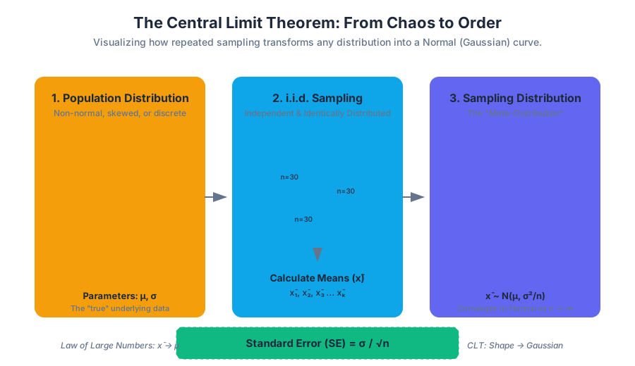
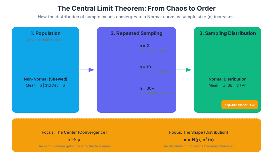
Confidence Intervals

In frequentist statistics, we are often tasked with estimating an unknown population parameter (such as a mean $\mu$ or a proportion $p$) based on a finite sample. While a Point Estimate provides a single "best guess," it offers no information regarding the precision or reliability of that guess. A Confidence Interval (CI) addresses this by providing a range of plausible values for the parameter, accompanied by a quantitative measure of certainty.

The Philosophy of Interval Estimation

The transition from point estimation to interval estimation represents a shift from "finding a value" to "quantifying uncertainty." If we report that the average height of a population is 175 cm, we provide no context on whether that estimate is based on five people or five thousand. A confidence interval contextualizes the estimate by incorporating the variability of the data and the size of the sample.

Definition: A Confidence Interval is an interval of the form $(\text{point estimate} - \text{margin of error}, \text{point estimate} + \text{margin of error})$. It is designed to contain the true population parameter with a specified probability, known as the Confidence Level.

The Frequentist Interpretation

A common misconception is that a 95% confidence interval has a 95% probability of containing the true parameter. Technically, in frequentist statistics, the population parameter is a fixed (though unknown) constant. It is the interval that is the random variable.

• Correct Interpretation: If we were to repeat the sampling process 100 times and calculate a 95% confidence interval for each sample, approximately 95 of those intervals would contain the true population parameter.

Key Components of a Confidence Interval

To construct an interval, four primary components must be synthesized: the point estimate, the confidence level, the standard error, and the critical value.

Component	Symbol	Description
Point Estimate	$\bar{x}$ or $\hat{p}$	The sample statistic used as the center of the interval.
Confidence Level	$1 - \alpha$	The success rate of the method (usually 0.90, 0.95, or 0.99).
Alpha (Significance)	$\alpha$	The probability that the interval does not contain the parameter.
Standard Error	$SE$	The standard deviation of the sampling distribution of the statistic.
Critical Value	$z^$ or $t^$	The number of standard errors move away from the mean to capture the desired area.
Margin of Error	$EBM$ or $E$	The product of the critical value and the standard error ($z^* \times SE$).

1. The Point Estimate

The Point Estimate is the specific value calculated from the sample. For a population mean $\mu$, the point estimate is the sample mean $\bar{x}$. For a population proportion $P$, it is the sample proportion $\hat{p} = x/n$.

2. The Confidence Level ($1 - \alpha$)

The Confidence Level represents the long-term success rate of the estimation procedure. If $1 - \alpha = 0.95$, then $\alpha = 0.05$. This $\alpha$ is the "area in the tails" of the probability distribution that we are willing to exclude.

3. The Margin of Error (EBM)

Also known as the Error Bound for a Population Mean (EBM), this is the distance from the point estimate to the interval boundaries. It is the "plus-minus" part of the statistic.

The Mathematics of the Interval

The construction of a confidence interval relies on the Central Limit Theorem (CLT), which states that for a sufficiently large sample size, the sampling distribution of the mean will be approximately normal, regardless of the population's distribution.

Case A: Known Population Standard Deviation ($\sigma$)

When the population standard deviation $\sigma$ is known, we use the Z-distribution (Standard Normal).

CI = \bar{x} \pm z_{\alpha/2} \left( \frac{\sigma}{\sqrt{n}} \right)

Case B: Unknown Population Standard Deviation ($s$)

In practice, $\sigma$ is rarely known. We must estimate it using the sample standard deviation $s$. This introduces extra uncertainty, especially in small samples. To account for this, we use the Student's T-Distribution.

CI = \bar{x} \pm t_{\alpha/2, df} \left( \frac{s}{\sqrt{n}} \right)

Where $df = n - 1$ (degrees of freedom).

The Student's T-Distribution

Developed by William Sealy Gosset (under the pseudonym "Student") while working for the Guinness Brewery, the T-distribution is essential when sample sizes are small ($n < 30$) or the population variance is unknown.

Characteristics of the T-Distribution

1. Bell-shaped and Symmetric: Like the Z-distribution, it is centered at zero.
2. Heavier Tails: The T-distribution has more probability in its tails than the Z-distribution. This reflects the added uncertainty of estimating $\sigma$ with $s$.
3. Degrees of Freedom ($df$): As $n$ increases, the T-distribution approaches the Standard Normal distribution. With infinite degrees of freedom, $t = z$.

Sample Size ($n$)	$df$	Critical Value ($t^*$) for 95% CI	Critical Value ($z^*$) for 95% CI
5	4	2.776	1.960
10	9	2.262	1.960
30	29	2.045	1.960
100	99	1.984	1.960
$\infty$	$\infty$	1.960	1.960

Implementation: Calculating a Confidence Interval

To calculate a confidence interval for a mean where the population standard deviation is unknown, we follow a systematic algorithmic approach.

Low-Level Python Implementation (NumPy/SciPy)

This example demonstrates the manual calculation of the interval components to illustrate the underlying mechanics.

import numpy as np
from scipy import stats

def calculate_confidence_interval(data, confidence=0.95):
    """
    Calculates the confidence interval for a sample mean using 
    the T-distribution (unknown sigma).
    """
    n = len(data)
    mean = np.mean(data)
    sem = stats.sem(data)  # Standard Error of the Mean: s / sqrt(n)
    
    # Calculate degrees of freedom
    df = n - 1
    
    # Find the critical t-value
    # ppf: Percent Point Function (inverse of CDF)
    # We use (1 + confidence) / 2 to find the upper tail cutoff
    t_crit = stats.t.ppf((1 + confidence) / 2, df)
    
    # Calculate Margin of Error
    margin_of_error = t_crit * sem
    
    lower_bound = mean - margin_of_error
    upper_bound = mean + margin_of_error
    
    return {
        "point_estimate": mean,
        "margin_of_error": margin_of_error,
        "interval": (lower_bound, upper_bound),
        "t_critical": t_crit,
        "df": df
    }

# Example: Weights of 15 randomly selected components (in grams)
sample_data = [10.2, 9.8, 10.5, 10.1, 9.9, 10.3, 10.0, 9.7, 10.4, 10.2, 10.1, 9.8, 10.2, 10.0, 10.1]
result = calculate_confidence_interval(sample_data)

print(f"Estimate: {result['point_estimate']:.3f} ± {result['margin_of_error']:.3f}")
print(f"95% CI: {result['interval']}")

Confidence Intervals for Proportions

When dealing with categorical data (e.g., "Yes/No" surveys), we estimate the population proportion $P$. The point estimate is $\hat{p} = x/n$.

Requirements for Normality

To use the Normal approximation for proportions, the Success-Failure Condition must be met:

• $np \geq 10$
• $n(1-p) \geq 10$

Derivation of the Proportion Interval

The standard error for a proportion is $\sqrt{\frac{\hat{p}(1-\hat{p})}{n}}$.

\text{Step 1: Identify } \hat{p} = \frac{x}{n}
\text{Step 2: Identify } \hat{q} = 1 - \hat{p}
\text{Step 3: Calculate } SE = \sqrt{\frac{\hat{p}\hat{q}}{n}}
\text{Step 4: Find } z_{\alpha/2} \text{ for the confidence level.}
\text{Step 5: } CI = \hat{p} \pm z_{\alpha/2} \cdot SE

High-Level Usage (R Language)

In statistical computing environments like R, these intervals are often calculated using built-in high-level functions that handle edge cases (like the continuity correction).

# Scenario: 400 people are surveyed, 220 support a new policy.
# Calculate a 95% confidence interval for the population proportion.

successes <- 220
total_n <- 400

# Using prop.test (Wilson score interval by default, which is more robust)
result <- prop.test(x = successes, n = total_n, conf.level = 0.95)

print(result$conf.int)
# Output: [1] 0.5001243 0.5985012
# Interpretation: We are 95% confident the true support is between 50% and 59.8%.

Factors Affecting Interval Width

The width of a confidence interval is a proxy for the precision of our estimate. A narrower interval indicates higher precision.

Factor	Change	Effect on Interval Width	Reason
Confidence Level	Increase (90% $\to$ 99%)	Wider	To be more certain, we must include more possible values.
Sample Size ($n$)	Increase	Narrower	Larger samples reduce the standard error ($\sqrt{n}$ is in the denominator).
Variability ($s$ or $\sigma$)	Increase	Wider	More "noise" in the data makes the estimate less certain.

Determining Required Sample Size

One of the most practical applications of CI theory is determining how many subjects are needed for a study before data collection begins. This is done by specifying a desired Margin of Error ($E$).

For Means:

To solve for $n$, we rearrange the EBM formula: $E = z \frac{\sigma}{\sqrt{n}} \implies \sqrt{n} = \frac{z \sigma}{E} \implies n = \left( \frac{z \sigma}{E} \right)^2$

For Proportions:

$n = \frac{z^2 \hat{p} \hat{q}}{E^2}$ Note: If no preliminary $\hat{p}$ is known, use $0.5$ as a conservative estimate, as it maximizes the required $n$.

CLI Example: Quick Sample Size Calculation

Using a simple shell command with bc (arbitrary precision calculator) to find $n$ for a proportion with $E=0.03$ at 95% confidence ($z=1.96$):

# Formula: (z^2 * p * q) / E^2
# p=0.5, q=0.5, z=1.96, E=0.03
echo "scale=2; (1.96^2 * 0.5 * 0.5) / (0.03^2)" | bc
# Output: 1067.11
# Rule: Always round UP for sample size. Result = 1068.

Common Pitfalls and Misconceptions

1. The "Probability" Trap

As noted earlier, once an interval is calculated (e.g., [10, 20]), the probability that the parameter is in that specific interval is either 0 or 1. The "95%" refers to the reliability of the process, not the specific result.

2. Over-reliance on $n=30$

While 30 is a common rule of thumb for the Central Limit Theorem, it is not a magic number. If the underlying population is extremely skewed or contains heavy outliers, much larger samples may be required for the Z or T distributions to be valid.

3. Standard Deviation vs. Standard Error

• Standard Deviation ($s$): Measures the dispersion of individual data points.
• Standard Error ($SE$): Measures the dispersion of the sample mean from the population mean. Confidence intervals always use the Standard Error.

4. Confusing CI with Prediction Intervals

A Confidence Interval estimates where the mean of the population lies. A Prediction Interval estimates where a single future observation will lie. Prediction intervals are significantly wider because they must account for both the uncertainty in the mean and the inherent variability of individuals.

Advanced Variations

Bootstrap Confidence Intervals

When the underlying distribution is unknown and the sample size is small, we can use Bootstrapping. This involves resampling the data with replacement thousands of times to generate an empirical sampling distribution. The 2.5th and 97.5th percentiles of this distribution form the 95% CI.

Bayesian Credible Intervals

Unlike Frequentist CIs, Bayesian Credible Intervals do allow for probability statements about the parameter. By combining a "Prior" belief with the "Likelihood" of the data, Bayesians produce a "Posterior" distribution. A 95% Credible Interval is the range that contains 95% of the posterior probability.

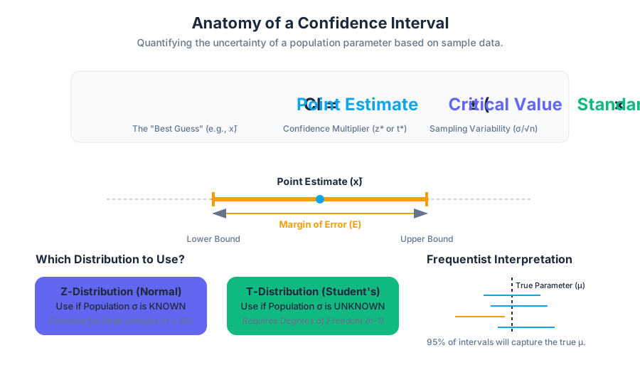
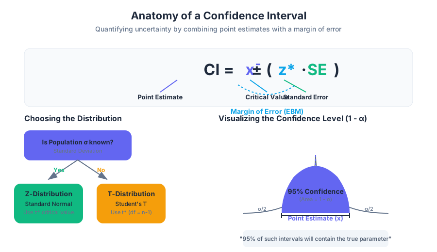
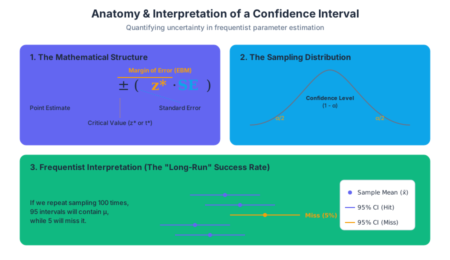
Hypothesis Testing with One Sample

Hypothesis testing is the formal statistical backbone of the scientific method. It provides a rigorous framework for moving beyond mere observation into the realm of inferential statistics, where we use sample data to make probabilistic statements about an entire population. At its core, hypothesis testing is a "proof by contradiction" mechanism: we assume a default state of the world (the Null Hypothesis) and determine if our observed data is so unlikely under that assumption that we are forced to reject it in favor of a new explanation.

In a one-sample context, we are typically comparing a single sample mean ($\bar{x}$) or proportion ($\hat{p}$) against a known or hypothesized population parameter ($\mu_0$ or $p_0$). This process is essential in quality control, medical research, and A/B testing, where one must decide if a deviation from the norm is a genuine effect or simply the result of stochastic noise.

The Logical Framework: $H_0$ and $H_a$

The foundation of any test lies in the construction of two mutually exclusive and collectively exhaustive statements.

The Null Hypothesis ($H_0$)

The Null Hypothesis represents the status quo, the "no-effect" state, or the assumption that any observed difference is due to chance. In a one-sample test, $H_0$ always contains an equality ($=, \le, \text{ or } \ge$).

The Alternative Hypothesis ($H_a$)

The Alternative Hypothesis (sometimes denoted as $H_1$) is the claim the researcher hopes to support. It represents a departure from the status quo. $H_a$ never contains an equality ($<, >, \text{ or } \neq$).

Hypothesis Type	Notation	Logical Role	Mathematical Symbols
Null	$H_0$	The "Innocent" plea; the baseline assumption.	$=, \leq, \geq$
Alternative	$H_a$	The "Guilty" verdict; the research claim.	$\neq, >, <$

The Burden of Proof: In the Frequentist tradition, the burden of proof lies entirely on the Alternative Hypothesis. We do not "accept" the Null; we merely "fail to reject" it if the evidence is insufficient. This is analogous to a court of law where a defendant is found "not guilty" rather than "innocent."

The Decision Calculus: P-values and Alpha ($\alpha$)

To decide between $H_0$ and $H_a$, we need a threshold for "unlikeliness."

Significance Level ($\alpha$)

The Significance Level ($\alpha$) is the probability threshold set by the researcher before the experiment. It defines the maximum risk of rejecting a true null hypothesis that the researcher is willing to take. Common values include 0.05, 0.01, and 0.10.

The P-value

The P-value is the probability of obtaining a test statistic at least as extreme as the one observed, assuming the null hypothesis is true. It is NOT the probability that the null hypothesis is true; rather, it is $P(\text{Data} | H_0)$.

Decision Rules

• If P-value $\le \alpha$: The result is statistically significant. Reject $H_0$.
• If P-value $> \alpha$: The result is not statistically significant. Fail to reject $H_0$.

Statistical Error Theory: Type I and Type II

Because we are working with samples rather than entire populations, our decisions are subject to two types of errors.

1. Type I Error ($\alpha$): Rejecting $H_0$ when it is actually true (a "False Positive").
2. Type II Error ($\beta$): Failing to reject $H_0$ when it is actually false (a "False Negative").

Reality \ Decision	Fail to Reject $H_0$	Reject $H_0$
$H_0$ is True	Correct Decision (Confidence: $1-\alpha$)	Type I Error (Significance: $\alpha$)
$H_0$ is False	Type II Error ($\beta$)	Correct Decision (Power: $1-\beta$)

The Power of a Test

The Power of a statistical test ($1 - \beta$) is the probability that the test will correctly reject a false null hypothesis. Increasing the sample size ($n$) or the effect size generally increases the power of the test.

Mechanics of the One-Sample Test

The choice of test depends on whether the population standard deviation ($\sigma$) is known and whether the sample size is large enough for the Central Limit Theorem to apply.

1. The One-Sample Z-Test

Used when the population variance $\sigma^2$ is known and the population is normally distributed or the sample size $n$ is large ($n \ge 30$).

2. The One-Sample T-Test

Used when the population variance $\sigma^2$ is unknown (which is almost always the case in practice). It uses the sample standard deviation ($s$) and follows the Student's t-distribution with $n-1$ degrees of freedom ($df$).

Code Example 1: Low-Level Implementation (Python)

This snippet demonstrates the manual calculation of a T-statistic and P-value from raw data, illustrating the underlying mechanics.

import math
from scipy import stats

def perform_one_sample_t_test(data, hypothesized_mean):
    """
    Manually calculates a one-sample T-test.
    """
    n = len(data)
    sample_mean = sum(data) / n
    
    # Calculate sample variance and standard deviation
    variance = sum((x - sample_mean) ** 2 for x in data) / (n - 1)
    sample_std = math.sqrt(variance)
    
    # Standard Error of the Mean (SEM)
    sem = sample_std / math.sqrt(n)
    
    # T-statistic calculation: (Observed - Hypothesized) / SE
    t_stat = (sample_mean - hypothesized_mean) / sem
    
    # Degrees of freedom
    df = n - 1
    
    # P-value calculation (two-tailed)
    # stats.t.cdf gives the area to the left
    p_value = 2 * (1 - stats.t.cdf(abs(t_stat), df))
    
    return {
        "mean": sample_mean,
        "t_statistic": t_stat,
        "p_value": p_value,
        "df": df
    }

# Real-world scenario: Testing if a machine fills 500ml bottles correctly
bottle_volumes = [498, 502, 505, 497, 503, 500, 499, 501, 504, 496]
results = perform_one_sample_t_test(bottle_volumes, 500)

print(f"T-Stat: {results['t_statistic']:.4f}, P-Val: {results['p_value']:.4f}")

Code Example 2: Mathematical Derivation (LaTeX/Math)

The following represents the formal derivation of the test statistic and the probability density function for the T-distribution.

\text{The Test Statistic for a One-Sample T-Test is defined as:}
\\
t = \frac{\bar{x} - \mu_0}{s / \sqrt{n}}
\\
\text{Where:}
\begin{cases} 
\bar{x} & \text{Sample Mean} \\
\mu_0 & \text{Hypothesized Population Mean} \\
s & \text{Sample Standard Deviation} \\
n & \text{Sample Size} 
\end{cases}
\\
\text{The Probability Density Function (PDF) of the T-distribution with } \nu \text{ degrees of freedom:}
\\
f(t) = \frac{\Gamma(\frac{\nu+1}{2})}{\sqrt{\nu\pi}\,\Gamma(\frac{\nu}{2})} \left(1+\frac{t^2}{\nu}\right)^{-\frac{\nu+1}{2}}

Step-by-Step Execution of a One-Sample Test

To ensure scientific validity, a hypothesis test must follow a standardized pipeline.

Step 1: State the Hypotheses

Define $H_0$ and $H_a$ clearly. Determine if the test is one-tailed (directional, e.g., "greater than") or two-tailed (non-directional, e.g., "different from").

Step 2: Set the Criteria

Choose the significance level $\alpha$. In high-stakes fields like pharmaceuticals, $\alpha$ might be 0.01; in social sciences, 0.05 is standard.

Step 3: Verify Assumptions

• Independence: Observations must be independent of each other.
• Randomness: Data should be collected via a random sampling method.
• Normality: The population should be normally distributed, or $n$ should be large enough (Central Limit Theorem).

Step 4: Calculate the Test Statistic and P-value

Compute the Z or T score and find the corresponding P-value using distribution tables or software.

Step 5: Make the Decision

Compare the P-value to $\alpha$ and state the conclusion in the context of the original problem.

Component	Two-Tailed Test	One-Tailed Test (Right)	One-Tailed Test (Left)
$H_a$	$\mu \neq \mu_0$	$\mu > \mu_0$	$\mu < \mu_0$
Rejection Region	Both tails	Right tail	Left tail
P-value Calc	$2 \times P(T >	t	)$

Code Example 3: High-Level Implementation (R)

R is the lingua franca of statistics. A one-sample T-test that takes lines of code in other languages is a single function call here.

# Scenario: Testing if the average weight of a new breed of apple is 150g
apple_weights <- c(145, 152, 158, 148, 153, 155, 149, 151, 160, 147)

# Perform a one-sample T-test
# mu = hypothesized mean
# conf.level = 1 - alpha
test_result <- t.test(apple_weights, mu = 150, conf.level = 0.95)

# Output the results
print(test_result)

# Accessing specific components
cat("P-value is:", test_result$p.value, "\n")
cat("95% Confidence Interval:", test_result$conf.int[1], "to", test_result$conf.int[2], "\n")

Critical Extensions: Effect Size and Confidence Intervals

A common pitfall in hypothesis testing is over-reliance on the P-value. With a large enough sample size, even a trivial difference can become "statistically significant." To counter this, we use Effect Size.

Cohen's $d$

Cohen's $d$ measures the magnitude of the difference in terms of standard deviations. $$d = \frac{|\bar{x} - \mu_0|}{s}$$

Effect Size	Cohen's $d$ Value
Small	0.2
Medium	0.5
Large	0.8

Confidence Intervals (CI)

A Confidence Interval provides a range of plausible values for the population parameter. If the hypothesized mean $\mu_0$ falls outside the $(1-\alpha)$ confidence interval, we reject $H_0$ at the $\alpha$ level.

Common Pitfalls and Misconceptions

1. "P-hacking": Running multiple tests or adjusting the sample size until a significant P-value is found. This inflates the Type I error rate.
2. Misinterpreting the P-value: Thinking a P-value of 0.05 means there is a 95% chance the alternative hypothesis is true.
3. Absence of Evidence vs. Evidence of Absence: Failing to reject $H_0$ does not prove $H_0$ is true; it simply means the data is not strong enough to prove otherwise.
4. Statistical vs. Practical Significance: A result can be statistically significant ($p < 0.05$) but practically useless if the effect size is near zero.

Code Example 4: Data Pre-processing (SQL)

Before running a hypothesis test, data engineers often use SQL to validate assumptions like sample size and basic distribution stats.

-- Checking if we have enough data points and basic stats for a specific group
-- to ensure the Central Limit Theorem (n >= 30) is satisfied.
SELECT 
    product_line,
    COUNT(weight) AS sample_size,
    AVG(weight) AS sample_mean,
    STDDEV(weight) AS sample_stddev,
    -- Calculate the Standard Error of the Mean
    STDDEV(weight) / SQRT(COUNT(weight)) AS standard_error
FROM 
    factory_production_logs
WHERE 
    timestamp >= '2023-01-01'
GROUP BY 
    product_line
HAVING 
    COUNT(weight) >= 30;

Summary of the Decision Matrix

When approaching a one-sample problem, use this logic flow:

1. Is the data continuous? (If yes, proceed to Means. If no, use Proportions).
2. Is $\sigma$ known? (If yes, use Z-test. If no, use T-test).
3. Is $n < 30$? (If yes, the population must be normal to use the T-test).
4. Is the claim directional? (If yes, use a one-tailed test).

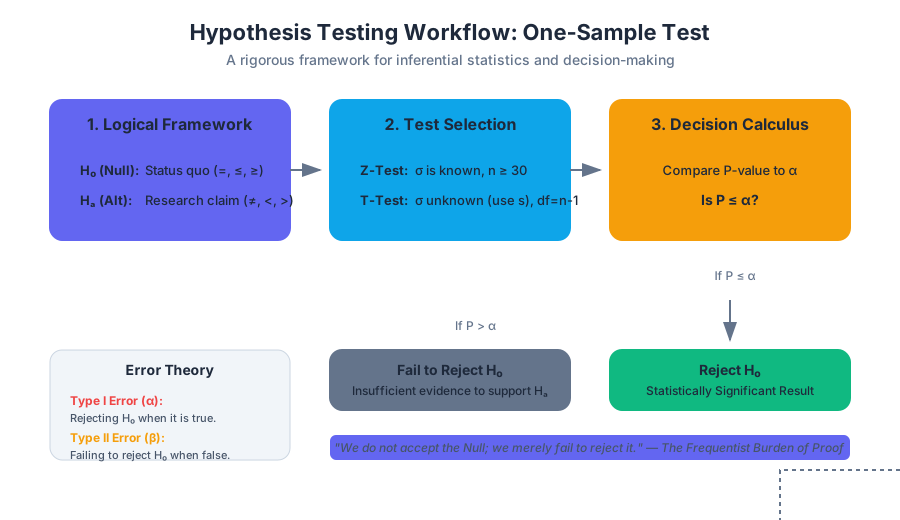
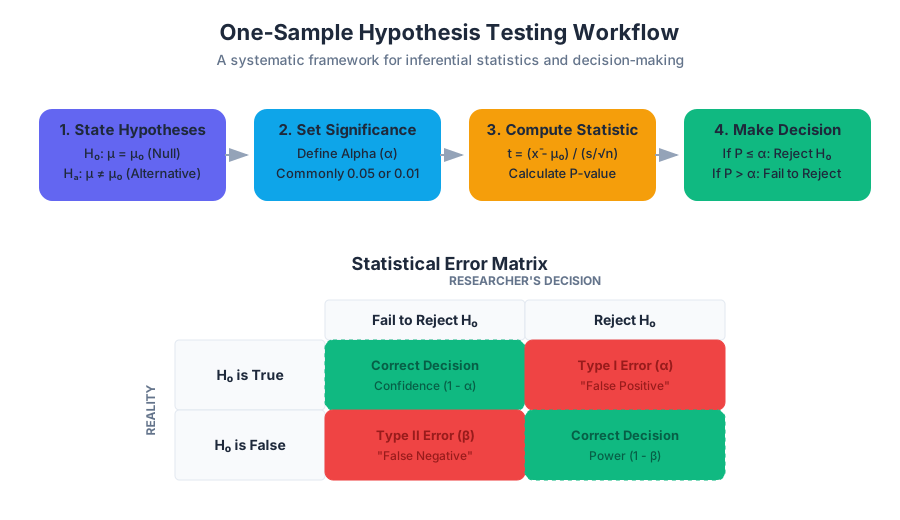
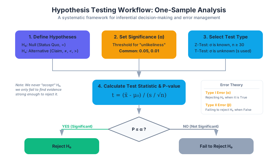
Hypothesis Testing with Two Samples

In the landscape of statistical inference, single-sample testing serves as a foundational proof of concept. However, empirical science rarely operates in a vacuum. The most critical questions in medicine, engineering, and social science are comparative: Does Drug A outperform Drug B? Does a new manufacturing process reduce defects compared to the legacy system? Do two demographic groups exhibit different behavioral patterns?

Hypothesis testing with two samples allows us to determine if the observed differences between two groups are statistically significant or merely the result of stochastic noise. This requires a sophisticated understanding of how variances interact, how samples are related, and how the geometry of the sampling distribution changes when we move from a single point estimate to a difference of estimates.

The Taxonomy of Two-Sample Tests

Before selecting a mathematical model, a researcher must identify the relationship between the two samples and the nature of the data. The choice of test is governed by three primary factors: the independence of the groups, the equality of their variances, and the type of data (means vs. proportions).

Test Type	Data Requirement	Relationship	Key Statistic
Independent t-test (Welch’s)	Continuous	Unrelated groups	Difference of means, unequal variance
Pooled Variance t-test	Continuous	Unrelated groups	Difference of means, equal variance
Paired/Matched t-test	Continuous	Related/Same subjects	Mean of differences
Two-Proportion z-test	Categorical/Binary	Unrelated groups	Difference of proportions

---

Independent Samples: Comparing Unrelated Means

Independent samples occur when the subjects in one group provide no information about the subjects in the second group. For example, testing the blood pressure of a group in New York versus a group in Tokyo.

The Aspin-Welch T-Test (Unequal Variance)

In modern computational statistics, the Aspin-Welch t-test is the default choice. Unlike the classical Student’s t-test, it does not assume that the two populations have the same variance (homoscedasticity).

Definition: The Welch’s t-test is an adaptation of the Student's t-test used to compare two samples with potentially unequal variances and unequal sample sizes. It utilizes a modified calculation for the degrees of freedom ($df$) known as the Welch-Satterthwaite equation.

The test statistic is calculated as: $$t = \frac{(\bar{x}_1 - \bar{x}_2) - (\mu_1 - \mu_2)}{\sqrt{\frac{s_1^2}{n_1} + \frac{s_2^2}{n_2}}}$$

Where:

• $\bar{x}_1, \bar{x}_2$: Sample means
• $s_1, s_2$: Sample standard deviations
• $n_1, n_2$: Sample sizes

The complexity arises in the Degrees of Freedom, which is no longer a simple integer ($n-1$): $$df = \frac{(\frac{s_1^2}{n_1} + \frac{s_2^2}{n_2})^2}{\frac{(s_1^2/n_1)^2}{n_1-1} + \frac{(s_2^2/n_2)^2}{n_2-1}}$$

Implementation: Manual Welch's T-Test Calculation

The following Python implementation demonstrates the underlying mechanics of the Welch-Satterthwaite adjustment, providing a look "under the hood" of standard library functions.

import numpy as np
from scipy import stats

def welch_t_test(group1, group2):
    """
    Manually calculates Welch's T-Test for two independent samples.
    """
    # Descriptive statistics
    n1, n2 = len(group1), len(group2)
    m1, m2 = np.mean(group1), np.mean(group2)
    v1, v2 = np.var(group1, ddof=1), np.var(group2, ddof=1)

    # Standard Error of the difference
    se = np.sqrt(v1/n1 + v2/n2)
    
    # T-statistic
    t_stat = (m1 - m2) / se
    
    # Welch-Satterthwaite Degrees of Freedom
    df_num = (v1/n1 + v2/n2)**2
    df_den = ((v1/n1)**2 / (n1 - 1)) + ((v2/n2)**2 / (n2 - 1))
    df = df_num / df_den
    
    # Two-tailed p-value
    p_val = 2 * (1 - stats.t.cdf(abs(t_stat), df))
    
    return t_stat, df, p_val

# Example usage: Comparing battery life of two different chemistries
chem_a = [12.1, 11.8, 12.5, 10.9, 11.2]
chem_b = [14.2, 13.8, 15.1, 12.9]

t, dof, p = welch_t_test(chem_a, chem_b)
print(f"T-statistic: {t:.4f}, DF: {dof:.4f}, P-value: {p:.4f}")

---

The Case for Pooled Variance

While Welch's t-test is robust, the Pooled Variance t-test is used when we have a strong theoretical reason to believe the population variances are equal ($\sigma_1^2 = \sigma_2^2$). This often occurs in controlled laboratory settings where the same equipment and processes are used on different subjects.

Mechanics of Pooling

By "pooling" the variance, we create a weighted average of the two sample variances, which provides a more precise estimate of the common population variance.

Theorem (Pooled Variance): If $\sigma_1 = \sigma_2$, the best estimate of the common variance $s_p^2$ is: $$s_p^2 = \frac{(n_1 - 1)s_1^2 + (n_2 - 1)s_2^2}{n_1 + n_2 - 2}$$

The standard error then becomes $SE = \sqrt{s_p^2 (\frac{1}{n_1} + \frac{1}{n_2})}$. The degrees of freedom for this test is simply $n_1 + n_2 - 2$.

Comparison of Variance Strategies

Strategy	Assumption	Risk	Benefit
Welch's (Default)	$\sigma_1 \neq \sigma_2$	Slightly lower power if variances are actually equal.	Robust against Type I errors when variances differ.
Pooled	$\sigma_1 = \sigma_2$	High Type I error rate if variances are unequal (especially with unequal $n$).	Higher statistical power if the assumption holds.

---

Matched or Paired Samples: The Dependent Case

In a Matched Pairs design (also called Dependent Samples), the two sets of data are intrinsically linked. This is most common in "Before and After" studies or "Twin Studies."

The Logic of Difference

Instead of comparing two separate distributions, we transform the problem into a single-sample test. We calculate the difference ($d$) for each pair: $$d_i = x_{1,i} - x_{2,i}$$

We then test the null hypothesis that the mean of these differences is zero ($H_0: \mu_d = 0$).

Mathematical Derivation of the Paired T-Statistic

Given pairs (X_i, Y_i) for i = 1 to n:
1. Calculate d_i = X_i - Y_i
2. Calculate the sample mean of differences: 
   d_bar = (1/n) * Σ d_i
3. Calculate the sample standard deviation of differences:
   s_d = sqrt( [Σ (d_i - d_bar)^2] / (n - 1) )
4. Calculate the standard error:
   SE = s_d / sqrt(n)
5. The t-statistic follows:
   t = (d_bar - μ_d) / SE
   where μ_d is typically 0 under H0.
6. Degrees of Freedom:
   df = n - 1 (where n is the number of pairs)

Why Use Paired Samples?

Pairing is a powerful tool for noise reduction. By using the same subject for both measurements, we control for "inter-subject variability." If a drug lowers blood pressure by 5 points, it might be hard to see that in two independent groups because individual blood pressures vary by 50 points. But in a paired test, that 5-point drop is visible for every single person, regardless of their starting baseline.

---

Comparing Two Proportions

When the outcome is binary (Success/Failure, Yes/No), we compare proportions ($p_1$ and $p_2$). This is the standard for A/B testing in software engineering and clinical trials.

The Pooled Proportion

Under the null hypothesis $H_0: p_1 = p_2$, we assume both samples come from a population with a single, common proportion. We estimate this by pooling the successes:

$$\hat{p}_c = \frac{x_1 + x_2}{n_1 + n_2}$$

Where $x_1$ and $x_2$ are the number of successes in each group.

The Z-Statistic for Proportions

The test statistic follows a standard normal distribution: $$z = \frac{(\hat{p}_1 - \hat{p}_2) - 0}{\sqrt{\hat{p}_c(1-\hat{p}_c)(\frac{1}{n_1} + \frac{1}{n_2})}}$$

Practical Usage: A/B Testing CLI Example

In a real-world DevOps or Marketing context, you might use a quick R script or a specialized tool to evaluate conversion rates.

# Comparison of two website landing pages
# Group A: 1000 visitors, 120 conversions
# Group B: 1050 visitors, 150 conversions

successes <- c(120, 150)
totals <- c(1000, 1050)

# Perform the 2-sample test for equality of proportions
res <- prop.test(successes, totals, alternative = "two.sided", correct = FALSE)

print(res)

# Output interpretation:
# If p-value < 0.05, the difference in conversion rates is significant.

---

Effect Size: Cohen’s d

A common pitfall in two-sample testing is confusing statistical significance with practical significance. With a large enough sample size ($n > 10,000$), even a tiny, meaningless difference will yield a $p < 0.05$.

To measure the magnitude of the difference, we use Cohen's d.

Definition: Cohen's d measures the distance between two means in units of standard deviation.

$$d = \frac{\bar{x}_1 - \bar{x}2}{s{pooled}}$$

Cohen's d	Effect Size	Interpretation
0.2	Small	Difference is hard to see with the naked eye.
0.5	Medium	Difference is visible to a trained observer.
0.8	Large	Difference is obvious; distributions have minimal overlap.

---

Data Preparation and SQL Aggregation

Before performing these tests, data must often be extracted from relational databases. A common task is to aggregate raw event logs into the "Summary Statistics" (mean, variance, count) required for the t-test formulas.

-- Preparing data for an independent t-test between two user segments
-- Goal: Compare average session duration between 'Premium' and 'Free' users
SELECT
    user_tier,
    COUNT(*) AS n,
    AVG(session_duration) AS mean_duration,
    VAR_SAMP(session_duration) AS variance_duration
FROM
    user_logs
WHERE
    event_date >= '2023-01-01'
GROUP BY
    user_tier;

---

Common Pitfalls and Assumptions

1. The Normality Assumption

Both the t-test and the z-test assume that the underlying populations are normally distributed. However, due to the Central Limit Theorem, these tests are remarkably robust for large sample sizes ($n_1, n_2 > 30$), even if the data is skewed.

2. Data Snooping (P-Hacking)

Testing multiple pairs of groups until one shows a significant result is a violation of statistical ethics. If you compare 20 different groups, one will likely show a significant difference by pure chance ($0.05 \times 20 = 1$).

3. Ignoring Outliers

Two-sample tests are sensitive to outliers, especially in small samples. A single extreme value can inflate the variance, blowing up the denominator of the t-statistic and making a truly significant difference appear insignificant.

4. Confusing Independent and Paired Designs

Using an independent t-test on paired data is a "conservative error"—it will likely fail to find a significant difference that actually exists because it ignores the correlation between the pairs, resulting in an inflated standard error.

---

Summary of Workflow

1. Identify the Goal: Are you comparing means or proportions?
2. Check Independence: Are the groups unrelated or paired?
3. Verify Assumptions: Check for normality and outliers.
4. Choose the Variance Strategy: Default to Welch’s unless equal variance is strictly guaranteed.
5. Calculate the Statistic: Compute $t$ or $z$ and the corresponding $p$-value.
6. Evaluate Effect Size: Calculate Cohen’s $d$ to determine if the result matters in the real world.
7. Conclude: Reject or fail to reject $H_0$ based on the alpha level (typically 0.05).

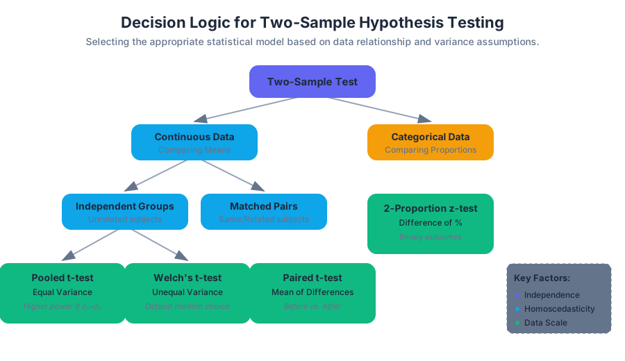
The Chi-Square Distribution: Foundations of Categorical Analysis

The Chi-Square ($\chi^2$) distribution is a continuous probability distribution that serves as the backbone for inferential statistics involving categorical data. While the Normal distribution governs the behavior of means, the Chi-Square distribution governs the behavior of variances and the "closeness" of observed data to theoretical models. It is not a single curve, but a family of curves defined by a single parameter: the degrees of freedom ($df$).

1. The Mathematical Foundation

At its most fundamental level, the Chi-Square distribution is derived from the Standard Normal Distribution ($Z \sim N(0,1)$). If you take a random variable from a standard normal distribution and square it, the resulting value follows a Chi-Square distribution with one degree of freedom.

Formal Definition: If $Z_1, Z_2, \dots, Z_k$ are independent, standard normal random variables, then the sum of their squares is distributed according to the Chi-Square distribution with $k$ degrees of freedom: $$X = \sum_{i=1}^{k} Z_i^2 \sim \chi^2(k)$$

Characteristics of the Distribution

The shape of the $\chi^2$ curve is highly sensitive to the value of $k$.

Property	Description	Mathematical Expression
Support	The distribution is defined only for non-negative values.	$[0, \infty)$
Mean	The expected value is exactly equal to the degrees of freedom.	$E[X] = k$
Variance	The spread is twice the degrees of freedom.	$Var(X) = 2k$
Skewness	Always right-skewed, but approaches normality as $k \to \infty$.	$\gamma_1 = \sqrt{8/k}$
Mode	The peak of the density function (for $k > 2$).	$k - 2$

As $df$ increases, the distribution loses its sharp right skew and begins to look like a bell curve. This is an application of the Central Limit Theorem, as the distribution is essentially a sum of independent random variables.

2. Goodness-of-Fit: Testing Theoretical Models

The Chi-Square Goodness-of-Fit Test is used to determine if a sample data set matches a population with a specific distribution. It answers the question: "Is the difference between what I saw and what I expected just due to chance?"

The Mechanics

The test relies on comparing Observed frequencies ($O$) from your sample against Expected frequencies ($E$) derived from your null hypothesis ($H_0$).

1. State the Hypotheses: $H_0$ states the data follows the specified distribution; $H_a$ states it does not.
2. Calculate Expected Values: $E = n \times p$, where $n$ is the total sample size and $p$ is the hypothesized probability for that category.
3. Compute the Test Statistic: $$\chi^2 = \sum \frac{(O_i - E_i)^2}{E_i}$$
4. Determine Degrees of Freedom: $df = k - 1$, where $k$ is the number of categories.

Low-Level Implementation (Python/NumPy)

To understand the mechanics, we can implement the calculation manually before relying on high-level libraries.

import numpy as np

def chi_square_gof(observed, expected_probs):
    """
    Manual implementation of the Chi-Square Goodness-of-Fit test.
    
    Args:
        observed (list): Raw counts for each category
        expected_probs (list): Hypothesized probabilities (must sum to 1)
    """
    obs = np.array(observed)
    n = obs.sum()
    exp = np.array(expected_probs) * n
    
    # The core Chi-Square formula: sum of squared residuals normalized by expectation
    chi_sq_stat = np.sum(np.square(obs - exp) / exp)
    
    # Degrees of freedom = categories - 1
    df = len(obs) - 1
    
    return chi_sq_stat, df

# Example: Testing if a 6-sided die is fair
# Observed counts for 600 rolls
rolls = [95, 105, 110, 90, 102, 98]
probs = [1/6] * 6

stat, df = chi_square_gof(rolls, probs)
print(f"Chi-Square Statistic: {stat:.4f}, DF: {df}")

3. The Test of Independence

While Goodness-of-Fit looks at one variable, the Test of Independence evaluates the relationship between two categorical variables. For example, is "Voting Preference" independent of "Income Level"?

Contingency Tables

Data for this test is organized into a Contingency Table (or cross-tabulation).

	Category A1	Category A2	Row Total
Category B1	Cell(1,1)	Cell(1,2)	$R_1$
Category B2	Cell(2,1)	Cell(2,2)	$R_2$
Col Total	$C_1$	$C_2$	Grand Total ($N$)

Calculating Expected Values in Independence Tests

In a test of independence, the expected value for any cell is calculated based on the assumption that the variables are independent (i.e., the joint probability is the product of the marginal probabilities).

Expected Cell Frequency Formula: $$E_{i,j} = \frac{(\text{Row } i \text{ Total}) \times (\text{Column } j \text{ Total})}{\text{Grand Total}}$$

Degrees of Freedom for Independence

For a table with $r$ rows and $c$ columns: $$df = (r - 1) \times (c - 1)$$ This represents the number of cells in the table that can vary independently given that the row and column totals are fixed.

Mathematical Derivation Logic

The following pseudocode outlines the logic used by statistical engines to process contingency tables.

ALGORITHM ChiSquareIndependence(Matrix Observed):
    Rows = Observed.RowCount
    Cols = Observed.ColCount
    GrandTotal = Sum(Observed)
    
    RowTotals = [Sum(Row) for Row in Observed]
    ColTotals = [Sum(Col) for Col in Observed.Columns]
    
    ChiSqStat = 0
    FOR i FROM 0 TO Rows-1:
        FOR j FROM 0 TO Cols-1:
            Expected = (RowTotals[i] * ColTotals[j]) / GrandTotal
            IF Expected < 5:
                WARN "Sample size too small for reliable Chi-Square"
            
            Residual = Observed[i][j] - Expected
            ChiSqStat += (Residual^2) / Expected
            
    DF = (Rows - 1) * (Cols - 1)
    PValue = 1 - ChiSquareCDF(ChiSqStat, DF)
    
    RETURN ChiSqStat, DF, PValue

4. Test of Homogeneity

The Test of Homogeneity is mathematically identical to the Test of Independence but differs in its experimental design and null hypothesis.

• Independence: You take one sample from one population and see if two variables are related.
• Homogeneity: You take samples from multiple distinct populations and see if they follow the same distribution for a single variable.

Feature	Test of Independence	Test of Homogeneity
Sampling	Single random sample	Multiple independent samples (one per population)
Question	Are Variable X and Variable Y related?	Is the distribution of Variable X the same across populations?
Null Hypothesis	Factors are independent.	Distributions are the same (homogeneous).
Calculation	$(r-1)(c-1)$	$(r-1)(c-1)$

5. Practical Implementation: Real-World Usage

In modern data science, we rarely calculate these by hand. We use libraries that handle the distribution's cumulative density function (CDF) to return p-values directly.

Library Call Example (SciPy)

This example demonstrates a test of independence between "Treatment Group" and "Recovery Status."

from scipy.stats import chi2_contingency

# Data: Rows = [Placebo, Drug A, Drug B]
# Columns = [Recovered, Not Recovered]
table = [
    [30, 70],  # Placebo
    [50, 50],  # Drug A
    [85, 15]   # Drug B
]

chi2, p, dof, expected = chi2_contingency(table)

print(f"P-value: {p:.10f}")
if p < 0.05:
    print("Reject H0: There is a significant relationship between treatment and recovery.")
else:
    print("Fail to reject H0: No significant relationship found.")

6. Critical Assumptions and Pitfalls

The Chi-Square test is a non-parametric test in terms of population distribution (it doesn't assume the population is normal), but it is parametric in its requirement for sample sizes.

The "Rule of Five"

The most common mistake in Chi-Square analysis is applying it to small datasets. Because the $\chi^2$ distribution is a continuous approximation of a discrete process, it breaks down when expected frequencies are low.

• Cochran’s Rule: No more than 20% of the expected counts should be less than 5, and all individual expected counts should be greater than 1.
• Yates' Correction: For $2 \times 2$ tables, some statisticians apply a "continuity correction" by subtracting 0.5 from the absolute difference between $O$ and $E$. However, modern consensus often favors the Fisher's Exact Test for small samples instead.

Comparison of Methods for Categorical Data

Method	Best Use Case	Constraint
Pearson's $\chi^2$	Large samples, any table size	$E_i \ge 5$
Fisher's Exact Test	$2 \times 2$ tables, small samples	Computationally expensive for large $N$
G-Test	Likelihood ratio based, additive	Preferred in bioinformatics/complex models
McNemar's Test	Paired categorical data (before/after)	Only for dependent samples

7. Advanced Variations: The Non-Central Chi-Square

In power analysis, we often encounter the Non-Central Chi-Square distribution. While the standard (central) Chi-Square assumes the null hypothesis is true, the non-central version describes the distribution of the test statistic when the alternative hypothesis is true.

It introduces a non-centrality parameter ($\lambda$): $$\lambda = \sum_{i=1}^{k} \mu_i^2$$ where $\mu_i$ are the means of the squared normal variables. This is crucial for calculating the Statistical Power (the probability of correctly rejecting a false null hypothesis).

8. Summary of Workflow

To perform a Chi-Square analysis effectively, follow this pipeline:

1. Identify the Test Type: Is it one variable vs. a model (GoF), two variables in one population (Independence), or one variable across multiple populations (Homogeneity)?
2. Verify Assumptions: Check that the data are frequencies (counts), observations are independent, and expected values are $\ge 5$.
3. Construct the Table: Ensure rows and columns are mutually exclusive.
4. Calculate $\chi^2$ and $df$: Use the sum of squared residuals.
5. Compare to Critical Value: Use a $\chi^2$ table or software to find the p-value for the given $df$ at the desired alpha level (usually 0.05).

Study Guide: The Chi-Square Distribution

Core Concepts

• Degrees of Freedom ($df$): The primary parameter of the $\chi^2$ distribution. For GoF, it's $k-1$. For Independence, it's $(r-1)(c-1)$.
• Observed vs. Expected: The test statistic measures the cumulative deviation of actual counts ($O$) from what we would expect under the null hypothesis ($E$).
• Right-Skewed Nature: The distribution starts at zero and has a long right tail. As $df$ increases, it becomes more symmetrical.

Common Formulas

• Test Statistic: $\chi^2 = \sum \frac{(O-E)^2}{E}$
• Expected (Independence): $E = \frac{\text{Row Total} \cdot \text{Col Total}}{N}$
• Mean of Distribution: $\mu = df$
• Variance of Distribution: $\sigma^2 = 2 \cdot df$

Critical Thinking Questions

1. Why can a Chi-Square statistic never be negative? (Answer: Because it is a sum of squared values).
2. What happens to the p-value if the gap between Observed and Expected values increases? (Answer: The $\chi^2$ statistic increases, causing the p-value to decrease).
3. If you have a $3 \times 4$ contingency table, what is the $df$? (Answer: $(3-1) \times (4-1) = 2 \times 3 = 6$).

Practical Tips

• Always use raw counts, never percentages or means, inside the Chi-Square formula.
• If your expected values are too low, consider "collapsing" categories (combining small groups) to meet the "Rule of Five."
• Remember that "Independence" does not mean "no relationship"—it specifically means no statistical association between the categorical groupings.

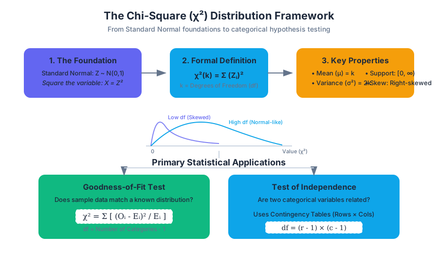
Linear Regression and Correlation

In the landscape of statistical modeling, the relationship between two quantitative variables serves as the bedrock for predictive analytics. Linear Regression and Correlation are the primary tools used to quantify the strength of these relationships and model the functional form they take. While correlation measures the degree of association, regression provides a mathematical framework to predict an outcome variable ($Y$) based on a predictor variable ($X$).

This article explores the mechanics of the Least-Squares Regression Line, the nuances of the Correlation Coefficient ($r$), the diagnostic power of Residuals, and the interpretative depth of the Coefficient of Determination ($r^2$).

---

The Correlation Coefficient ($r$)

The Pearson Product-Moment Correlation Coefficient, denoted as $r$, is a dimensionless index that quantifies the linear relationship between two variables. Developed by Karl Pearson, it measures both the direction (positive or negative) and the strength (magnitude) of the linear association.

What it is

Mathematically, $r$ is the ratio of the covariance of the two variables to the product of their standard deviations. This normalization ensures that $r$ always falls within the range of $[-1, 1]$.

Definition: Pearson's $r$ For a sample of $n$ paired observations $(x_i, y_i)$, the correlation coefficient is defined as: $$r = \frac{\sum_{i=1}^{n} (x_i - \bar{x})(y_i - \bar{y})}{\sqrt{\sum_{i=1}^{n} (x_i - \bar{x})^2 \sum_{i=1}^{n} (y_i - \bar{y})^2}}$$

Why it matters

Correlation allows researchers to determine if a relationship exists before attempting to build a predictive model. It is the first step in exploratory data analysis (EDA). However, it is vital to remember that correlation does not imply causation; it merely indicates that the variables move together in a linear fashion.

Interpretation of $r$ Values

The magnitude of $r$ dictates the "tightness" of the data points around a central line.

Value of $r$	Interpretation	Visual Characteristic
$r = 1$	Perfect Positive Correlation	All points lie exactly on a line with a positive slope.
$0.7 \le r < 1$	Strong Positive	Points are closely clustered around an upward-sloping line.
$0.3 \le r < 0.7$	Moderate Positive	A clear upward trend, but with significant dispersion.
$-0.3 < r < 0.3$	Weak or No Correlation	Points appear as a "cloud" with no discernible linear trend.
$r = -1$	Perfect Negative Correlation	All points lie exactly on a line with a negative slope.

Low-Level Implementation: Computing $r$ from Scratch

To understand the mechanics, we implement the calculation using raw NumPy, avoiding high-level library abstractions.

import numpy as np

def calculate_correlation(x, y):
    """
    Computes the Pearson Correlation Coefficient (r) using the 
    standard formula: cov(x, y) / (std(x) * std(y))
    """
    n = len(x)
    if n != len(y):
        raise ValueError("Arrays must be of equal length")

    # Calculate means
    mu_x, mu_y = np.mean(x), np.mean(y)

    # Calculate numerator: Sum of (x_i - mean_x) * (y_i - mean_y)
    numerator = np.sum((x - mu_x) * (y - mu_y))

    # Calculate denominator: sqrt(sum(x_i - mean_x)^2 * sum(y_i - mean_y)^2)
    sum_sq_diff_x = np.sum((x - mu_x)**2)
    sum_sq_diff_y = np.sum((y - mu_y)**2)
    denominator = np.sqrt(sum_sq_diff_x * sum_sq_diff_y)

    if denominator == 0:
        return 0  # Handle zero variance case
        
    return numerator / denominator

# Example usage
hours_studied = np.array([2, 3, 4, 5, 6])
exam_scores = np.array([65, 70, 75, 82, 89])
r_value = calculate_correlation(hours_studied, exam_scores)
print(f"Pearson Correlation (r): {r_value:.4f}")

---

Least-Squares Regression Line

While correlation tells us how well two variables relate, Linear Regression tells us how they relate. It defines the functional relationship as a straight line: $\hat{y} = a + bx$ (or $\hat{y} = \beta_0 + \beta_1 x$ in formal notation).

The Principle of Least Squares

The "best-fit" line is defined as the line that minimizes the Sum of Squared Errors (SSE). An error (or residual) is the vertical distance between an observed data point and the predicted point on the line. By squaring these distances, we ensure that positive and negative errors don't cancel out and that larger errors are penalized more heavily.

The Objective Function Minimize $SSE = \sum (y_i - \hat{y}_i)^2 = \sum (y_i - (a + bx_i))^2$

Deriving the Coefficients

The slope ($b$) and the intercept ($a$) are derived using calculus (setting partial derivatives to zero) or via the following standard formulas:

b = \frac{\sum (x_i - \bar{x})(y_i - \bar{y})}{\sum (x_i - \bar{x})^2} = r \left( \frac{s_y}{s_x} \right)

a = \bar{y} - b\bar{x}

Mathematical Representation: The Normal Equations

In matrix form, the solution for the coefficients $\beta$ is found by solving the "Normal Equations." This is the foundation for all modern linear modeling software.

Given the model: Y = Xβ + ε
The goal is to solve for β that minimizes ||Y - Xβ||²

The solution is:
β = (XᵀX)⁻¹ XᵀY

Where:
- X is the design matrix (with a column of 1s for the intercept)
- Xᵀ is the transpose of X
- (XᵀX)⁻¹ is the inverse of the product of X transpose and X
- Y is the vector of observed values

---

Coefficient of Determination ($r^2$)

The Coefficient of Determination, denoted as $r^2$, is perhaps the most vital metric for evaluating the performance of a regression model. It represents the proportion of the variance in the dependent variable that is predictable from the independent variable.

Partitioning Variance

To understand $r^2$, we must view the total variation in $Y$ as being composed of two parts: the variation explained by the model and the variation left over (unexplained).

Component	Symbol	Formula	Description
Total Sum of Squares	$SST$	$\sum (y_i - \bar{y})^2$	Total variation in the observed data.
Regression Sum of Squares	$SSR$	$\sum (\hat{y}_i - \bar{y})^2$	Variation explained by the linear relationship.
Error Sum of Squares	$SSE$	$\sum (y_i - \hat{y}_i)^2$	Unexplained variation (residuals).

The relationship between these is: $SST = SSR + SSE$. Therefore, $r^2$ is defined as: $$r^2 = \frac{SSR}{SST} = 1 - \frac{SSE}{SST}$$

Interpretation

If $r^2 = 0.85$, we say that 85% of the variation in $Y$ is explained by the linear relationship with $X$. The remaining 15% is attributed to other factors or inherent random noise.

---

Residual Analysis

A model is only as good as its assumptions. Residuals ($e_i = y_i - \hat{y}_i$) are the "leftovers" of the model. Analyzing residuals is the primary way we diagnose whether a linear model is appropriate for the data.

The LINE Assumptions

For a linear regression model to be valid for inference, four conditions must be met:

1. Linearity: The relationship between $X$ and $Y$ is linear.
2. Independence: Observations are independent of each other.
3. Normality: The residuals are normally distributed.
4. Equal Variance (Homoscedasticity): The variance of residuals is constant across all levels of $X$.

Diagnostic Plots

A Residual Plot (Residuals vs. $X$ or $\hat{y}$) should ideally look like a random "snowstorm" of points centered around zero.

• Curved Pattern: Suggests the relationship is non-linear (e.g., quadratic).
• Fan Shape (Heteroscedasticity): Suggests the error variance changes as $X$ increases, violating the equal variance assumption.
• Outliers: Points with large residuals that may disproportionately pull the regression line.

Real-World Usage: Scikit-Learn Pipeline

In professional environments, we use robust libraries to handle data scaling, model fitting, and metric calculation in a unified pipeline.

from sklearn.linear_model import LinearRegression
from sklearn.metrics import r2_score, mean_squared_error
import pandas as pd

# Load dataset
data = pd.DataFrame({
    'advertising_spend': [10, 20, 30, 40, 50, 60, 70, 80, 90, 100],
    'sales_revenue': [15, 28, 35, 52, 58, 72, 80, 95, 105, 120]
})

# Reshape for Scikit-Learn (expects 2D array for X)
X = data[['advertising_spend']]
y = data['sales_revenue']

# Initialize and fit model
model = LinearRegression()
model.fit(X, y)

# Predictions and Metrics
y_pred = model.predict(X)
r_squared = r2_score(y, y_pred)
mse = mean_squared_error(y, y_pred)

print(f"Model Slope (b): {model.coef_[0]:.2f}")
print(f"Model Intercept (a): {model.intercept_:.2f}")
print(f"R-squared: {r_squared:.4f}")
print(f"Mean Squared Error: {mse:.2f}")

---

Variations and Extensions

While simple linear regression involves one $X$ and one $Y$, the concept extends into several complex domains.

1. Multiple Linear Regression (MLR)

Predicting $Y$ using multiple independent variables: $\hat{y} = \beta_0 + \beta_1 x_1 + \beta_2 x_2 + ... + \beta_n x_n$. This allows for controlling confounding variables.

2. Non-linear Transformation

If the relationship is not linear, we can transform $X$ or $Y$ (e.g., $\log(x)$, $\sqrt{x}$, or $x^2$) to linearize the relationship before fitting the model.

3. Influential Points and Leverage

Not all data points are created equal.

• Outliers: Observations with extreme $Y$ values.
• High Leverage Points: Observations with extreme $X$ values.
• Influential Points: A point that, if removed, significantly changes the slope or intercept of the regression line.

Metric	Purpose	Threshold Idea
Cook's Distance	Measures influence of a single point.	Values > 1 often indicate high influence.
Standard Error ($s_e$)	Measures the average distance points fall from the line.	Smaller is better; used for confidence intervals.
p-value for Slope	Tests $H_0: \beta_1 = 0$.	If $p < 0.05$, the relationship is statistically significant.

---

Common Pitfalls and Misconceptions

1. Extrapolation

Predicting $Y$ values for $X$ values outside the range of the original data is dangerous. We have no evidence that the linear relationship continues indefinitely. For example, a model relating height to age in children cannot be extrapolated to predict the height of a 60-year-old.

2. Correlation $\neq$ Causation

A high $r$ value between "Ice Cream Sales" and "Drowning Incidents" does not mean ice cream causes drowning. Both are driven by a lurking variable: warm weather.

3. The Influence of Outliers

A single extreme outlier can inflate or deflate $r$ and significantly tilt the regression line, leading to a model that represents the outlier better than the bulk of the data.

4. Interpreting $r^2$ as Accuracy

$r^2$ measures "explained variance," not necessarily "accuracy." A model can have a high $r^2$ but still produce large prediction errors if the underlying variance of the data is high.

---

Practical Example: Real Estate Valuation

Imagine a dataset where $X$ is the square footage of a house and $Y$ is the sale price.

1. Correlation: We find $r = 0.92$, indicating a very strong positive relationship.
2. Regression: The line is $\hat{y} = 50,000 + 150x$.
   • The Intercept ($50,000$) suggests the base price of a lot before building.
   • The Slope ($150$) means for every additional square foot, the price increases by $\text{\textdollar}150$.
3. Coefficient of Determination: $r^2 = 0.846$. This means 84.6% of the price variation is explained by size. The other 15.4% might be due to location, age, or interior finishes.
4. Residuals: A house that sold for $\text{\textdollar}300,000$ but was predicted at $\text{\textdollar}280,000$ has a residual of $+\text{\textdollar}20,000$. This house was "overpriced" or had premium features not captured by square footage alone.

---

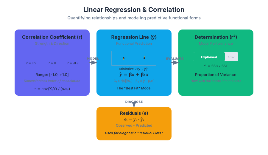
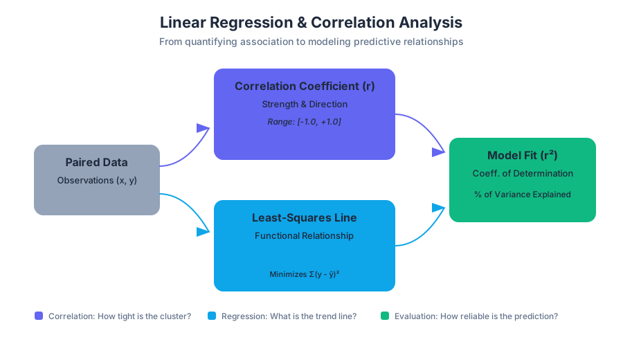
F Distribution and One-Way ANOVA

In the landscape of inferential statistics, the One-Way Analysis of Variance (ANOVA) stands as the primary gateway for comparing the means of three or more independent groups. While the Student’s t-test is sufficient for comparing two groups, its utility collapses under the weight of "Alpha Inflation" when applied to multiple comparisons. ANOVA sidesteps this by utilizing the F-Distribution to evaluate whether the observed variation between group means is significantly greater than the variation within those groups.

The Problem of Multiple Comparisons

Before diving into the mechanics of ANOVA, one must understand the motivation behind it. If a researcher wishes to compare five different medical treatments, they could theoretically perform ten separate t-tests to compare every possible pair. However, if each test has a significance level ($\alpha$) of 0.05, the probability of committing at least one Type I error (a false positive) across those ten tests is calculated as $1 - (1 - 0.05)^{10} \approx 0.40$.

This 40% "Family-wise Error Rate" is unacceptable. ANOVA solves this by performing a single "omnibus" test that maintains the $\alpha$ level at 0.05, regardless of the number of groups.

---

The F-Distribution: The Mathematical Engine

The F-Distribution is a continuous probability distribution that arises frequently as the null distribution of a test statistic, most notably in ANOVA. Unlike the symmetric Normal or T-distributions, the F-distribution is non-symmetric and governed by two distinct degrees of freedom.

Definition: The F-statistic is defined as the ratio of two independent chi-square ($\chi^2$) variables, each divided by its respective degrees of freedom. $$F = \frac{U_1 / d_1}{U_2 / d_2}$$ where $U_1$ and $U_2$ follow chi-square distributions with $d_1$ and $d_2$ degrees of freedom.

Characteristics of the F-Distribution

Property	Description
Skewness	Positively skewed (right-skewed), though it becomes more symmetric as degrees of freedom increase.
Range	$[0, \infty)$. Since it is a ratio of variances (which are squared), it can never be negative.
Parameters	Defined by $df_{num}$ (degrees of freedom for the numerator) and $df_{den}$ (degrees of freedom for the denominator).
Mean	For $df_{den} > 2$, the mean is $\frac{df_{den}}{df_{den} - 2}$. It is always slightly greater than 1.

---

One-Way ANOVA: Mechanics and Logic

The term "Analysis of Variance" is often a source of confusion for students. We are analyzing variances to make an inference about means. The core logic is a partition of the total variability in a dataset into two distinct components: the "Signal" (differences between groups) and the "Noise" (differences within groups).

The Variance Decomposition Identity

The fundamental identity of ANOVA is that the Total Sum of Squares (SST) can be decomposed into the Sum of Squares Between (SSB) and the Sum of Squares Within (SSW).

1. SST (Total Variation): The squared distance of every single data point from the "Grand Mean" (the average of all data points).
2. SSB (Between-Group Variation): The squared distance of each group's mean from the Grand Mean, weighted by the group size. This represents the effect of the independent variable.
3. SSW (Within-Group Variation): The squared distance of each data point from its own group's mean. This represents "error" or random chance.

The ANOVA Summary Table

This is the standard format for reporting results in academic papers and software outputs.

Source of Variation	Sum of Squares (SS)	Degrees of Freedom (df)	Mean Square (MS)	F-Ratio
Between (Factor)	$SSB$	$k - 1$	$MSB = \frac{SSB}{k-1}$	$F = \frac{MSB}{MSW}$
Within (Error)	$SSW$	$N - k$	$MSW = \frac{SSW}{N-k}$
Total	$SST$	$N - 1$

Where $k$ is the number of groups and $N$ is the total number of observations.

---

Low-Level Implementation: Calculating ANOVA from Scratch

To truly understand the F-statistic, one should see how the raw data is transformed into the ratio. The following Python implementation uses numpy to calculate the components without high-level statistical libraries.

import numpy as np

def perform_one_way_anova(*groups):
    """
    Performs a One-Way ANOVA on a variable number of groups.
    Returns: SSB, SSW, df_num, df_den, F_statistic
    """
    # Flatten all data to find the Grand Mean
    all_data = np.concatenate(groups)
    grand_mean = np.mean(all_data)
    N = len(all_data)
    k = len(groups)
    
    # 1. Calculate SSB (Between-Group Sum of Squares)
    ssb = 0
    for group in groups:
        n_j = len(group)
        group_mean = np.mean(group)
        ssb += n_j * (group_mean - grand_mean)**2
        
    # 2. Calculate SSW (Within-Group Sum of Squares)
    ssw = 0
    for group in groups:
        group_mean = np.mean(group)
        ssw += np.sum((group - group_mean)**2)
        
    # 3. Calculate Degrees of Freedom
    df_num = k - 1
    df_den = N - k
    
    # 4. Calculate Mean Squares
    msb = ssb / df_num
    msw = ssw / df_den
    
    # 5. Calculate F-statistic
    f_stat = msb / msw
    
    return {
        "F_stat": f_stat,
        "df_num": df_num,
        "df_den": df_den,
        "MSB": msb,
        "MSW": msw
    }

# Example Usage:
group_a = [12, 15, 14, 11, 13]
group_b = [20, 23, 21, 19, 22]
group_c = [15, 18, 17, 16, 19]

results = perform_one_way_anova(group_a, group_b, group_c)
print(f"F-Statistic: {results['F_stat']:.4f}")

---

Mathematical Derivation and the Null Hypothesis

The Null Hypothesis ($H_0$) for a One-Way ANOVA states that all group population means are equal: $$H_0: \mu_1 = \mu_2 = \mu_3 = \dots = \mu_k$$ The Alternative Hypothesis ($H_a$) states that at least one mean is different from the others.

The Logic of the F-Ratio

If $H_0$ is true, both $MSB$ and $MSW$ are independent estimates of the same population variance ($\sigma^2$). Therefore, their ratio should be approximately 1. If the treatment effect is large, $MSB$ will be significantly larger than $MSW$, pushing the F-statistic into the right tail of the distribution.

\begin{aligned}
\text{Total Sum of Squares (SST):} & \quad \sum_{i=1}^{k} \sum_{j=1}^{n_i} (X_{ij} - \bar{X}_{..})^2 \\
\text{Between Sum of Squares (SSB):} & \quad \sum_{i=1}^{k} n_i (\bar{X}_{i.} - \bar{X}_{..})^2 \\
\text{Within Sum of Squares (SSW):} & \quad \sum_{i=1}^{k} \sum_{j=1}^{n_i} (X_{ij} - \bar{X}_{i.})^2 \\
\text{F-Statistic:} & \quad F = \frac{SSB / (k-1)}{SSW / (n-k)}
\end{aligned}

---

Assumptions of One-Way ANOVA

For the F-test to be valid, the data must satisfy four critical assumptions. Violating these can lead to inflated Type I errors or a loss of statistical power.

Assumption	Explanation	Diagnostic Tool
Independence	Observations within and between groups must be independent.	Study design/Randomization
Normality	The dependent variable should be normally distributed within each group.	Shapiro-Wilk Test, Q-Q Plots
Homoscedasticity	Variances must be equal across all groups (Homogeneity of Variance).	Levene’s Test, Bartlett’s Test
Random Sampling	Data should be a random representative sample of the population.	Sampling Methodology

Note on Robustness: ANOVA is surprisingly robust to violations of normality, especially with large sample sizes. However, it is quite sensitive to unequal variances, particularly when group sizes are also unequal.

---

Post-Hoc Testing: "The Where"

If the ANOVA yields a significant p-value ($p < \alpha$), we reject the null hypothesis. However, the ANOVA does not tell us which specific groups are different. It only tells us that a difference exists somewhere. To find the specific differences, we use Post-Hoc Tests.

Common Post-Hoc Methods

1. Tukey’s HSD (Honest Significant Difference): The gold standard for comparing all possible pairs. It controls the family-wise error rate perfectly.
2. Bonferroni Correction: A conservative approach where you divide $\alpha$ by the number of comparisons.
3. Scheffé’s Method: Most flexible but least powerful; used for complex comparisons (e.g., comparing the average of groups A and B against group C).

High-Level Library Usage (R)

In professional practice, we rarely calculate these by hand. R provides a streamlined syntax for the entire pipeline.

# 1. Load data
data <- data.frame(
  score = c(12, 15, 14, 11, 13, 20, 23, 21, 19, 22, 15, 18, 17, 16, 19),
  group = factor(rep(c("A", "B", "C"), each = 5))
)

# 2. Run One-Way ANOVA
anova_model <- aov(score ~ group, data = data)

# 3. Check Summary
summary(anova_model)

# 4. If significant, run Tukey Post-Hoc
post_hoc <- TukeyHSD(anova_model)
print(post_hoc)

# 5. Visualize
plot(post_hoc)

---

Effect Size: Beyond P-Values

A significant p-value tells you that an effect exists, but it doesn't tell you how large the effect is. In ANOVA, we use Eta-squared ($\eta^2$) or Omega-squared ($\omega^2$).

• $\eta^2$: Calculated as $SSB / SST$. It represents the proportion of total variance explained by the factor.
• $\omega^2$: A less biased estimator, especially for small samples, as it accounts for degrees of freedom.

Effect Size ($\eta^2$)	Interpretation
~ 0.01	Small effect
~ 0.06	Medium effect
~ 0.14+	Large effect

---

Practical Application: A Clinical Example

Imagine a pharmaceutical company testing three dosages of a new blood pressure medication: 5mg, 10mg, and 20mg.

1. Data Collection: 30 patients are randomly assigned (10 per group).
2. Hypothesis: $H_0: \mu_{5} = \mu_{10} = \mu_{20}$.
3. ANOVA Execution: The software calculates an F-statistic of 5.42.
4. Critical Value: For $df(2, 27)$ and $\alpha = 0.05$, the critical F-value is 3.35.
5. Conclusion: Since $5.42 > 3.35$, we reject $H_0$. There is a significant difference in blood pressure reduction between dosages.
6. Post-Hoc: Tukey's HSD reveals that the 20mg dose is significantly better than 5mg, but the difference between 10mg and 20mg is not statistically significant.

---

Common Pitfalls and Misconceptions

• Mistaking the F-statistic for the P-value: The F-statistic is the test result; the p-value is the probability of seeing that result under the null hypothesis.
• Ignoring Outliers: A single extreme outlier can drastically inflate the $SSW$, making it impossible to find a significant $MSB/MSW$ ratio.
• Over-reliance on P-values: Always report effect sizes. In very large samples, even trivial differences become "statistically significant."
• Confusing One-Way with Two-Way ANOVA: One-Way ANOVA only looks at one independent variable (e.g., "Drug Type"). If you add a second variable (e.g., "Gender"), you must use a Two-Way ANOVA to account for interaction effects.

---

Data Engineering Perspective: ANOVA at Scale

In modern data pipelines, ANOVA is often used for feature selection or A/B/n testing. When dealing with millions of rows, calculating the Grand Mean and Sum of Squares can be done efficiently using SQL.

-- Calculating the components for ANOVA in a single pass
WITH GroupStats AS (
    SELECT 
        category,
        COUNT(*) as n_j,
        AVG(value) as group_mean,
        VAR_SAMP(value) * (COUNT(*) - 1) as group_ssw
    FROM experimental_results
    GROUP BY category
),
GrandStats AS (
    SELECT 
        SUM(n_j) as N,
        SUM(group_mean * n_j) / SUM(n_j) as grand_mean,
        SUM(group_ssw) as total_ssw
    FROM GroupStats
)
SELECT 
    (SUM(n_j * POWER(group_mean - grand_mean, 2))) / (COUNT(*) - 1) 
    / (total_ssw / (N - COUNT(*))) as f_statistic
FROM GroupStats, GrandStats;