Introductory Biology

Course Introduction and Biological Foundations

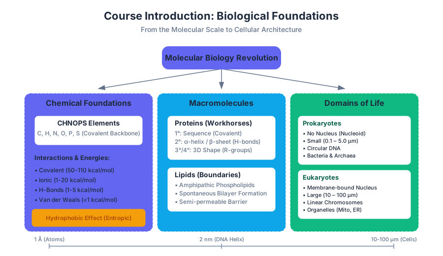
The study of biology has undergone a radical transformation over the last century, evolving from a purely descriptive discipline into a rigorous, molecular, and information-based science. This "Molecular Biology Revolution" has integrated principles from chemistry, physics, and engineering to decode the logic of living systems. At its core, modern biology seeks to understand how the interaction of inanimate molecules—lipids, proteins, nucleic acids, and carbohydrates—gives rise to the emergent property of life.

The Molecular Scale and Chemical Foundations

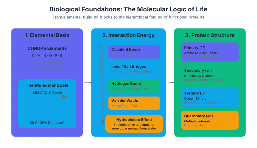
To understand biological systems, one must first appreciate the scale at which they operate. Biological interactions occur primarily at the nanometer ($10^{-9}$ m) and Angstrom ($\text{\AA}$, $10^{-10}$ m) scales. For context, a typical carbon-carbon covalent bond is approximately $1.54\ \text{\AA}$, while a DNA double helix is about $20\ \text{\AA}$ (2 nm) in diameter.

Life is built from a specific subset of the periodic table, often summarized by the acronym CHNOPS: Carbon, Hydrogen, Nitrogen, Oxygen, Phosphorus, and Sulfur. These elements form the covalent backbone of all biological macromolecules.

Covalent vs. Non-Covalent Interactions

The stability and dynamism of life depend on the balance between strong covalent bonds and weak non-covalent interactions.

• Covalent Bonds: Formed by the sharing of electron pairs. These are the "permanent" links that define the primary structure of molecules (e.g., the peptide bond in proteins).
• Non-Covalent Interactions: These are reversible and much weaker, yet they are responsible for the three-dimensional folding of proteins, the hybridization of DNA strands, and the formation of cell membranes.

Interaction Type	Typical Energy (kcal/mol)	Basis of Interaction	Biological Example
Covalent Bond	50 – 110	Electron sharing	Backbone of DNA
Ionic Interaction	1 – 20	Electrostatic attraction	Salt bridges in proteins
Hydrogen Bond	1 – 5	Dipole-dipole (H to O/N)	Base pairing in DNA
Van der Waals	< 1	Transient dipoles	Packing of lipid tails
Hydrophobic Effect	Variable (Entropic)	Exclusion of water	Protein core folding

The Hydrophobic Effect: This is perhaps the most important non-covalent "force" in biology. It is not an attractive force in the traditional sense, but an entropic drive. Water molecules form highly ordered "clathrate" cages around non-polar solutes. By sequestering non-polar groups together, the system minimizes the surface area in contact with water, releasing water molecules into the bulk phase and increasing the entropy of the universe ($\Delta S > 0$).

The Domains of Life and Cellular Architecture

Biological diversity is categorized into three primary domains: Bacteria, Archaea, and Eukarya. This classification is based on ribosomal RNA sequences and fundamental differences in cellular machinery.

Prokaryotes vs. Eukaryotes

The most significant structural divide is between prokaryotes (Bacteria and Archaea) and eukaryotes.

Feature	Prokaryotes	Eukaryotes
Nucleus	Absent (Nucleoid region)	Present (Membrane-bound)
Organelles	Generally absent	Present (Mitochondria, ER, Golgi)
DNA Structure	Circular, usually single	Linear, multiple chromosomes
Size	Small (0.1 – 5.0 $\mu$m)	Large (10 – 100 $\mu$m)
Transcription/Translation	Coupled in cytoplasm	Spatially separated
Cell Wall	Peptidoglycan (Bacteria)	Cellulose (Plants) or Chitin (Fungi)

Macromolecules I: Lipids and the Membrane Boundary

Lipids are unique among macromolecules because they are not polymers in the traditional sense. Instead, they aggregate through non-covalent interactions to form the phospholipid bilayer, which defines the boundary of the cell and its internal compartments.

Amphipathic Nature

A typical phospholipid consists of a hydrophilic (polar) "head" group and two hydrophobic (non-polar) fatty acid "tails." In an aqueous environment, these molecules spontaneously organize into bilayers.

• Self-Healing: Because the bilayer is held together by non-covalent hydrophobic interactions, it is dynamic. If the membrane is punctured, the hydrophobic tails' exposure to water is energetically unfavorable, causing the membrane to spontaneously reseal.
• Semi-permeability: The hydrophobic core acts as a barrier to ions and large polar molecules (e.g., $Na^+$, Glucose), while allowing small non-polar molecules (e.g., $O_2$, $CO_2$) to diffuse freely.

Macromolecules II: Proteins and Amino Acids

Proteins are the "workhorses" of the cell, serving as catalysts (enzymes), structural components, and signaling molecules. They are polymers of alpha-amino acids.

Amino Acid Structure

Every amino acid shares a common backbone: a central carbon ($\alpha$-carbon) bonded to an amino group ($-NH_2$), a carboxyl group ($-COOH$), a hydrogen atom, and a variable Side Chain (R-group). There are 20 standard amino acids, categorized by the chemical properties of their R-groups:

1. Non-polar (Hydrophobic): e.g., Leucine, Valine, Phenylalanine.
2. Polar Uncharged (Hydrophilic): e.g., Serine, Glutamine.
3. Charged: e.g., Aspartic Acid (negative), Lysine (positive).

Protein Folding and Hierarchy

Protein structure is described in four levels:

1. Primary ($1^\circ$): The linear sequence of amino acids linked by covalent peptide bonds.
2. Secondary ($2^\circ$): Local folding patterns like $\alpha$-helices and $\beta$-sheets, stabilized by hydrogen bonds between backbone atoms.
3. Tertiary ($3^\circ$): The overall 3D shape of a single polypeptide, driven by R-group interactions.
4. Quaternary ($4^\circ$): The assembly of multiple polypeptide subunits (e.g., Hemoglobin).

Case Study: Sickle Cell Anemia

Sickle cell anemia provides a classic example of how a microscopic change in primary structure yields a macroscopic disease state. A single point mutation in the gene for $\beta$-globin causes the substitution of Glutamic Acid (polar/charged) with Valine (non-polar) at position 6.

• Mechanism: In the deoxygenated state, the hydrophobic Valine residue on one hemoglobin molecule associates with a hydrophobic pocket on another. This leads to the polymerization of hemoglobin into long fibers, distorting the red blood cell into a "sickle" shape, which clogs capillaries and reduces oxygen transport.

# A simple script to calculate the Hydrophobicity Index of a protein sequence
# using the Kyte-Doolittle scale. High positive values = Hydrophobic.

kd_scale = {
    'A': 1.8, 'R': -4.5, 'N': -3.5, 'D': -3.5, 'C': 2.5,
    'Q': -3.5, 'E': -3.5, 'G': -0.4, 'H': -3.2, 'I': 4.5,
    'L': 3.8, 'K': -3.9, 'M': 1.9, 'F': 2.8, 'P': -1.6,
    'S': -0.8, 'T': -0.7, 'W': -0.9, 'Y': -1.3, 'V': 4.2
}

def calculate_hydrophobicity(sequence):
    """Calculates the average hydrophobicity of a given peptide string."""
    sequence = sequence.upper()
    try:
        scores = [kd_scale[amino_acid] for amino_acid in sequence]
        return sum(scores) / len(scores)
    except KeyError as e:
        return f"Invalid amino acid code: {e}"

# Example: Comparing a segment of Normal vs Sickle Cell Hemoglobin
normal_hb = "VHLTPEEKS" # Glu at pos 6
sickle_hb = "VHLTPVEKS" # Val at pos 6

print(f"Normal Hydrophobicity: {calculate_hydrophobicity(normal_hb):.2f}")
print(f"Sickle Hydrophobicity: {calculate_hydrophobicity(sickle_hb):.2f}")

Macromolecules III: Enzymes and Metabolism

Enzymes are biological catalysts that accelerate chemical reactions by lowering the Activation Energy ($E_a$). They do not change the equilibrium of a reaction ($\Delta G$), only the rate at which equilibrium is reached.

Thermodynamics of Life

Biological reactions are governed by the Gibbs Free Energy equation: $$\Delta G = \Delta H - T\Delta S$$

• Exergonic Reactions ($\Delta G < 0$): Spontaneous reactions that release energy.
• Endergonic Reactions ($\Delta G > 0$): Non-spontaneous reactions that require energy input.

Reaction Coupling: Cells perform endergonic reactions (like building DNA) by coupling them to highly exergonic reactions, most commonly the hydrolysis of ATP to ADP.

\begin{aligned}
\text{Reaction 1 (Endergonic): } & A \rightarrow B \quad (\Delta G = +5 \text{ kcal/mol}) \\
\text{Reaction 2 (Exergonic): } & ATP \rightarrow ADP + P_i \quad (\Delta G = -7.3 \text{ kcal/mol}) \\
\hline
\text{Coupled Reaction: } & A + ATP \rightarrow B + ADP + P_i \quad (\Delta G = -2.3 \text{ kcal/mol})
\end{aligned}

Macromolecules IV: Nucleic Acids and the Central Dogma

Nucleic acids (DNA and RNA) are the information-carrying molecules of the cell. They are polymers of nucleotides, each consisting of a sugar, a phosphate group, and a nitrogenous base (A, T, C, G, or U).

The Central Dogma

The Central Dogma describes the directional flow of genetic information:

1. Replication: DNA makes copies of itself.
2. Transcription: DNA is used as a template to synthesize messenger RNA (mRNA).
3. Translation: mRNA is read by ribosomes to synthesize a specific protein.

Gene Expression: While almost every cell in a multicellular organism contains the same genome, they look and function differently because they express different subsets of genes. This is regulated by transcription factors and epigenetic modifications.

# Bioinformatics Pipeline Example: 
# Using 'blastp' to find homologous protein sequences in a database

# 1. Create a BLAST database from a FASTA file of known proteins
makeblastdb -in proteins.fasta -dbtype prot -out human_proteome_db

# 2. Run a protein-protein BLAST search (blastp)
# -query: the sequence we want to search for
# -db: the database we just created
# -out: the output file
# -evalue: threshold for statistical significance (lower is better)
blastp -query unknown_sequence.fasta -db human_proteome_db -out results.txt -evalue 1e-5

# 3. Parse results to find the top hit
grep "Sequences producing significant alignments" -A 5 results.txt

Model Organisms in Biological Research

Because the fundamental mechanisms of life (the genetic code, metabolic pathways) are conserved across evolution, biologists use model organisms to study complex processes in simpler, more controllable systems.

Organism	Common Name	Primary Use
Escherichia coli	Bacteria	DNA replication, gene expression, protein production
Saccharomyces cerevisiae	Yeast	Eukaryotic cell cycle, protein trafficking
Arabidopsis thaliana	Thale cress	Plant genetics and development
Drosophila melanogaster	Fruit fly	Genetics, embryonic development
Caenorhabditis elegans	Roundworm	Cell lineage, apoptosis (cell death)
Mus musculus	Mouse	Immunology, human disease modeling

Common Pitfalls and Misconceptions

1. "Spontaneous" means "Fast": In thermodynamics, a spontaneous reaction ($\Delta G < 0$) is one that can occur without external energy, but it might take millions of years (e.g., the breakdown of a diamond). Enzymes are required to make these reactions occur on a biological timescale.
2. The "Blueprint" Metaphor: DNA is often called a blueprint, but it's more like a recipe or an executable program. A blueprint is a static 1:1 map; DNA contains conditional instructions (e.g., "if temperature > 37°C, produce Heat Shock Proteins").
3. Lipid Bilayer Rigidity: Students often imagine the cell membrane as a static wall. In reality, it is a "Fluid Mosaic." Lipids and proteins diffuse laterally within the plane of the membrane quite rapidly.

# Example of a Snakemake workflow configuration for a genomics pipeline
# This demonstrates the "Engineering" side of modern biology

samples:
  - "wildtype_rep1"
  - "mutant_rep1"

rule all:
    input:
        "results/final_report.html"

rule align_reads:
    input:
        fastq="data/{sample}.fastq",
        genome="ref/hg38.fa"
    output:
        bam="aligned/{sample}.bam"
    threads: 8
    shell:
        "bwa mem -t {threads} {input.genome} {input.fastq} | samtools view -Sb - > {output.bam}"

rule count_genes:
    input:
        bam="aligned/{sample}.bam",
        gtf="ref/hg38.gtf"
    output:
        counts="counts/{sample}.txt"
    shell:
        "featureCounts -a {input.gtf} -o {output.counts} {input.bam}"

Chemical Bonding and Biological Macromolecules

The Molecular Foundation of Life

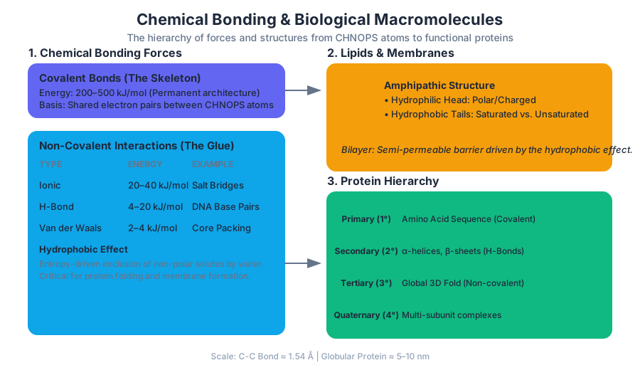
Biology has transitioned from a descriptive science of "what we see" to a precise engineering discipline of "how it works" at the molecular scale. To understand the cell, one must understand the forces governing the interactions of the CHNOPS elements (Carbon, Hydrogen, Nitrogen, Oxygen, Phosphorus, and Sulfur). These six elements constitute approximately 98% of the mass of most living organisms.

The scale of these interactions is measured in Angstroms ($\text{\AA}$, $10^{-10}$ m) and Nanometers (nm, $10^{-9}$ m). A typical C-C covalent bond is roughly $1.54\text{\AA}$, while the diameter of a globular protein may span 5–10 nm. At this scale, the distinction between "strong" and "weak" forces dictates the difference between a molecule's permanent architecture and its dynamic, functional movements.

Chemical Bonding: The Architecture of the Cell

Biological structures are held together by a continuum of forces, ranging from the robust sharing of electrons to transient induced dipoles.

Covalent Bonds: The "Hard-Wired" Skeleton

A covalent bond occurs when two atoms share a pair of valence electrons. In biological systems, these are the "permanent" connections that define the identity of a molecule.

• Bond Energy: Typically ranges from 200 to 500 kJ/mol. This is significantly higher than the thermal energy available at physiological temperature ($RT \approx 2.5$ kJ/mol), meaning covalent bonds do not break spontaneously.
• Polarity: When electrons are shared unequally due to differences in electronegativity (e.g., O-H or N-H bonds), the bond becomes polar, creating partial charges ($\delta+$ and $\delta-$) that are crucial for non-covalent interactions.

Non-Covalent Interactions: The Dynamic Glue

While covalent bonds build the molecules, non-covalent interactions determine how those molecules fold, associate, and signal.

Interaction Type	Basis of Interaction	Energy (kJ/mol)	Biological Example
Ionic Bond	Attraction between opposite full charges	20–40	Salt bridges in protein interiors
Hydrogen Bond	Dipole-dipole interaction involving H and O, N, or F	4–20	DNA base pairing; $\alpha$-helices
Van der Waals	Transient induced dipoles	2–4	Packing of non-polar side chains
Hydrophobic Effect	Entropy-driven exclusion of non-polar solutes	Variable	Protein folding; Membrane formation

The Hydrophobic Effect

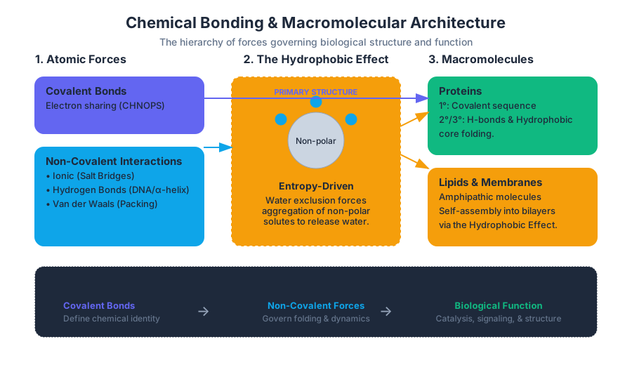
The hydrophobic effect is perhaps the most misunderstood "force" in biology. It is not an attractive force between non-polar molecules, but rather an entropy-driven exclusion of non-polar substances by water.

Definition: When a non-polar molecule is placed in water, the water molecules are forced to form a highly ordered "clathrate" cage around it to maintain hydrogen bonding. This decrease in the entropy of water ($\Delta S < 0$) is energetically unfavorable. By aggregating together, non-polar molecules minimize their surface area, releasing water molecules back into the bulk phase and increasing the total entropy of the system ($\Delta S > 0$).

Lipids and Biological Membranes

Lipids are unique among the four macromolecule classes because they are not polymers in the traditional sense. Instead, they are defined by their solubility: they are hydrophobic or amphipathic (possessing both hydrophilic and hydrophobic regions).

Phospholipids and the Bilayer

The fundamental unit of the cell membrane is the phospholipid. It consists of a glycerol backbone, two fatty acid "tails," and a phosphate-containing "head" group.

1. The Head: Polar and hydrophilic, interacting with the aqueous environment.
2. The Tails: Non-polar hydrocarbon chains.
   • Saturated: No double bonds; straight chains that pack tightly (solid at room temp).
   • Unsaturated: Contain one or more cis-double bonds; "kinks" prevent tight packing (liquid at room temp).

Membrane Dynamics and Permeability

The lipid bilayer is a semi-permeable barrier. It allows the passage of small, non-polar molecules (like $O_2$ and $CO_2$) but acts as a formidable barrier to ions and large polar molecules (like glucose).

/* 
 * A low-level simulation snippet for calculating 
 * the Lennard-Jones potential between two lipid tail atoms.
 * V_lj = 4 * epsilon * [(sigma/r)^12 - (sigma/r)^6]
 */

#include <math.h>
#include <stdio.h>

typedef struct {
    double x, y, z;
} Atom;

double calculate_vdw_energy(Atom a, Atom b, double epsilon, double sigma) {
    double dx = a.x - b.x;
    double dy = a.y - b.y;
    double dz = a.z - b.z;
    double r2 = dx*dx + dy*dy + dz*dz;
    double r6 = r2 * r2 * r2;
    double r12 = r6 * r6;
    
    double sigma6 = pow(sigma, 6);
    double sigma12 = sigma6 * sigma6;
    
    return 4.0 * epsilon * (sigma12/r12 - sigma6/r6);
}

Protein Hierarchy: From Sequence to Function

Proteins are the "workhorses" of the cell, executing the instructions encoded in DNA. They are polymers of $\alpha$-amino acids.

The Amino Acid Building Block

Every amino acid shares a common structure: a central carbon ($C_\alpha$), an amino group ($-NH_2$), a carboxyl group ($-COOH$), and a variable R-group (side chain). There are 20 standard amino acids, categorized by the chemical nature of their R-groups.

Category	Properties	Examples
Non-polar	Hydrophobic; found in protein cores	Leucine, Valine, Phenylalanine
Polar Uncharged	Can form H-bonds; hydrophilic	Serine, Threonine, Glutamine
Charged (Acidic)	Negatively charged at pH 7	Aspartic Acid, Glutamic Acid
Charged (Basic)	Positively charged at pH 7	Lysine, Arginine, Histidine

The Four Levels of Protein Structure

1. Primary ($1^\circ$): The linear sequence of amino acids linked by peptide bonds. The peptide bond has double-bond character due to resonance, making it planar and rigid.
2. Secondary ($2^\circ$): Local spatial arrangement of the backbone, stabilized by H-bonds between the backbone carbonyl oxygen and amide hydrogen. Common motifs include the $\alpha$-helix and $\beta$-pleated sheet.
3. Tertiary ($3^\circ$): The overall 3D fold of a single polypeptide chain, driven by R-group interactions (hydrophobic packing, ionic bridges, disulfide bonds).
4. Quaternary ($4^\circ$): The association of multiple polypeptide subunits into a functional complex (e.g., the four subunits of Hemoglobin).

Case Study: Sickle Cell Anemia

Sickle cell anemia is a profound example of how a change in the $1^\circ$ sequence dictates $4^\circ$ pathology. A single mutation (Glu6 $\rightarrow$ Val6) in the $\beta$-globin chain replaces a polar, charged residue with a non-polar, hydrophobic one. Under low oxygen conditions, this "hydrophobic patch" causes hemoglobin tetramers to polymerize into long fibers, distorting the red blood cell into a sickle shape.

\text{Gibbs Free Energy of Folding:} \\
\Delta G_{folding} = \Delta H_{folding} - T \Delta S_{folding} \\
\\
\text{Where:} \\
\Delta H \text{ (Enthalpy): Sum of H-bonds and VdW interactions.} \\
\Delta S \text{ (Entropy): Includes conformational entropy (negative) } \\
\text{and the hydrophobic effect (positive).}

Carbohydrates: Energy and Identity

Carbohydrates (saccharides) serve two primary roles: fuel storage and structural/recognition markers.

Monosaccharides and the Glycosidic Bond

Monosaccharides like glucose ($C_6H_{12}O_6$) can exist in linear or ring forms. When two monosaccharides link, they form a glycosidic bond via a dehydration reaction.

• $\alpha$-Linkage: The -OH group on Carbon-1 is below the plane. Found in Starch and Glycogen (easily digested for energy).
• $\beta$-Linkage: The -OH group on Carbon-1 is above the plane. Found in Cellulose (highly stable, structural component of plant cell walls). Humans lack the enzymes to hydrolyze $\beta$-1,4 linkages.

Glycoproteins and Blood Groups

Carbohydrates often conjugate to proteins (glycoproteins) on the cell surface. These "sugar coats" are essential for cell-cell recognition. The ABO blood group system is defined by specific carbohydrate antigens attached to lipids and proteins on the red blood cell surface.

Blood Type	Terminal Sugar	Enzyme Present
O	H-antigen (fucose)	None (functional)
A	N-acetylgalactosamine	A-transferase
B	Galactose	B-transferase
AB	Both A and B sugars	Both transferases

Common Pitfalls and Misconceptions

• The "Bond" Misnomer: Students often think of the "hydrophobic bond." There is no such thing. It is an exclusion principle driven by the entropy of water, not an attraction between lipids.
• Equilibrium vs. Rate: Enzymes (proteins) change the rate of a reaction by lowering activation energy ($E_a$), but they do not change the equilibrium constant ($K_{eq}$) or the $\Delta G$ of the reaction.
• Denaturation: Heating a protein breaks non-covalent interactions (secondary, tertiary, and quaternary structure) but usually leaves the covalent peptide bonds (primary structure) intact.

# Real-world usage: Calculating the Hydrophobicity Profile (Kyte-Doolittle)
# of a protein sequence to predict transmembrane domains.

def calculate_hydrophobicity(sequence, window_size=19):
    kd_scale = {
        'A': 1.8, 'R': -4.5, 'N': -3.5, 'D': -3.5, 'C': 2.5,
        'Q': -3.5, 'E': -3.5, 'G': -0.4, 'H': -3.2, 'I': 4.5,
        'L': 3.8, 'K': -3.9, 'M': 1.9, 'F': 2.8, 'P': -1.6,
        'S': -0.8, 'T': -0.7, 'W': -0.9, 'Y': -1.3, 'V': 4.2
    }
    
    scores = []
    for i in range(len(sequence) - window_size + 1):
        window = sequence[i : i + window_size]
        score = sum(kd_scale.get(aa, 0) for aa in window) / window_size
        scores.append(round(score, 2))
    
    return scores

# Example: A segment of Bacteriorhodopsin (a transmembrane protein)
seq = "GVAFITILLGVLLVGF"
print(f"Hydrophobicity Profile: {calculate_hydrophobicity(seq, window_size=5)}")

Enzyme Kinetics and Thermodynamics

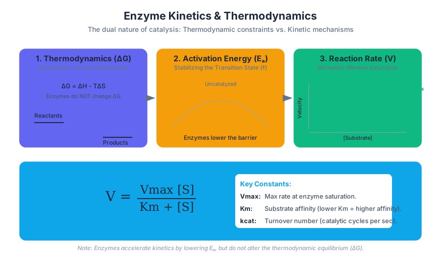
Enzymes are the sophisticated molecular machines that underpin all biological life. While a simple chemical reaction might take centuries to occur spontaneously, an enzyme can accelerate that same process by factors of $10^6$ to $10^{12}$. This section explores the dual nature of enzymatic catalysis: the thermodynamic constraints that dictate whether a reaction can happen, and the kinetic mechanisms that determine how fast it actually occurs.

The Thermodynamic Landscape: Free Energy (ΔG)

In biological systems, the "possibility" of a reaction is governed by the laws of thermodynamics. Specifically, we look at the Gibbs Free Energy (ΔG), which represents the energy available to do work at constant temperature and pressure.

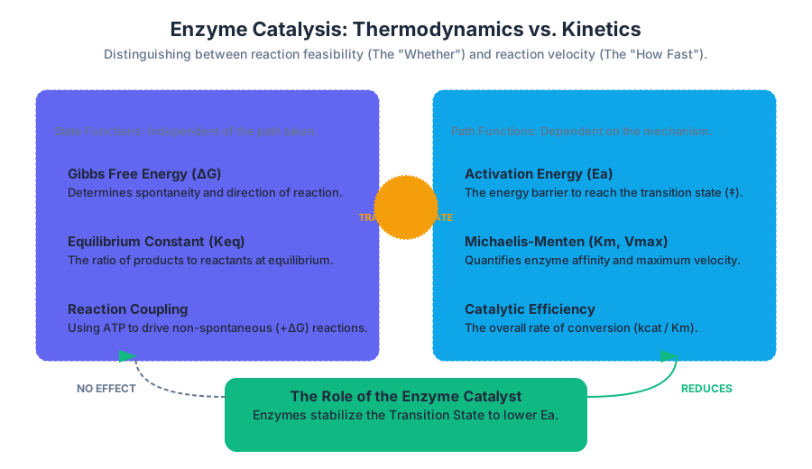
The First Law of Bio-Thermodynamics: Enzymes do not, and cannot, alter the equilibrium constant ($K_{eq}$) or the total free energy change ($\Delta G$) of a reaction. They only change the path taken to reach that equilibrium.

Gibbs Free Energy and Spontaneity

The relationship between enthalpy ($\Delta H$), entropy ($\Delta S$), and temperature ($T$) is defined by the equation: $$\Delta G = \Delta H - T\Delta S$$

A reaction is exergonic (spontaneous) if $\Delta G < 0$ and endergonic (non-spontaneous) if $\Delta G > 0$. In the context of metabolic pathways, cells often perform endergonic reactions by reaction coupling—linking a non-spontaneous reaction to a highly spontaneous one, such as the hydrolysis of ATP.

Parameter	Symbol	Definition	Impact on Spontaneity
Gibbs Free Energy	$\Delta G$	Total energy available for work	Negative value indicates spontaneity.
Enthalpy	$\Delta H$	Total heat content of the system	Exothermic ($\Delta H < 0$) favors spontaneity.
Entropy	$\Delta S$	Degree of disorder/randomness	Increase ($\Delta S > 0$) favors spontaneity.
Standard Free Energy	$\Delta G^{\circ'}$	$\Delta G$ at pH 7, 25°C, 1M concentration	Benchmarking constant for biochemical reactions.

Reaction Coupling and Flux

In a metabolic pathway, the overall $\Delta G$ is the sum of the individual steps. This allows a cell to "pull" a reaction forward even if a specific intermediate step is slightly unfavorable, provided the subsequent step is highly favorable (a concept known as metabolic flux).

Activation Energy and the Transition State

If a reaction is exergonic, why doesn't it happen instantly? The answer lies in the Activation Energy ($E_a$). Even if the products are at a lower energy state than the reactants, the system must first pass through a high-energy, unstable configuration known as the Transition State (‡).

How Enzymes Lower $E_a$

Enzymes function by stabilizing this transition state. By providing an environment (the active site) that is chemically complementary to the transition state, the enzyme reduces the energy "hump" the reactants must climb.

1. Proximity and Orientation: The enzyme holds substrates in the exact geometry required for the reaction to occur.
2. Microenvironment: The active site may exclude water, change local pH, or provide metal ion cofactors to facilitate electron transfer.
3. Induced Fit: As the substrate binds, the enzyme undergoes a conformational change that strains the substrate’s bonds, pushing it toward the transition state.

Mathematical Representation of Reaction Rates

The relationship between the rate constant ($k$) and activation energy is described by the Arrhenius Equation: $$k = Ae^{-E_a / RT}$$ Where $A$ is the frequency factor, $R$ is the gas constant, and $T$ is temperature. Because $E_a$ is in the exponent, even a small reduction in activation energy results in a massive increase in the reaction rate.

Michaelis-Menten Kinetics

To quantify how well an enzyme works, we use the Michaelis-Menten model. This model assumes a simple two-step process: the formation of an Enzyme-Substrate (ES) complex, followed by the catalytic step that releases the product (P).

$$E + S \xrightarrow{k_1, k_{-1}} ES \xrightarrow{k_{cat}} E + P$$

The Michaelis-Menten Equation

The fundamental equation relating reaction velocity ($V$) to substrate concentration $[S]$ is: $$V = \frac{V_{max}[S]}{K_m + [S]}$$

Constant	Name	Meaning
$V_{max}$	Maximum Velocity	The rate when the enzyme is fully saturated with substrate.
$K_m$	Michaelis Constant	The $[S]$ at which $V = 1/2 V_{max}$; inversely related to substrate affinity.
$k_{cat}$	Turnover Number	Number of substrate molecules converted to product per unit time per enzyme.
$k_{cat}/K_m$	Catalytic Efficiency	The "perfection" of the enzyme; limited by the rate of diffusion.

Derivation and Implementation

In a computational context, we often need to simulate these kinetics to predict metabolic behavior or fit experimental data.

import numpy as np
import matplotlib.pyplot as plt
from scipy.optimize import curve_fit

def michaelis_menten(s, v_max, k_m):
    """
    Standard Michaelis-Menten model for enzyme kinetics.
    s: substrate concentration
    v_max: maximum reaction velocity
    k_m: Michaelis constant (affinity)
    """
    return (v_max * s) / (k_m + s)

# Simulated experimental data (Substrate concentration in mM, Velocity in umol/min)
s_data = np.array([0.5, 1.0, 2.0, 5.0, 10.0, 20.0])
v_data = np.array([12.1, 21.5, 33.8, 52.1, 65.4, 74.2])

# Perform non-linear least squares fit
params, covariance = curve_fit(michaelis_menten, s_data, v_data)
v_max_fit, k_m_fit = params

print(f"Calculated Vmax: {v_max_fit:.2f}")
print(f"Calculated Km: {k_m_fit:.2f}")

# Visualization
s_smooth = np.linspace(0, 25, 100)
plt.scatter(s_data, v_data, label='Experimental Data')
plt.plot(s_smooth, michaelis_menten(s_smooth, v_max_fit, k_m_fit), 'r-', label='Fit')
plt.xlabel('[S] (mM)')
plt.ylabel('Velocity (V)')
plt.legend()
plt.show()

Enzyme Inhibition: Modulating Activity

Inhibition is the primary mechanism for drug action and cellular regulation. Inhibitors are molecules that decrease the rate of an enzymatic reaction. They are classified based on where they bind and how they affect the kinetic parameters $V_{max}$ and $K_m$.

Types of Inhibition

1. Competitive Inhibition: The inhibitor resembles the substrate and competes for the active site. Increasing $[S]$ can overcome this inhibition.
   • Effect: $V_{max}$ stays the same; $K_m$ increases.
2. Uncompetitive Inhibition: The inhibitor binds only to the Enzyme-Substrate (ES) complex. It "locks" the substrate in, preventing the reaction.
   • Effect: Both $V_{max}$ and $K_m$ decrease.
3. Non-competitive (Mixed) Inhibition: The inhibitor binds to an allosteric site (not the active site), regardless of whether the substrate is bound.
   • Effect: $V_{max}$ decreases; $K_m$ usually stays the same (in pure non-competitive).

The Lineweaver-Burk Plot

To distinguish between these types of inhibition, scientists use the double-reciprocal plot. By taking the reciprocal of the Michaelis-Menten equation, we get a linear form: $$\frac{1}{V} = \frac{K_m}{V_{max}} \cdot \frac{1}{[S]} + \frac{1}{V_{max}}$$

\begin{aligned}
&\text{Lineweaver-Burk Analysis:} \\
&\text{y-intercept} = 1/V_{max} \\
&\text{x-intercept} = -1/K_m \\
&\text{slope} = K_m/V_{max}
\end{aligned}

Inhibition Type	$V_{max}$ Change	$K_m$ Change	Lineweaver-Burk Intersection
Competitive	Unchanged	Increases	Intersect at Y-axis ($1/V_{max}$)
Uncompetitive	Decreases	Decreases	Parallel lines (Slope unchanged)
Non-competitive	Decreases	Unchanged	Intersect at X-axis ($-1/K_m$)

Allosteric Regulation and Cooperativity

Not all enzymes follow Michaelis-Menten kinetics. Many regulatory enzymes exhibit allosteric regulation, where the binding of a molecule at one site affects the binding of a molecule at a distant site.

Sigmoidal Kinetics

Allosteric enzymes often show a sigmoidal (S-shaped) curve rather than a hyperbolic one. This indicates cooperativity. In positive cooperativity, the binding of the first substrate molecule makes it easier for subsequent molecules to bind. This allows the enzyme to act as a "switch," being highly sensitive to small changes in substrate concentration within a narrow range.

The Hill Equation

Cooperativity is quantified using the Hill coefficient ($n$): $$V = \frac{V_{max}[S]^n}{K_{0.5}^n + [S]^n}$$

• $n > 1$: Positive cooperativity (e.g., Hemoglobin binding Oxygen).
• $n = 1$: Non-cooperative (Michaelis-Menten).
• $n < 1$: Negative cooperativity.

Key Insight: Allosteric effectors can be activators or inhibitors. They shift the sigmoidal curve to the left (activation, lower $K_{0.5}$) or to the right (inhibition, higher $K_{0.5}$), allowing for precise "fine-tuning" of metabolic flux.

Metabolic Pathways and Feedback Loops

Enzymes rarely act in isolation. They are organized into metabolic pathways where the product of one enzyme becomes the substrate for the next.

Feedback Inhibition (End-Product Inhibition)

To maintain homeostasis, the final product of a pathway often acts as an allosteric inhibitor of the first "committed step" in that pathway. This prevents the wasteful overproduction of metabolites.

Example: Phenylketonuria (PKU)

A classic example of metabolic failure is Phenylketonuria. The enzyme phenylalanine hydroxylase (PAH) is responsible for converting the amino acid phenylalanine into tyrosine.

• The Defect: A mutation in the PAH gene leads to a non-functional enzyme.
• The Consequence: Phenylalanine builds up to toxic levels (hyperphenylalaninemia), leading to intellectual disability if not managed by diet.
• The Lesson: This illustrates the importance of enzyme "throughput." If one "pipe" in the metabolic plumbing is blocked, the entire system backs up, leading to pathological states.

Analyzing Pathway Flux with CLI Tools

Bioinformaticians often use tools like COBRApy (Constraint-Based Reconstruction and Analysis) to model these pathways at a genome scale.

# Example: Using a CLI tool to inspect a metabolic model (pseudocode/tool usage)
# 1. Load the model for E. coli (e.g., iML1515)
# 2. Set constraints (e.g., glucose uptake rate)
# 3. Optimize for biomass production (Growth)

cobra-cli model optimize --input iML1515.json --objective biomass_reaction

# Output might look like:
# Objective Value: 0.874 (Growth Rate hr^-1)
# Flux through Phenylalanine Hydroxylase: 0.042 mmol/gDCW/hr

Common Pitfalls in Kinetic Analysis

Even experienced researchers can stumble when interpreting enzyme data. Here are the most common traps:

• Ignoring pH and Temperature: Enzymes have narrow optima. A $V_{max}$ measured at pH 7.4 might be zero at pH 5.0 due to the protonation of critical active-site residues (like Histidine).
• Assuming $K_m$ is a Dissociation Constant ($K_d$): $K_m = (k_{-1} + k_{cat}) / k_1$. It only equals $K_d$ if $k_{cat}$ is much smaller than $k_{-1}$. In many efficient enzymes, this is not the case.
• Substrate Depletion: Michaelis-Menten assumes the "Initial Velocity" ($V_0$). If you let the reaction run too long, the substrate concentration drops, and the rate slows down naturally, leading to an underestimation of $V_{max}$.
• Non-Specific Inhibition: Some compounds inhibit enzymes by simply denaturing them or forming aggregates (detergent-like effects) rather than binding the active site.

DNA Structure and Replication

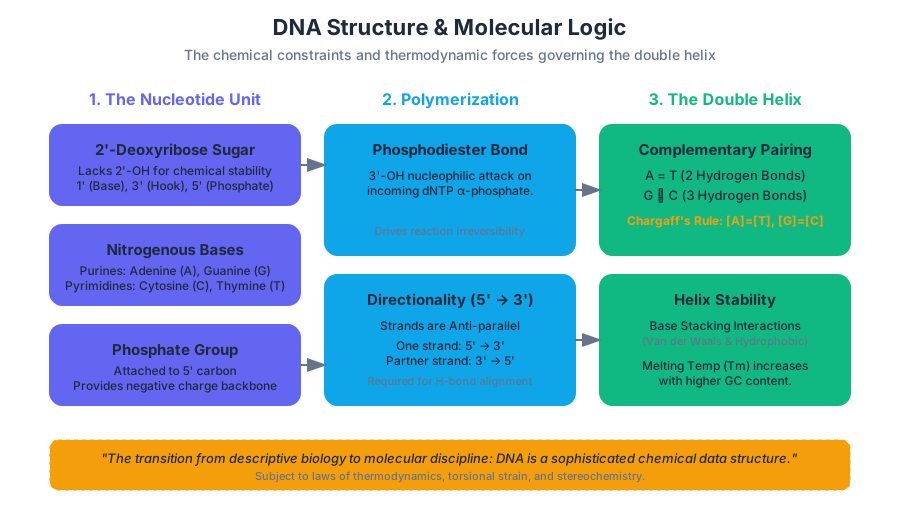
The transition of biology from a purely descriptive science to a rigorous molecular discipline is nowhere more evident than in the study of deoxyribonucleic acid (DNA). As we move from the macroscopic observations of Mendelian genetics to the nanometer-scale interactions of CHNOPS (Carbon, Hydrogen, Nitrogen, Oxygen, Phosphorus, and Sulfur), we find that life’s "blueprint" is not merely a metaphor, but a sophisticated chemical data structure.

In this deep dive, we examine the structural constraints of the double helix and the enzymatic choreography required to replicate three billion base pairs with near-perfect fidelity. We will treat the genome not just as a sequence of letters, but as a physical polymer subject to the laws of thermodynamics, torsional strain, and stereochemistry.

Nucleotide Structure: The Monomeric Unit

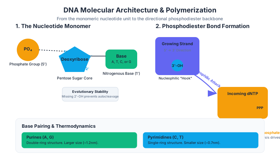
The fundamental building block of the nucleic acid is the nucleotide. To understand DNA, one must first master the anatomy of this monomer. A nucleotide consists of three distinct components: a pentose sugar, a nitrogenous base, and at least one phosphate group.

The Pentose Sugar: Deoxyribose

In DNA, the sugar is 2'-deoxyribose. The numbering of the carbons (1' through 5') is critical for understanding directionality.

• The 1' carbon is the attachment point for the nitrogenous base (via an N-glycosidic bond).
• The 2' carbon is "deoxy" in DNA, meaning it lacks the hydroxyl (-OH) group found in RNA. This single oxygen atom difference is a major evolutionary pivot; the absence of the 2'-OH makes DNA significantly more chemically stable than RNA, as it prevents auto-catalytic cleavage of the phosphodiester backbone.
• The 3' carbon bears a hydroxyl group, which serves as the "hook" for the next nucleotide.
• The 5' carbon is attached to the phosphate group.

Nitrogenous Bases: Purines and Pyrimidines

The "information" in DNA is encoded in the sequence of four nitrogenous bases. These are categorized by their ring structures:

Feature	Purines	Pyrimidines
Bases	Adenine (A), Guanine (G)	Cytosine (C), Thymine (T)
Structure	Double-ring (6-membered + 5-membered)	Single-ring (6-membered)
Size	Larger (~1.2 nm)	Smaller (~0.7 nm)
Hydrogen Bond Donors/Acceptors	A: 2 bonds; G: 3 bonds	T: 2 bonds; C: 3 bonds

The Chargaff Equivalence: In any double-stranded DNA molecule, the amount of A equals T, and the amount of G equals C. This is a direct consequence of the base-pairing requirements dictated by the hydrogen-bonding patterns within the helix.

The Phosphodiester Bond and Directionality

Nucleotides are polymerized into long chains via phosphodiester bonds. This is a covalent linkage where a phosphate group bridges the 5' carbon of one sugar to the 3' carbon of the next.

The Polymerization Mechanism

The synthesis of DNA is an endergonic process driven by the hydrolysis of high-energy nucleoside triphosphates (dNTPs). When a new nucleotide is added, the 3'-OH group of the existing strand performs a nucleophilic attack on the $\alpha$-phosphate of the incoming dNTP. This releases a pyrophosphate (PPi) molecule, which is subsequently hydrolyzed into two inorganic phosphates ($2P_i$). This secondary hydrolysis provides the thermodynamic "push" to make the overall reaction irreversible under cellular conditions.

Anti-parallel Orientation

A DNA double helix consists of two strands running in opposite directions. One strand runs 5' $\rightarrow$ 3', while its partner runs 3' $\rightarrow$ 5'. This anti-parallel nature is not an accident of geometry but a requirement for the hydrogen bonds between bases to align correctly.

# A low-level representation of DNA strand polarity and base pairing
class Nucleotide:
    def __init__(self, base, sugar="Deoxyribose"):
        self.base = base
        self.sugar = sugar
        self.upstream = None   # 5' connection
        self.downstream = None # 3' connection

class DNAStrand:
    def __init__(self, sequence):
        self.head = None
        self.tail = None
        self._build(sequence)

    def _build(self, sequence):
        for char in sequence:
            new_node = Nucleotide(char)
            if not self.head:
                self.head = new_node
            else:
                self.tail.downstream = new_node
                new_node.upstream = self.tail
            self.tail = new_node

    def get_complement(self):
        mapping = {'A': 'T', 'T': 'A', 'C': 'G', 'G': 'C'}
        # Complement must be reversed to represent 5'->3' convention
        comp_seq = "".join([mapping[n.base] for n in self._iterate_nodes()])[::-1]
        return comp_seq

    def _iterate_nodes(self):
        curr = self.head
        while curr:
            yield curr
            curr = curr.downstream

Thermodynamics of the Double Helix

The stability of the DNA helix is governed by two primary forces: Hydrogen Bonding between bases and Base Stacking interactions (van der Waals and hydrophobic effects) between the planar faces of the bases.

Melting Temperature ($T_m$)

The $T_m$ is the temperature at which 50% of the DNA molecules in a solution are denatured (separated into single strands). Because G-C pairs share three hydrogen bonds while A-T pairs share only two, DNA with a higher GC content is more thermally stable.

The $T_m$ can be approximated using the Wallace Rule for short oligonucleotides or the more robust nearest-neighbor thermodynamic model for longer sequences.

T_m = \frac{\Delta H}{\Delta S + R \ln(C/4)} - 273.15

Where:

• $\Delta H$: Enthalpy of hybridization
• $\Delta S$: Entropy of hybridization
• $R$: Ideal gas constant
• $C$: Concentration of the DNA

Interaction	$\Delta H$ (kcal/mol)	$\Delta S$ (cal/mol·K)
AA/TT	-7.9	-22.2
AT/TA	-7.2	-20.4
GC/CG	-9.8	-24.4
GG/CC	-11.0	-26.7

The Replisome: The Molecular Machine

DNA replication is semi-conservative, meaning each daughter strand consists of one parental template and one newly synthesized strand. This process is executed by the replisome, a complex multi-protein machine.

Key Enzymes and Factors

Enzyme	Function	Mechanism
Helicase	Unwinds the helix	Breaks hydrogen bonds using ATP hydrolysis.
Topoisomerase	Relieves torsional strain	Cleaves and ligates the sugar-phosphate backbone to prevent supercoiling.
Primase	RNA Primer synthesis	Provides a free 3'-OH group for DNA Polymerase to start.
DNA Polymerase III	Primary synthesis	Adds dNTPs in the 5' $\rightarrow$ 3' direction.
DNA Polymerase I	Primer removal	Replaces RNA primers with DNA (5' $\rightarrow$ 3' exonuclease).
DNA Ligase	Nick sealing	Catalyzes phosphodiester bond formation between fragments.
SSBs	Strand stabilization	Bind to single-stranded DNA to prevent re-annealing.

The Replication Fork: Leading and Lagging Strands

Because DNA Polymerase can only synthesize DNA in the 5' to 3' direction, the two anti-parallel template strands present a topological challenge at the replication fork.

The Leading Strand

The template strand running 3' $\rightarrow$ 5' allows for continuous synthesis. Once a single RNA primer is laid down, DNA Polymerase III can follow the helicase indefinitely toward the fork.

The Lagging Strand and Okazaki Fragments

The template strand running 5' $\rightarrow$ 3' cannot be synthesized continuously. Instead, it is synthesized in small, discontinuous stretches called Okazaki fragments (typically 1000–2000 nucleotides in prokaryotes, shorter in eukaryotes).

1. Primase synthesizes a short RNA primer.
2. DNA Pol III extends the primer until it hits the previous fragment.
3. DNA Pol I removes the RNA primer and replaces it with DNA.
4. DNA Ligase seals the gap between the fragments.

Worked Example: The Geometry of Synthesis

Imagine a replication fork moving at 1,000 nucleotides per second (typical for E. coli).

• Leading Strand: Synthesis is fluid.
• Lagging Strand: If Okazaki fragments are 1,000 bp long, the cell must initiate a new fragment every second. This requires a highly coordinated "looping" of the lagging strand template (the Trombone Model) so that both the leading and lagging strand polymerases can move physically in the same direction as the replication fork, even though they are synthesizing DNA in opposite chemical directions.

Fidelity and Proofreading

The error rate of DNA Polymerase is approximately 1 in $10^5$ based purely on chemical affinity. However, the actual observed error rate in cells is closer to 1 in $10^{10}$. This 100,000-fold increase in accuracy is due to proofreading.

DNA Polymerase III has 3' $\rightarrow$ 5' exonuclease activity. If an incorrect nucleotide is added, the geometry of the double helix is distorted. The polymerase senses this "wobble," pauses, reverses its direction, and clips out the mismatched base before resuming synthesis.

Theorem of Fidelity: The energy required for proofreading is a trade-off against speed. High-speed replication (like in some viruses) often sacrifices fidelity, leading to higher mutation rates.

Real-World Application: PCR and Sequencing

Our understanding of DNA replication has been weaponized into the most powerful tools in biotechnology. The Polymerase Chain Reaction (PCR) is essentially "replication in a tube," using a heat-stable DNA polymerase (Taq) to amplify specific sequences.

# Example of using 'blastn' to verify a replicated sequence against a database
# This is a common task for bioinformaticians checking sequencing results.

blastn -query unknown_sequence.fasta \
       -db nt \
       -out results.txt \
       -evalue 1e-5 \
       -outfmt "6 qseqid sseqid pident length mismatch gapopen qstart qend sstart send evalue bitscore"

# The output 'pident' (percent identity) tells us how close our 
# sequence is to the reference, reflecting replication/sequencing fidelity.

Common Pitfalls and Misconceptions

1. The "Start from Scratch" Fallacy: Students often forget that DNA Polymerase cannot start a strand from nothing. It requires a 3'-OH. This is why RNA Primase is essential; RNA polymerases do not require a primer.
2. Directionality Confusion: Always remember: DNA is read 3' $\rightarrow$ 5' by the polymerase, but synthesized 5' $\rightarrow$ 3'.
3. Ligase vs. Polymerase: Ligase does not add new bases; it only joins the sugar-phosphate backbone of existing fragments.

• Nucleotide: The monomer of DNA, consisting of a deoxyribose sugar, a phosphate, and a nitrogenous base.
• Phosphodiester Bond: The covalent bond linking the 3' carbon of one sugar to the 5' carbon of another.
• Anti-parallel: The arrangement where two DNA strands run in opposite directions (5'-3' and 3'-5').
• Helicase: The enzyme that "unzips" the DNA double helix by breaking hydrogen bonds.
• Okazaki Fragments: Discontinuous segments of DNA synthesized on the lagging strand.
• Exonuclease Activity: The "delete key" function of DNA polymerase that allows for proofreading.
• Topoisomerase: The enzyme that prevents DNA from becoming "over-twisted" (supercoiled) during unwinding.

1. Why is the 2' carbon of the ribose sugar significant in the evolution of DNA as the primary genetic material?
2. If a DNA molecule has a GC content of 65%, would you expect its melting temperature ($T_m$) to be higher or lower than a molecule with 40% GC content? Why?
3. Explain the "Trombone Model" of DNA replication. How does it solve the problem of physical directionality at the fork?
4. What would happen to the replication process if DNA Ligase were inhibited?
5. Why does DNA synthesis require a primer, whereas RNA synthesis does not?
6. Compare the roles of DNA Polymerase I and DNA Polymerase III in E. coli.

Core Objectives:

• Diagram a nucleotide and label the 1' through 5' carbons.
• Explain the energetic basis of DNA polymerization (dNTP hydrolysis).
• Contrast the mechanisms of the leading and lagging strands.
• Identify the specific enzymes involved in the replication fork and their sequential order of action.
• Calculate the complement of a given DNA sequence, maintaining proper 5' to 3' notation.

Advanced Review:

• Research the "End Replication Problem" in eukaryotes and how Telomerase addresses the limitations of the lagging strand.
• Analyze the impact of non-covalent interactions (stacking vs. H-bonding) on the structural integrity of the B-DNA form.

Gene Expression and Regulation

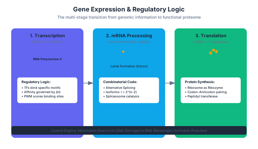
The transition of biology from a descriptive discipline to an information science is most evident in the study of Gene Expression and Regulation. At its core, this field examines the "Central Dogma"—the flow of biological information from DNA to RNA to Protein—while accounting for the sophisticated regulatory layers that allow a single genome to produce the diverse cellular phenotypes found in a multicellular organism.

The Logic of Transcription and Transcription Factors

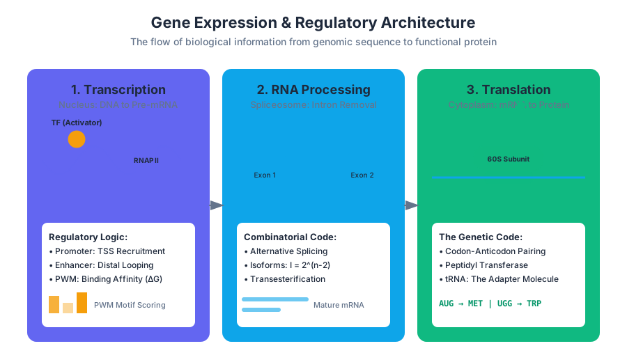
Transcription is the first stage of gene expression, where a specific segment of DNA is copied into RNA by the enzyme RNA Polymerase (RNAP). In eukaryotes, this process is not a simple "on/off" switch but a complex integration of signals processed by Transcription Factors (TFs).

The Thermodynamics of TF Binding

Transcription factors are proteins that bind to specific DNA sequences (motifs) to either recruit or block RNA Polymerase. The affinity of a TF for its binding site is governed by the Gibbs Free Energy ($\Delta G$) of the interaction. The probability $P$ of a site being occupied can be modeled using a Boltzmann distribution:

$$P_{bound} = \frac{1}{1 + e^{\frac{\Delta G - \mu}{kT}}}$$

where $\mu$ is the chemical potential of the TF in the nucleoplasm. This relationship implies that small changes in TF concentration or binding affinity (via mutation or modification) can lead to non-linear shifts in gene expression.

Enhancers and Promoters: The Regulatory Architecture

The regulatory landscape of a gene consists of:

1. Promoters: Located immediately upstream of the transcription start site (TSS).
2. Enhancers: Distal regulatory elements that can be thousands of base pairs away, brought into proximity with the promoter through DNA looping.

Element	Location	Function	Interaction Method
Core Promoter	-35 to +35 bp from TSS	Recruits General Transcription Factors (GTFs)	Direct binding of TATA-binding protein (TBP)
Proximal Promoter	Up to -250 bp	Fine-tunes transcription frequency	Binding of cell-specific TFs
Enhancer	Distal (Upstream/Downstream)	Amplifies transcription levels	DNA looping via Mediator complex
Silencer	Distal	Represses transcription	Recruitment of Histone Deacetylases (HDACs)

Implementation: Identifying Transcription Factor Binding Sites (TFBS)

In computational biology, we represent the binding preference of a TF using a Position Weight Matrix (PWM). The following Python snippet demonstrates how to score a DNA sequence against a known PWM to predict binding sites.

import numpy as np

def score_sequence(sequence, pwm):
    """
    Scores a DNA sequence against a Position Weight Matrix (PWM).
    sequence: str, e.g., "GCTAGTCAG"
    pwm: dict, mapping bases to numpy arrays of log-likelihoods
    """
    seq_len = len(sequence)
    pwm_len = len(pwm['A'])
    scores = []

    for i in range(seq_len - pwm_len + 1):
        sub_seq = sequence[i:i+pwm_len]
        score = 0
        for j, base in enumerate(sub_seq):
            if base in pwm:
                score += pwm[base][j]
            else:
                score -= 10 # Penalty for unknown bases
        scores.append(score)
    
    return scores

# Example PWM for a hypothetical TF (Log-odds ratios)
hypothetical_pwm = {
    'A': np.array([ 1.2, -0.5,  0.1,  2.0]),
    'C': np.array([-1.0,  1.5, -0.2, -1.5]),
    'G': np.array([-0.8, -1.2,  1.8, -0.5]),
    'T': np.array([ 0.5,  0.2, -1.7,  0.0])
}

dna_strand = "GCTAGTACTGATCGAT"
results = score_sequence(dna_strand, hypothetical_pwm)
print(f"Binding scores across sequence: {results}")

mRNA Splicing: The Combinatorial Code

In eukaryotes, the primary transcript (pre-mRNA) contains non-coding regions called introns and coding regions called exons. Splicing is the process of removing introns and ligating exons together to form a mature mRNA.

The Spliceosome Mechanics

The spliceosome, a massive ribonucleoprotein complex, catalyzes two successive transesterification reactions.

1. The 2'-OH of an adenine residue at the branch point attacks the 5' splice site.
2. The 3'-OH of the upstream exon attacks the 3' splice site, releasing the intron as a "lariat" structure.

Alternative Splicing: One Gene, Many Proteins

Alternative splicing allows a single gene to encode multiple protein isoforms, vastly increasing proteomic complexity without increasing genome size. This is a primary driver of evolutionary innovation in higher eukaryotes.

The Splicing Rule: The selection of splice sites is determined by a "splicing code" consisting of cis-acting elements (Exonic Splicing Enhancers/Silencers) and trans-acting factors (SR proteins and hnRNPs).

Mathematical Representation of Splicing Complexity

If a gene has $n$ exons that can be independently included or excluded, the theoretical number of isoforms $I$ is: $$I = 2^{(n-2)}$$ (Assuming the first and last exons are constitutive). For the Drosophila Dscam gene, which has 95 alternative exons, this results in over 38,000 potential protein isoforms—more than the total number of genes in the fly genome.

\text{Reaction 1: } \text{Exon1-G} + \text{A(branch)} \rightarrow \text{Exon1-OH} + \text{G-A(lariat)}
\text{Reaction 2: } \text{Exon1-OH} + \text{G-Exon2} \rightarrow \text{Exon1-Exon2} + \text{Lariat}

Ribosome Function and the Genetic Code

Translation is the process where the mature mRNA is decoded by the ribosome to synthesize a polypeptide chain. This represents the final stage of information transfer, converting a nucleotide sequence into a functional amino acid sequence.

The Ribosome as a Ribozyme

The ribosome is composed of two subunits (60S and 40S in eukaryotes). Crucially, the catalytic heart of the ribosome—the peptidyl transferase center—is composed of RNA, not protein. This supports the "RNA World" hypothesis, suggesting that life's fundamental machinery evolved from self-replicating RNA molecules.

Decoding the Genetic Code

The genetic code is:

1. Triplet: Three nucleotides (a codon) specify one amino acid.
2. Degenerate: Multiple codons can code for the same amino acid (e.g., leucine is coded by six different codons).
3. Non-overlapping: The reading frame is set by the start codon (AUG).

Feature	Description	Biological Significance
Wobble Base Pairing	Flexible pairing at the 3rd codon position	Allows one tRNA to recognize multiple codons
Kinetic Proofreading	Delay in GTP hydrolysis during tRNA selection	Increases translation fidelity to 1 error per $10^4$ amino acids
Ribosome Profiling	Sequencing of ribosome-protected fragments	Allows for "snapshots" of global translation activity

Example: Translation Initiation Pipeline

Translation initiation is the rate-limiting step of protein synthesis. In eukaryotes, this involves the recognition of the 5' cap and the scanning for the Kozak sequence.

# Bioinformatic pipeline to analyze translation efficiency from Ribo-seq data
# 1. Trim adapters from Ribo-seq reads
cutadapt -a AGATCGGAAGAGCACACGTCTGAACTCCAGTCA -o trimmed_ribo.fastq raw_ribo.fastq

# 2. Map reads to the transcriptome (excluding rRNA)
bowtie2 -x genome_index -U trimmed_ribo.fastq -S mapped_ribo.sam

# 3. Calculate Ribosome Protected Fragments (RPFs) per gene
samtools sort mapped_ribo.sam -o sorted_ribo.bam
bedtools multicov -bams sorted_ribo.bam -bed genes.bed > counts.txt

# 4. Normalize by mRNA abundance (RNA-seq) to get Translation Efficiency (TE)
# TE = RPF_abundance / mRNA_abundance

Epigenetics: The Software of the Genome

Epigenetics refers to heritable changes in gene expression that do not involve alterations to the underlying DNA sequence. If DNA is the "hardware," epigenetics is the "software" that determines which programs are run.

DNA Methylation

In vertebrates, DNA methylation occurs almost exclusively at CpG dinucleotides. The addition of a methyl group to the 5th carbon of cytosine (5mC) by DNA Methyltransferases (DNMTs) is generally associated with gene silencing.

Histone Modifications and Chromatin Remodeling

DNA is wrapped around histone octamers to form nucleosomes. The N-terminal tails of histones are subject to various post-translational modifications (PTMs):

• Acetylation (H3K9ac): Neutralizes the positive charge of histones, loosening the DNA-histone interaction and promoting transcription.
• Methylation (H3K27me3): Often associated with the formation of heterochromatin (tightly packed, inactive DNA).

Modification	Enzyme	Effect on Chromatin	Transcriptional State
Acetylation	HAT (Histone Acetyltransferase)	Open (Euchromatin)	Active
Deacetylation	HDAC (Histone Deacetylase)	Closed (Heterochromatin)	Repressed
Trimethylation (H3K4me3)	HMT (Histone Methyltransferase)	Open	Active (Promoter)
Trimethylation (H3K27me3)	PRC2 Complex	Closed	Silenced

The Epigenetic Landscape

Waddington’s "epigenetic landscape" describes how a pluripotent cell "rolls" down valleys of differentiation. As the cell matures, its epigenetic profile becomes increasingly locked, restricting its potential to change identity.

Systems Biology of Gene Regulation

Gene regulation is not a collection of isolated events but a networked system. Gene Regulatory Networks (GRNs) behave like electronic circuits, utilizing feedback loops to maintain homeostasis or drive developmental transitions.

Feedback Loops and Bistability

• Negative Feedback: A protein inhibits its own production, leading to oscillations or stable steady states (e.g., the circadian clock).
• Positive Feedback: A protein promotes its own production, creating a "bistable" switch where a cell can flip between two distinct states (e.g., cell fate determination).

Worked Example: The Lac Operon Logic

The lac operon in E. coli is the classic example of biological logic. It functions as an AND NOT gate:

• Condition A: Lactose is present (Inactivates the repressor).
• Condition B: Glucose is absent (Activates the CAP activator via cAMP).
• Result: Transcription occurs only if (Lactose) AND NOT (Glucose).

-- Conceptual representation of a Gene Expression Database
-- Querying for genes upregulated in Cancer vs Normal tissue with specific epigenetic marks

SELECT 
    g.gene_name, 
    e.expression_log_fold_change, 
    m.methylation_level
FROM 
    gene_expression_data e
JOIN 
    genes g ON e.gene_id = g.id
JOIN 
    epigenetic_marks m ON g.id = m.gene_id
WHERE 
    e.tissue_type = 'Adenocarcinoma'
    AND e.expression_log_fold_change > 2.0
    AND m.mark_type = 'H3K4me3'
ORDER BY 
    e.expression_log_fold_change DESC;

Common Pitfalls and Misconceptions

1. "DNA is Destiny": This ignores the massive influence of the environment on the epigenome. Identical twins have the same DNA but different epigenetic profiles as they age.
2. "One Gene = One Protein": Alternative splicing and post-translational modifications mean a single gene can produce hundreds of distinct functional entities.
3. "Junk DNA": Previously thought to be useless, non-coding DNA contains the majority of the genome's regulatory instructions (enhancers, silencers, and non-coding RNAs).
4. Transcription = Expression: A gene can be transcribed but never translated due to miRNA interference or riboswitch regulation.

Cell Structure and Organelle Dynamics

The eukaryotic cell is not merely a "bag of enzymes" but a highly partitioned chemical reactor. The transition from the relatively simple architecture of prokaryotes to the complex, compartmentalized nature of eukaryotes represents one of the most significant "phase transitions" in biological history. By isolating specific biochemical reactions within membrane-bound organelles, eukaryotes circumvent the diffusion limits that constrain bacterial size, allowing for a massive increase in genomic complexity and metabolic efficiency.

This section explores the mechanics of cellular compartmentalization, the evolutionary origins of these compartments via endosymbiosis, and the sophisticated logistics system—protein trafficking—that ensures the right molecular "cargo" reaches the correct "address."

The Evolutionary Genesis: Endosymbiotic Theory

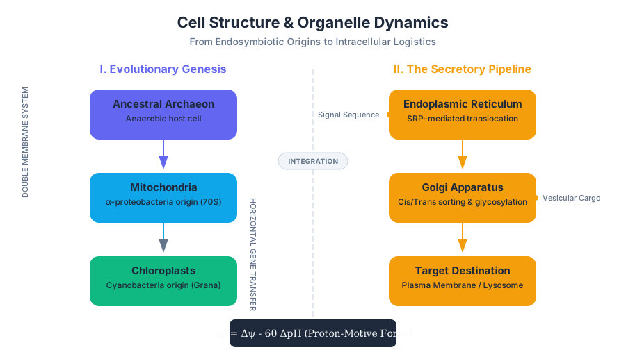
The Endosymbiotic Theory posits that the defining organelles of eukaryotic cells—mitochondria and chloroplasts—originated as independent prokaryotic organisms that were engulfed by a proto-eukaryotic host. Rather than being digested, these bacteria entered into a mutualistic relationship, eventually becoming obligate organelles.

The Mechanics of Integration

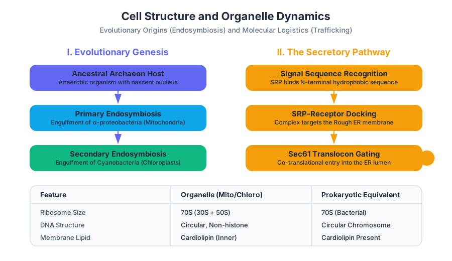
The theory, championed by Lynn Margulis in the 1960s, explains several "anomalies" in cell biology. Mitochondria are derived from α-proteobacteria, while chloroplasts are derived from cyanobacteria. The integration process involved a massive horizontal gene transfer (HGT), where the majority of the endosymbiont's genome was migrated to the host nucleus, leaving only a vestigial "mitogenome" or "plastid genome" behind.

Feature	Mitochondria / Chloroplasts	Prokaryotic Equivalent	Eukaryotic (Nuclear/Cytosolic)
DNA Structure	Circular, non-histone bound	Circular	Linear, histone-bound
Ribosome Size	70S (30S + 50S)	70S	80S (40S + 60S)
Division	Binary Fission	Binary Fission	Mitosis/Meiosis
Membrane	Double (Inner/Outer)	Single (plus peptidoglycan)	Single (Plasma membrane)
Initiator tRNA	fMet (formylmethionine)	fMet	Methionine

Evidence and Proofs

The strongest evidence for this theory lies in the double membrane system. The inner membrane of a mitochondrion contains cardiolipin, a phospholipid found almost exclusively in bacterial membranes and not in the eukaryotic plasma membrane. Furthermore, the sensitivity of mitochondrial ribosomes to antibiotics like streptomycin (which targets bacterial 70S ribosomes) but not to eukaryotic inhibitors provides a functional "smoking gun" for their bacterial ancestry.

The Serial Endosymbiosis Theory (SET): Evolution did not happen in a single step. First, an anaerobic archaeon likely engulfed an aerobic proteobacterium (forming the mitochondrion). Later, a subset of these now-aerobic eukaryotes engulfed a photosynthetic cyanobacterium, leading to the lineage of plants and algae.

Mitochondria and Chloroplasts: The Energy Transducers

Mitochondria and chloroplasts are the primary sites of energy conversion. While they share an endosymbiotic origin, their thermodynamic roles are inverse: mitochondria perform oxidative phosphorylation (catabolic), while chloroplasts perform photosynthesis (anabolic).

Mitochondrial Dynamics and the Chemiosmotic Gradient

The mitochondrion is structured to maximize the surface area of its inner membrane through folds called cristae. This is where the Electron Transport Chain (ETC) resides. The fundamental "algorithm" of the mitochondrion is the establishment of a proton-motive force ($\Delta p$).

The electrochemical potential gradient ($\Delta \mu_{H^+}$) is defined by the Nernst-Planck equation, but in biological systems, we simplify it to:

\Delta p = \Delta \psi - 60 \Delta pH

Where:

• $\Delta p$ is the proton-motive force (mV).
• $\Delta \psi$ is the electrical membrane potential.
• $\Delta pH$ is the pH gradient across the membrane.

Chloroplast Architecture

Chloroplasts contain a third membrane system: the thylakoids. These are stacked into grana, where the light-dependent reactions occur. The stroma (the fluid surrounding the thylakoids) contains the enzymes for the Calvin Cycle. Unlike mitochondria, which pump protons out of the matrix into the intermembrane space, chloroplasts pump protons from the stroma into the thylakoid lumen.

The Secretory Pathway and Protein Trafficking

If the cell is a factory, the Endoplasmic Reticulum (ER) and Golgi Apparatus constitute the assembly line and shipping department. Most proteins destined for the plasma membrane, secretion, or lysosomes must pass through this system.

The Signal Hypothesis

How does a protein "know" it belongs in the ER? This is governed by the Signal Hypothesis, for which Günter Blobel won the Nobel Prize. Proteins destined for the secretory pathway possess an N-terminal signal sequence (typically 16–30 hydrophobic amino acids).

1. Recognition: As the protein is translated, the Signal Recognition Particle (SRP) binds to the signal sequence.
2. Arrest: Translation pauses to prevent the protein from folding prematurely in the cytosol.
3. Targeting: The SRP-ribosome complex binds to the SRP receptor on the ER membrane.
4. Translocation: The ribosome is handed off to the Sec61 translocon, a protein-conducting channel. Translation resumes, and the protein is "threaded" into the ER lumen (co-translational translocation).

Low-Level Implementation: Translocon Gating Logic

In a systems-programming context, the translocon acts as a conditional gate. Below is a C-style representation of the logic gate governing protein entry into the ER.

/* 
 * Simulation of the Sec61 Translocon Gating Logic 
 * This represents the decision-making process for protein translocation.
 */

#include <stdio.h>
#include <stdbool.h>

typedef enum { CYTOSOL, ER_LUMEN, MEMBRANE } Destination;

struct Protein {
    char* sequence;
    bool has_signal_peptide;
    int hydrophobicity_index;
};

Destination route_protein(struct Protein* p) {
    // Check for Signal Recognition Particle (SRP) binding
    if (!p->has_signal_peptide) {
        return CYTOSOL; // Default destination
    }

    // Translocon (Sec61) interaction
    printf("SRP bound. Targeting to ER Translocon...\n");

    // Check for Stop-Transfer Anchor Sequence (STAS)
    // If a highly hydrophobic segment is found, it embeds in the membrane
    if (p->hydrophobicity_index > 80) {
        return MEMBRANE; 
    }

    return ER_LUMEN;
}

int main() {
    struct Protein insulin = {"MALWMRLLPLLALLALWGPDPAAA...", true, 45};
    Destination dest = route_protein(&insulin);
    printf("Protein routed to: %s\n", (dest == ER_LUMEN) ? "ER Lumen" : "Other");
    return 0;
}

The Endoplasmic Reticulum (ER): Quality Control

The ER is divided into the Rough ER (studded with ribosomes) and the Smooth ER (site of lipid synthesis and detoxification).

Protein Folding and N-linked Glycosylation

Once inside the ER lumen, proteins undergo critical modifications. The most important is N-linked glycosylation, where a pre-assembled 14-sugar oligosaccharide is transferred to an Asparagine (Asn) residue within the motif Asn-X-Ser/Thr.

This sugar tag acts as a "quality control" marker. Chaperone proteins like Calnexin and Calreticulin bind to these sugars to ensure the protein folds correctly. If a protein fails to fold after multiple attempts, it is ejected back into the cytosol for degradation via the ER-Associated Degradation (ERAD) pathway.

Signal Sequence Motif	Destination	Recognition Factor
N-terminal Hydrophobic	ER Lumen / Membrane	SRP (Signal Recognition Particle)
KDEL (C-terminal)	ER Retention	KDEL Receptor (Golgi-to-ER)
SKL (C-terminal)	Peroxisome	Pex5
Arg/Lys Rich (NLS)	Nucleus	Importin α/β
Mannose-6-Phosphate	Lysosome	M6P Receptor

The Golgi Apparatus: The Sorting Hub

The Golgi is a series of flattened stacks called cisternae. It is polarized, with a cis face (receiving) and a trans face (shipping).

The Cisternal Maturation Model

There are two competing theories on how cargo moves through the Golgi. The current consensus is the Cisternal Maturation Model, which suggests that the cisternae themselves "age" and move from cis to trans, changing their enzymatic composition over time, while the processing enzymes are recycled backward via COPI vesicles.

Post-Translational Modification

In the Golgi, the N-linked oligosaccharides added in the ER are trimmed and modified. Some proteins receive O-linked glycosylation (sugars added to Oxygen on Ser/Thr). The Golgi also performs "proteolytic processing"—for example, converting proinsulin into active insulin by snipping out the C-peptide.

Vesicular Transport: The Logistics of "Bud and Fuse"

Movement between the ER, Golgi, and plasma membrane is mediated by small, membrane-bound vesicles. This process requires two distinct steps: budding (forming the vesicle) and fusion (merging with the target).

Vesicle Coats

Vesicles do not form spontaneously; they are sculpted by "coat proteins" that deform the membrane into a sphere and select the cargo.

Coat Type	Direction	Major Components
COPII	ER $\rightarrow$ cis-Golgi (Anterograde)	Sar1 GTPase, Sec23/24, Sec13/31
COPI	Golgi $\rightarrow$ ER (Retrograde)	Arf GTPase, Coatomer
Clathrin	Golgi $\rightarrow$ Lysosome / Plasma Membrane	Clathrin, AP-1/AP-2 adaptors

The SNARE Hypothesis: Ensuring Specificity

How does a vesicle from the Golgi know to fuse with the plasma membrane and not a mitochondrion? This is controlled by SNARE proteins.

• v-SNAREs (vesicle) bind to specific t-SNAREs (target).
• The interaction forms a highly stable four-helix bundle that "zips" the two membranes together, overcoming the electrostatic repulsion between phospholipid headgroups.

Mathematical Derivation: The Energy of Membrane Fusion

The energy required to bring two membranes close enough to fuse (the "hydration barrier") is significant. The SNARE complex must release enough free energy ($\Delta G$) to overcome this.

\Delta G_{fusion} \approx \gamma \cdot \Delta A + W_{hydration}

Where:

• $\gamma$ is the surface tension of the membrane.
• $\Delta A$ is the change in surface area.
• $W_{hydration}$ is the work required to remove water molecules between bilayers.

SNARE zipping provides approximately 35 $k_BT$ of energy, which is sufficient to drive the formation of a fusion pore.

Real-World Application: Analyzing Signal Peptides

In bioinformatics, identifying these trafficking signals is crucial for predicting protein function. We can use Python to analyze the hydrophobicity of a sequence to predict if it contains an ER signal peptide.

import matplotlib.pyplot as plt

def kyte_doolittle_hydrophobicity(sequence, window_size=11):
    """
    Calculates the hydrophobicity profile of a protein sequence.
    High values indicate hydrophobic regions (potential signal peptides or TM domains).
    """
    kd_scale = {
        'A': 1.8, 'R': -4.5, 'N': -3.5, 'D': -3.5, 'C': 2.5,
        'Q': -3.5, 'E': -3.5, 'G': -0.4, 'H': -3.2, 'I': 4.5,
        'L': 3.8, 'K': -3.9, 'M': 1.9, 'F': 2.8, 'P': -1.6,
        'S': -0.8, 'T': -0.7, 'W': -0.9, 'Y': -1.3, 'V': 4.2
    }
    
    scores = []
    for i in range(len(sequence) - window_size + 1):
        window = sequence[i:i + window_size]
        score = sum(kd_scale.get(aa, 0) for aa in window) / window_size
        scores.append(score)
    return scores

# Example: Human Insulin Signal Peptide (First 24 residues)
insulin_seq = "MALWMRLLPLLALLALWGPDPAAA"
profile = kyte_doolittle_hydrophobicity(insulin_seq)

print(f"Max Hydrophobicity: {max(profile):.2f}")
# A score > 1.6 in the first 30 residues is a strong indicator of an ER signal.

Lysosomes and Peroxisomes: The Waste Management System

While the ER and Golgi are for synthesis, the lysosomes and peroxisomes are for degradation.

Lysosomes: The Acidic Stomach

Lysosomes contain acid hydrolases—enzymes that break down polymers (proteins, lipids, nucleic acids). These enzymes only function at a pH of ~5.0. This is a "fail-safe" mechanism: if a lysosome ruptures, the enzymes will denature in the neutral pH (~7.2) of the cytosol, preventing the cell from digesting itself.

Peroxisomes: Oxidative Detox

Peroxisomes handle long-chain fatty acid oxidation and the detoxification of compounds like alcohol. They produce hydrogen peroxide ($H_2O_2$) as a byproduct, which is immediately neutralized by the enzyme catalase.

Clinical Correlation: Zellweger Syndrome is a genetic disorder where peroxisomes fail to assemble correctly. This leads to the accumulation of very-long-chain fatty acids, causing severe neurological damage, as the brain relies heavily on peroxisomal lipid processing for myelin formation.

Summary of Organelle Dynamics

The eukaryotic cell functions as a distributed system. The "state" of the cell is maintained by constant flux—vesicles budding from one compartment and fusing with another.

Organelle	Primary Metabolic / Structural Role	Industrial Analogue
Nucleus	Genomic storage, RNA synthesis	Headquarters / Blueprint Archive
ER (Rough)	Protein synthesis and folding	Factory Floor (Assembly)
ER (Smooth)	Lipid synthesis, $Ca^{2+}$ storage	Chemical Processing Plant
Golgi	Protein modification and sorting	Distribution Center / Mailroom
Mitochondria	ATP production (Aerobic)	Power Plant
Lysosome	Macromolecule degradation	Recycling Center
Peroxisome	Redox signaling, Lipid oxidation	Hazardous Waste Treatment

Edge Case: Retrograde Transport and Toxins

Some pathogens hijack the secretory pathway in reverse. Ricin (from castor beans) and Shiga toxin enter the cell via endocytosis, travel backward through the Golgi to the ER, and then "escape" into the cytosol by mimicking unfolded proteins. They then deactivate ribosomes, halting all protein synthesis and killing the cell.

# Conceptual "Configuration" of a Secretory Protein
protein_metadata:
  name: "Insulin"
  translation_site: "Rough ER"
  pathway:
    - step: 1
      action: "Co-translational translocation"
      signal: "N-terminal hydrophobic alpha-helix"
    - step: 2
      action: "N-linked Glycosylation"
      site: "Asn-X-Ser/Thr"
    - step: 3
      action: "COPII Budding"
      destination: "Cis-Golgi"
    - step: 4
      action: "Proteolytic Cleavage"
      result: "Removal of C-peptide"
    - step: 5
      action: "Clathrin-mediated sorting"
      destination: "Secretory Granule"

Mendelian Genetics and Meiosis

The transition from molecular biochemistry—the study of lipids, proteins, and nucleic acids—to organismal biology is bridged by the mechanics of inheritance. While DNA provides the blueprint, the cellular machinery of meiosis and the statistical laws of Mendelian genetics dictate how that blueprint is partitioned, shuffled, and transmitted across generations. This section explores the rigorous logic of heredity, treating the genome not as a static library, but as a dynamic system of discrete units (alleles) governed by the laws of probability and chromosomal movement.

The Cellular Engine: Meiosis

Meiosis is a specialized form of cell division that reduces the chromosome number by half, resulting in the production of haploid gametes (sperm and eggs). Unlike mitosis, which aims for clonal fidelity, meiosis is designed for genetic variation. It consists of one round of DNA replication followed by two successive rounds of nuclear division: Meiosis I and Meiosis II.

Meiosis I: The Reductional Division

In Meiosis I, homologous chromosomes—pairs of chromosomes containing the same genes but potentially different alleles—pair up and then separate. This stage is "reductional" because it reduces the ploidy from diploid ($2n$) to haploid ($n$).

1. Prophase I: This is the most complex phase. Homologous chromosomes undergo synapsis, forming a tetrad (or bivalent). During this time, crossing over (recombination) occurs at sites called chiasmata. This is the physical exchange of genetic material between non-sister chromatids.
2. Metaphase I: Homologous pairs align at the metaphase plate. Crucially, the orientation of each pair is random—a phenomenon that forms the physical basis for Mendel’s Law of Independent Assortment.
3. Anaphase I: Homologous chromosomes are pulled to opposite poles. Note that sister chromatids remain attached at their centromeres.
4. Telophase I and Cytokinesis: Two haploid daughter cells form, each containing one chromosome from every homologous pair.

Meiosis II: The Equational Division

Meiosis II resembles mitosis. The sister chromatids, which are no longer identical due to crossing over in Prophase I, are finally separated.

1. Prophase II: Spindle apparatus reforms.
2. Metaphase II: Chromosomes align at the equator.
3. Anaphase II: Centromeres dissolve, and sister chromatids move to opposite poles.
4. Telophase II: Nuclear envelopes reform, resulting in four genetically distinct haploid cells.

Feature	Mitosis	Meiosis I	Meiosis II
Purpose	Somatic growth / Repair	Diversity / Ploidy reduction	Gamete maturation
Homologous Pairing	No	Yes (Synapsis)	No
Crossing Over	No	Yes (Prophase I)	No
Outcome	2 Identical Diploid ($2n$)	2 Unique Haploid ($n$)	4 Unique Haploid ($n$)
Chromatid Separation	Anaphase	Anaphase II	Anaphase II

Mendelian Laws of Inheritance

Gregor Mendel’s work in the mid-19th century transformed biology into a predictive science. By studying discrete traits in Pisum sativum, he deduced that inheritance is "particulate"—driven by discrete units we now call genes.

The Law of Segregation

Theorem: During gamete formation, the two alleles for a heritable character segregate (separate) from each other and end up in different gametes.

This law corresponds to the separation of homologous chromosomes during Anaphase I. If an organism has the genotype $Aa$, 50% of its gametes will receive the $A$ allele and 50% will receive the $a$ allele.

The Law of Independent Assortment

Theorem: Each pair of alleles segregates independently of each other pair of alleles during gamete formation.

This law applies only to genes located on different chromosomes (or very far apart on the same chromosome). It is the direct result of the random orientation of homologous pairs during Metaphase I.

Mathematical Framework of Mendelian Crosses

To predict outcomes, we use the Product Rule (for independent events: $P(A \text{ and } B) = P(A) \times P(B)$) and the Sum Rule (for mutually exclusive events: $P(A \text{ or } B) = P(A) + P(B)$).

# Low-level implementation of a Mendelian Cross Simulator
# This script calculates genotype frequencies for a dihybrid cross (AaBb x AaBb)

from collections import Counter
from itertools import product

def simulate_cross(parent1_genotype, parent2_genotype):
    """
    Simulates a genetic cross between two parents.
    Genotypes are represented as strings, e.g., 'Aa', 'Bb'.
    """
    # Split genotypes into individual alleles
    p1_alleles = [parent1_genotype[i:i+2] for i in range(0, len(parent1_genotype), 2)]
    p2_alleles = [parent2_genotype[i:i+2] for i in range(0, len(parent2_genotype), 2)]
    
    # Generate possible gametes for each parent
    def get_gametes(genotype_list):
        return ["".join(g) for g in product(*[list(gene) for gene in genotype_list])]

    gametes1 = get_gametes(p1_alleles)
    gametes2 = get_gametes(p2_alleles)
    
    # Create offspring by combining gametes
    offspring_genotypes = []
    for g1 in gametes1:
        for g2 in gametes2:
            # Sort alleles within each gene to keep 'Aa' and 'aA' consistent
            combined = ""
            for i in range(len(g1)):
                gene_pair = sorted([g1[i], g2[i]])
                combined += "".join(gene_pair)
            offspring_genotypes.append(combined)
            
    counts = Counter(offspring_genotypes)
    total = len(offspring_genotypes)
    
    return {genotype: f"{count}/{total}" for genotype, count in counts.items()}

# Example: Dihybrid Cross AaBb x AaBb
results = simulate_cross("AaBb", "AaBb")
for genotype, ratio in sorted(results.items()):
    print(f"Genotype: {genotype} | Probability: {ratio}")

Chromosomal Errors: Nondisjunction

The fidelity of meiosis is paramount. When the machinery fails to separate chromosomes or chromatids correctly, the result is nondisjunction. This leads to aneuploidy, a condition where cells have an abnormal number of chromosomes.

Mechanisms of Nondisjunction

1. Meiosis I Nondisjunction: Homologous chromosomes fail to separate. Result: All four gametes are abnormal ($n+1, n+1, n-1, n-1$).
2. Meiosis II Nondisjunction: Sister chromatids fail to separate. Result: Two normal gametes, two abnormal ($n+1, n-1, n, n$).

Condition	Genotype	Clinical Manifestation
Down Syndrome	Trisomy 21	Cognitive impairment, distinct facial features, heart defects.
Klinefelter Syndrome	XXY	Male phenotype, sterile, some female secondary characteristics.
Turner Syndrome	X0	Female phenotype, sterile, short stature (only viable monosomy).
Patau Syndrome	Trisomy 13	Severe neurological and circulatory defects; short life expectancy.

Pedigree Analysis: The Logic of Inheritance

In human genetics, we cannot perform controlled crosses. Instead, we use pedigrees—diagrams showing the phenotypes of family members across generations—to deduce genotypes and inheritance patterns.

Key Patterns to Recognize

• Autosomal Dominant: The trait appears in every generation. Every affected person has at least one affected parent.
• Autosomal Recessive: The trait can skip generations. Affected individuals are often born to unaffected (carrier) parents.
• X-Linked Recessive: More common in males. Affected fathers pass the allele to all daughters (who become carriers) but no sons.
• X-Linked Dominant: Affected fathers pass the trait to all daughters and no sons.

\begin{aligned}
&\text{Probability Logic for Pedigrees:} \\
&\text{If } P(\text{Carrier Parent 1}) = p \text{ and } P(\text{Carrier Parent 2}) = q, \\
&\text{Then } P(\text{Affected Child}) = p \times q \times \frac{1}{4} \text{ (for Autosomal Recessive)} \\
\\
&\text{Bayes' Theorem Application:} \\
&P(\text{Carrier} | \text{Unaffected}) = \frac{P(\text{Unaffected} | \text{Carrier})P(\text{Carrier})}{P(\text{Unaffected})}
\end{aligned}

Worked Example: Pedigree Logic

Suppose a couple is unaffected, but the man's brother has an autosomal recessive disease (genotype $aa$). What is the probability their first child will be affected?

1. The man's parents must be carriers ($Aa \times Aa$).
2. The man is unaffected, so his possible genotypes are $AA$ or $Aa$. The probability he is a carrier ($Aa$) is $2/3$ (since we exclude $aa$).
3. We must know the carrier frequency of the woman. If she is from the general population where the carrier frequency is $1/50$:
4. $P(\text{Affected child}) = P(\text{Father is } Aa) \times P(\text{Mother is } Aa) \times P(\text{Child is } aa | \text{Parents } Aa)$
5. $P = (2/3) \times (1/50) \times (1/4) = 2/600 = 1/300$.

Real-World Application: Variant Calling

In modern bioinformatics, Mendelian laws are used to filter "noise" in DNA sequencing data. When sequencing a "trio" (mother, father, and child), any variant in the child that does not follow Mendelian inheritance (e.g., child is $AA$ while both parents are $aa$) is flagged as a potential sequencing error or a de novo mutation.

# Using bcftools to filter for Mendelian violations in a VCF (Variant Call Format) file
# This is a common step in clinical diagnostics for rare diseases.

# 1. Define the trio relationship in a PED file (FamilyID, SampleID, FatherID, MotherID, Sex, Phenotype)
echo "FAM01 CHILD01 FATHER01 MOTHER01 1 2" > trio.ped

# 2. Use bcftools to find Mendelian violations
# +mendelian plugin checks for inconsistencies
bcftools +mendelian input_variants.vcf.gz -p trio.ped -m list > violations.txt

# 3. Output format:
# [1] Chromosome [2] Position [3] Violation Type (e.g., "GT: child is 0/0, parents are 1/1")

Common Pitfalls and Edge Cases

1. Linked Genes: Mendel’s Second Law (Independent Assortment) fails if genes are close together on the same chromosome. They will be inherited together unless a crossover event occurs between them.
2. Incomplete Dominance vs. Codominance: In incomplete dominance, the heterozygote has an intermediate phenotype (e.g., pink flowers from red and white parents). In codominance, both alleles are expressed fully (e.g., AB blood type).
3. Lethal Alleles: Some genotypes (usually homozygous dominant or recessive) result in prenatal death, which skews the observed Mendelian ratios (e.g., a 2:1 ratio instead of 3:1).
4. Nondisjunction Timing: Students often confuse the results of Meiosis I vs. Meiosis II nondisjunction. Remember: Meiosis I failure results in gametes with both homologs; Meiosis II failure results in gametes with two copies of the same sister chromatid.

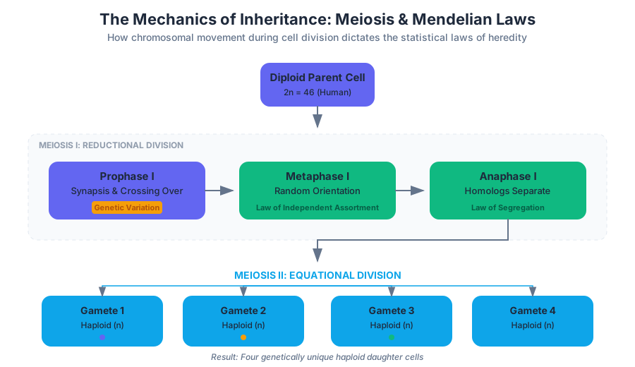
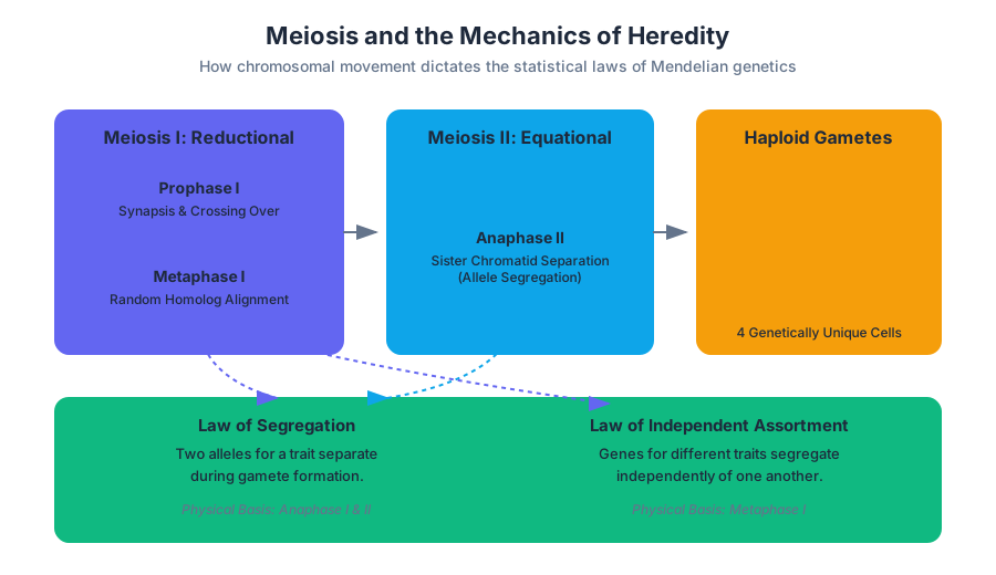
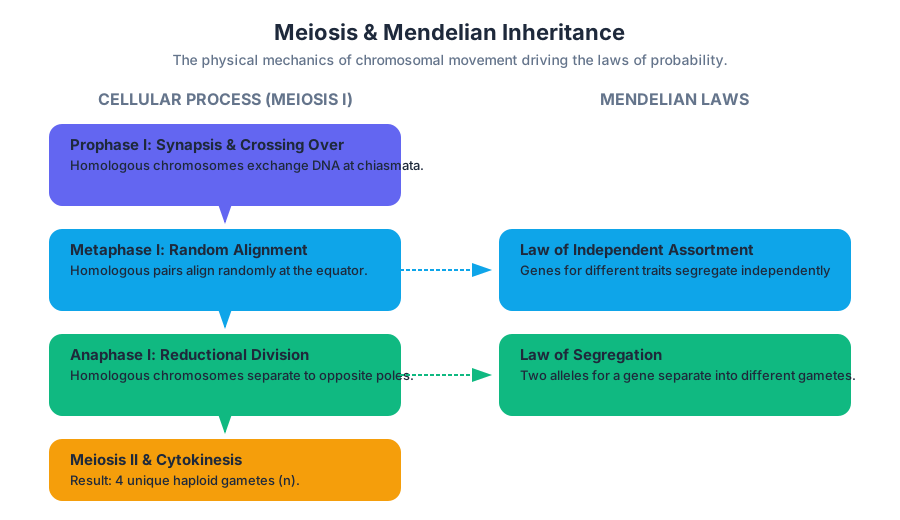
Genetic Mapping and Linkage

The fundamental law of Mendelian genetics is the Law of Independent Assortment, which posits that alleles of different genes segregate independently during gamete formation. However, as the field of genetics matured in the early 20th century, researchers like Thomas Hunt Morgan and Alfred Sturtevant discovered that certain genes are "linked"—they travel together on the same chromosome.

Genetic Mapping is the process of determining the relative positions of genes on a chromosome based on how often they are separated by recombination. This section explores the transition from qualitative inheritance to quantitative spatial mapping, providing the mathematical and experimental framework for understanding the architecture of the genome.

The Physical Basis of Linkage

Linkage occurs when two loci are located on the same physical DNA molecule (chromosome). During Prophase I of meiosis, homologous chromosomes undergo synapsis, forming a synaptonemal complex where genetic material is exchanged. This process, known as crossing over or recombination, is the only mechanism by which alleles on the same chromosome can be uncoupled.

The Linkage Principle: The probability of a crossover occurring between two loci is proportional to the physical distance between them. The further apart two genes are, the more likely a recombination event will occur in the intervening space.

Recombination Frequency (RF)

The Recombination Frequency is the primary metric used to estimate genetic distance. It is calculated as the ratio of recombinant offspring to the total number of offspring.

$$RF = \frac{\text{Number of Recombinant Progeny}}{\text{Total Number of Progeny}} \times 100$$

By convention, an $RF$ of 1% is defined as one Centimorgan (cM), also known as a map unit (m.u.).

Recombination and Map Distance

While $RF$ is a reliable proxy for distance at short intervals, it is not perfectly linear over long distances. This is because multiple crossovers can occur between two distant genes. A double crossover between two genes restores the original parental allele combination, making the offspring appear as "non-recombinants" even though recombination occurred.

The 50% Limit

Even if two genes are at opposite ends of a very long chromosome, the maximum observed $RF$ is 50%. This is because recombination involves only two of the four chromatids in a meiotic bivalent. At great distances, the genes assort as if they were on different chromosomes (independent assortment).

Parameter	Definition	Typical Range
Linkage	Genes on the same chromosome	0 - 50 cM
Synteny	Genes physically on the same chromosome	Any distance
Map Unit (cM)	1% Recombination Frequency	0.1 - 50 cM
Physical Distance	Base pairs (bp)	Varies by species (e.g., ~1Mb/cM in humans)

Calculating Recombination in a Two-Point Cross

To calculate the distance between two genes, $A$ and $B$, we perform a testcross. We cross a double heterozygote ($AaBb$) with a double homozygous recessive ($aabb$).

# Low-level implementation: Calculating Recombination Frequency from Cross Data
def calculate_map_distance(counts):
    """
    Calculates the recombination frequency (RF) and map distance.
    'counts' is a dict: {'parental': int, 'recombinant': int}
    """
    total = sum(counts.values())
    if total == 0:
        raise ValueError("Total progeny cannot be zero.")
    
    rf = (counts['recombinant'] / total) * 100
    
    # Apply a simple correction if RF approaches 50% (Haldane Mapping Function)
    import math
    if rf < 50:
        # Haldane's mapping function: d = -1/2 * ln(1 - 2*RF)
        # RF is expressed as a fraction here
        rf_fraction = rf / 100
        haldane_distance = -0.5 * math.log(1 - 2 * rf_fraction) * 100
    else:
        haldane_distance = float('inf')
        
    return {
        "Observed_RF": round(rf, 2),
        "Haldane_cM": round(haldane_distance, 2)
    }

# Example Data: 400 Parental, 100 Recombinant
data = {'parental': 400, 'recombinant': 100}
result = calculate_map_distance(data)
print(f"Map Distance: {result['Observed_RF']} cM")

The Three-Point Cross

The Three-Point Cross is the definitive method for determining the order and distance of three linked genes ($A, B, C$) in a single experiment. It is superior to two-point crosses because it allows for the detection of double crossovers (DCOs), which are the rarest classes of offspring.

Step-by-Step Logic

1. Identify Parental Classes: The two most frequent phenotypic classes are the parentals (no crossovers).
2. Identify Double Crossover (DCO) Classes: The two least frequent classes result from two recombination events.
3. Determine Gene Order: Compare the parentals to the DCOs. The gene that "swaps" relative to the other two in the DCO classes is the gene in the middle.
4. Calculate SCO Distances: Sum the Single Crossovers (SCO) and DCOs for each interval and divide by the total.

Interference and Coincidence

In most organisms, a crossover in one region of the chromosome reduces the probability of a second crossover nearby. This phenomenon is called chromosomal interference.

Coefficient of Coincidence ($C$): The ratio of observed DCOs to expected DCOs. $$C = \frac{\text{Observed DCO Frequency}}{\text{Expected DCO Frequency}}$$ Interference ($I$): $I = 1 - C$. If $I = 1$, interference is complete (no DCOs). If $I = 0$, crossovers are independent.

% Mathematical derivation of Expected DCOs
\text{Expected DCO} = RF(\text{Interval 1}) \times RF(\text{Interval 2}) \times \text{Total Progeny}

% Example:
% Interval A-B = 0.10 (10 cM)
% Interval B-C = 0.20 (20 cM)
% Total Progeny = 1000
\text{Expected DCO} = 0.10 \times 0.20 \times 1000 = 20

Offspring Phenotype	Count	Class
$v\ cv\ ct$	580	Parental
$+\ +\ +$	592	Parental
$v\ +\ +$	45	SCO (v-cv)
$+\ cv\ ct$	40	SCO (v-cv)
$v\ cv\ +$	89	SCO (cv-ct)
$+\ +\ ct$	94	SCO (cv-ct)
$v\ +\ ct$	3	DCO
$+\ cv\ +$	5	DCO

Yeast Tetrad Analysis

In fungi like Saccharomyces cerevisiae, the four products of a single meiosis are held together in a sac called an ascus. Analyzing these tetrads allows geneticists to look directly at the results of recombination without the statistical noise of random fertilization.

Tetrad Types

When crossing two strains ($AB \times ab$), three types of tetrads can be produced:

1. Parental Ditype (PD): Contains four parental spores ($2 AB, 2 ab$).
2. Non-Parental Ditype (NPD): Contains four recombinant spores ($2 Ab, 2 aB$). This occurs via a four-strand double crossover.
3. Tetratype (TT): Contains two parental and two recombinant spores ($1 AB, 1 ab, 1 Ab, 1 aB$). This occurs via a single crossover.

Mapping Formula for Tetrads

Linkage is identified when $PD \gg NPD$. The distance is calculated using the formula:

$$cM = \frac{1/2 TT + 3 NPD}{\text{Total Tetrads}} \times 100$$

The $3 \times NPD$ term is a correction factor that accounts for multiple crossovers that result in NPDs.

Relationship	Ratio	Conclusion
Independent Assortment	$PD \approx NPD$	Genes on different chromosomes
Linkage	$PD \gg NPD$	Genes on the same chromosome
Centromere Linkage	Low $TT$ frequency	Genes close to their respective centromeres

SNP Mapping and Modern Genomics

In modern human genetics, we rarely use phenotypic markers like "curly hair" or "eye color" for mapping. Instead, we use Single Nucleotide Polymorphisms (SNPs)—single-base variations in the DNA sequence.

LOD Scores

Because human families are small, we cannot use simple recombination frequencies to map disease genes. Instead, we use the LOD Score (Logarithm of the Odds).

LOD Score Definition: The log-ratio of the likelihood that two loci are linked at a specific distance ($\theta$) versus the likelihood that they are unlinked ($\theta = 0.5$). $$LOD = \log_{10} \left( \frac{\text{Likelihood of linkage at } \theta}{\text{Likelihood of independent assortment}} \right)$$

• LOD > 3.0: Statistically significant evidence for linkage (1000:1 odds).
• LOD < -2.0: Evidence against linkage.

Genome-Wide Association Studies (GWAS)

GWAS leverages Linkage Disequilibrium (LD)—the non-random association of alleles at different loci. If a specific SNP is consistently found in patients with a disease, that SNP is likely "linked" to the causal mutation.

# Example: Using PLINK (a standard tool) to perform linkage analysis
# This command calculates the LD (r-squared) between SNPs in a window
plink --bfile human_data \
      --ld-window-kb 500 \
      --ld-window-r2 0.2 \
      --out study_results \
      --make-founders

Mapping Functions: Haldane vs. Kosambi

As mentioned, $RF$ is not additive over long distances. Mapping functions translate observed $RF$ into more accurate map distances (cM) by modeling the probability of multiple crossovers.

1. Haldane Mapping Function: Assumes no interference. Crossovers occur randomly according to a Poisson distribution. $$d = -\frac{1}{2} \ln(1 - 2 \cdot RF)$$
2. Kosambi Mapping Function: Accounts for interference, assuming that one crossover inhibits another nearby. This is generally more accurate for most eukaryotic chromosomes. $$d = \frac{1}{4} \ln \left( \frac{1 + 2 \cdot RF}{1 - 2 \cdot RF} \right)$$

Common Pitfalls in Mapping

• Underestimating Distance: Failing to account for double crossovers leads to "shorter" maps. This is why three-point crosses are preferred over two-point crosses.
• Sex-Specific Differences: In many species, recombination rates differ between sexes. In Drosophila, recombination occurs only in females. In humans, females generally have higher recombination rates than males.
• Hotspots and Coldspots: Recombination is not uniform across the chromosome. Centromeres are typically recombination "coldspots," while other regions are "hotspots." Consequently, genetic distance (cM) does not always map linearly to physical distance (bp).

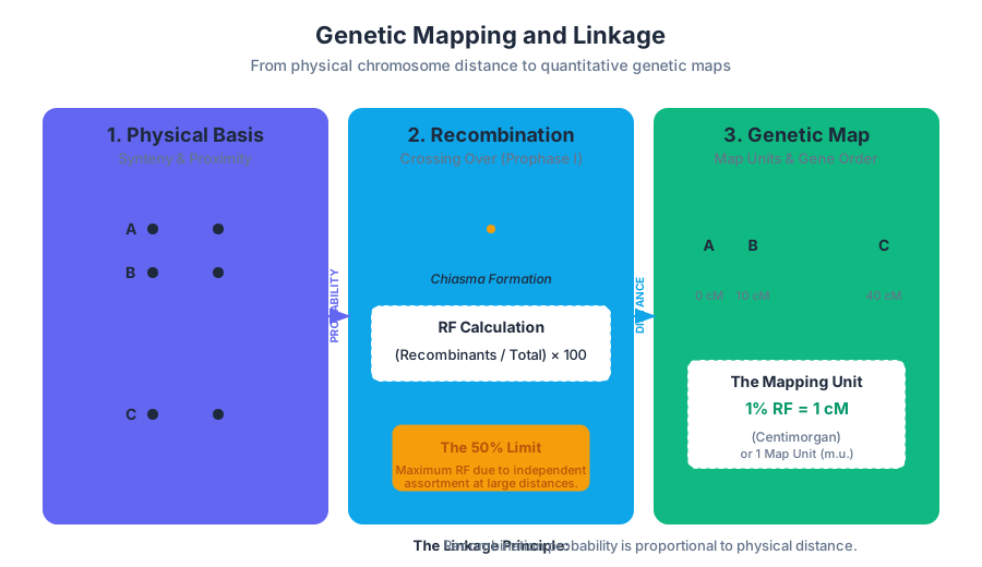
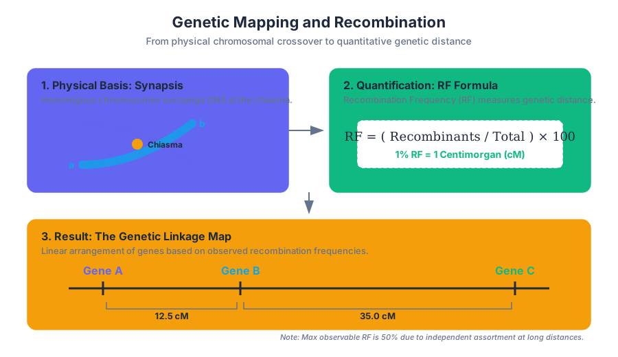
Recombinant DNA Technology

Recombinant DNA (rDNA) technology represents the pinnacle of the "Molecular Biology Revolution," transitioning biology from a purely descriptive science to a manipulative, engineering-oriented discipline. At its core, rDNA technology involves the joining together of DNA molecules from different species and the subsequent insertion of this hybrid DNA into a host organism to produce new genetic combinations. This "cut-and-paste" capability allows scientists to isolate specific genes, amplify them, and express their encoded proteins in heterologous systems, such as producing human insulin in Escherichia coli.

The Molecular Toolkit: Restriction Endonucleases

Before we can manipulate DNA, we must be able to cut it at precise, predictable locations. In nature, Restriction Endonucleases (or restriction enzymes) serve as a primitive immune system for bacteria, "restricting" the entry of foreign viral DNA by cleaving it.

What it is

Restriction enzymes are proteins that recognize specific, usually palindromic, DNA sequences (4–8 base pairs in length) and catalyze the hydrolysis of the phosphodiester backbone.

Definition: Palindromic Symmetry In the context of double-stranded DNA, a palindrome occurs when the sequence of the "top" strand (5' to 3') is identical to the "bottom" strand (5' to 3'). For example: 5'-GAATTC-3' 3'-CTTAAG-5'

How it works: Sticky vs. Blunt Ends

Enzymes like EcoRI make staggered cuts, leaving short, single-stranded overhangs known as sticky ends. These ends are highly useful because they can spontaneously re-anneal via hydrogen bonding with any other DNA fragment cut by the same enzyme. Conversely, enzymes like SmaI cut straight across the helix, producing blunt ends, which are harder to ligate but more versatile as they do not require sequence complementarity.

Enzyme	Source Organism	Recognition Sequence (5'→3')	Cut Type
EcoRI	Escherichia coli	G^AATTC	Sticky (5' overhang)
HindIII	Haemophilus influenzae	A^AGCTT	Sticky (5' overhang)
PstI	Providencia stuartii	CTGCA^G	Sticky (3' overhang)
SmaI	Serratia marcescens	CCC^GGG	Blunt
NotI	Nocardia otitidis	GC^GGCCGC	Sticky (Rare cutter)

Implementation: Simulating a Digest

In a computational context, we often need to predict the fragments generated by a digest to verify our experimental design.

import re

def simulate_digest(sequence, recognition_site, cut_offset):
    """
    Simulates a restriction digest on a linear DNA sequence.
    :param sequence: The DNA string (5' to 3')
    :param recognition_site: The string to search for (e.g., 'GAATTC')
    :param cut_offset: Index within the site where the cut occurs
    :return: List of DNA fragments
    """
    # Find all occurrences of the recognition site
    sites = [m.start() for m in re.finditer(recognition_site, sequence)]
    
    fragments = []
    last_cut = 0
    
    for site_start in sites:
        cut_index = site_start + cut_offset
        fragments.append(sequence[last_cut:cut_index])
        last_cut = cut_index
        
    fragments.append(sequence[last_cut:])
    return fragments

# Example: Digesting a sequence with EcoRI (G^AATTC)
dna_seq = "ATGCGAGAATTCGCTAGCTGAATTCGATCGA"
ecoRI_site = "GAATTC"
result = simulate_digest(dna_seq, ecoRI_site, 1)

print(f"Fragments: {result}")
# Output: ['ATGCGAG', 'AATTCGCTAGCTG', 'AATTCGATCGA']

Plasmid Vectors: The Vehicles of Cloning

Once a gene of interest is isolated, it must be placed into a Vector—a DNA molecule capable of autonomous replication within a host cell. The most common vectors are Plasmids, small, circular, extrachromosomal DNA molecules found in bacteria.

Anatomy of a Cloning Vector

A functional cloning vector must possess three essential features:

1. Origin of Replication (ori): A specific DNA sequence where replication begins. This determines the "copy number" (how many plasmids exist per cell).
2. Selectable Marker: Usually an antibiotic resistance gene (e.g., $Amp^R$). This allows researchers to kill off any bacteria that did not successfully take up the plasmid.
3. Multiple Cloning Site (MCS): A short region containing several unique restriction sites, providing a "docking port" for the insertion of foreign DNA.

The Ligation Reaction

The process of joining the vector and the insert is called Ligation, catalyzed by the enzyme DNA Ligase. Ligase uses ATP to repair the phosphate backbone between the 3'-OH of one fragment and the 5'-PO$_4$ of another.

Vector Type	Insert Capacity	Primary Use
Plasmid	< 10 kb	General cloning, protein expression
Bacteriophage λ	10–20 kb	Genomic library construction
Cosmid	30–45 kb	Large genomic fragments
BAC (Bacterial Artificial Chromosome)	100–300 kb	Genome sequencing projects
YAC (Yeast Artificial Chromosome)	200–2000 kb	Mapping complex eukaryotic genomes

Pitfall: Vector Self-Ligation

A common failure mode in cloning is the vector re-closing on itself without the insert. To prevent this, researchers often treat the cut vector with Alkaline Phosphatase, which removes the 5' phosphates. Since ligase requires a 5' phosphate to work, the vector cannot recircularize until it meets the insert (which still has its phosphates).

PCR: Exponential Amplification

The Polymerase Chain Reaction (PCR) is arguably the most impactful technique in biotechnology. It allows for the in vitro amplification of a specific DNA segment from a complex mixture, requiring only the flanking sequences to be known.

The Three-Step Cycle

PCR operates through thermal cycling, typically consisting of 25–35 repeats of three temperatures:

1. Denaturation (~95°C): The hydrogen bonds between DNA strands are broken, resulting in single-stranded DNA (ssDNA).
2. Annealing (~55–65°C): Synthetic oligonucleotide primers bind to their complementary sequences on the ssDNA.
3. Extension (~72°C): A thermostable DNA polymerase (like Taq Polymerase) synthesizes a new DNA strand starting from the primers.

The Mathematics of PCR

The theoretical yield of PCR follows an exponential growth curve. If $N_0$ is the initial number of template molecules and $n$ is the number of cycles, the final number of molecules $N_n$ is:

$$N_n = N_0 \times (1 + E)^n$$

Where $E$ is the efficiency of the reaction (ideally $E=1$, representing 100% efficiency).

\begin{aligned}
&\text{Let } n = 30 \text{ cycles, } E = 0.95, \text{ and } N_0 = 100 \text{ copies.} \\
&N_{30} = 100 \times (1.95)^{30} \\
&N_{30} \approx 100 \times 4.7 \times 10^8 \\
&N_{30} \approx 4.7 \times 10^{10} \text{ molecules.}
\end{aligned}

Pseudocode: PCR Thermal Logic

FUNCTION PCR_Protocol(template_DNA, primers, polymerase, cycles):
    SET current_DNA = template_DNA
    
    FOR cycle FROM 1 TO cycles:
        // Step 1: Denaturation
        HEAT_TO(95°C) FOR 30_seconds
        current_DNA = SPLIT_STRANDS(current_DNA)
        
        // Step 2: Annealing
        // Tm is calculated based on primer GC content
        SET Tm = (4 * (G + C)) + (2 * (A + T))
        COOL_TO(Tm - 5°C) FOR 30_seconds
        BIND_PRIMERS(primers, current_DNA)
        
        // Step 3: Extension
        HEAT_TO(72°C) FOR (length_of_target / 1000) * 60_seconds
        current_DNA = SYNTHESIZE_NEW_STRANDS(polymerase, current_DNA)
        
    RETURN current_DNA

Sanger Sequencing: Reading the Code

While PCR amplifies DNA, Sanger Sequencing (the dideoxy chain-termination method) allows us to read the precise order of nucleotides.

The Dideoxy Secret

The key to Sanger sequencing is the use of ddNTPs (dideoxynucleoside triphosphates). Unlike normal dNTPs, ddNTPs lack a 3'-OH group. When a DNA polymerase incorporates a ddNTP into a growing chain, the reaction terminates because no further phosphodiester bond can be formed.

The Process

1. A DNA sample is divided into four reactions (or one reaction with fluorescent tags).
2. Each reaction contains DNA polymerase, a primer, all four standard dNTPs, and a small amount of one specific ddNTP (ddATP, ddTTP, ddCTP, or ddGTP).
3. Over time, a collection of fragments of every possible length is generated, each ending at a specific base.
4. These fragments are separated by size using Capillary Electrophoresis.

Real-World Usage: Verifying a Clone

After cloning a gene into a plasmid, a researcher must verify the sequence. This is often done by sending the sample to a core facility and analyzing the resulting .ab1 chromatogram files.

# Example: Using the 'blastn' CLI to verify a sequenced clone against a reference
# 1. Convert the sequencing output to FASTA
seqret -sequence clone_raw.ab1 -outseq clone_query.fasta

# 2. Run BLAST against the expected gene sequence
blastn -query clone_query.fasta \
       -subject reference_gene.fasta \
       -outfmt 6 \
       -perc_identity 99

# Output format 6 (tabular) shows:
# query_id, subject_id, %_identity, alignment_length, mismatches, gap_opens...

Genomic vs. cDNA Libraries

A Library is a collection of cloned DNA fragments that represents the entire genetic complement of an organism or a specific tissue.

Genomic Libraries

A genomic library contains all the DNA of an organism, including coding (exons) and non-coding (introns, promoters, intergenic) regions. It is created by partially digesting the total genomic DNA and ligating the fragments into vectors.

cDNA Libraries

A cDNA (complementary DNA) library represents only the genes that were being actively expressed (transcribed into mRNA) at the time of sampling.

The cDNA Synthesis Pipeline:

1. mRNA Isolation: Using oligo-dT beads to capture poly-A tails.
2. Reverse Transcription: Using Reverse Transcriptase to create a DNA strand from the RNA template.
3. Second Strand Synthesis: Using DNA Polymerase to create double-stranded DNA.
4. Ligation: Inserting the ds-cDNA into a vector.

Feature	Genomic Library	cDNA Library
Starting Material	Total Genomic DNA	mRNA
Enzymes Used	Restriction Enzymes, Ligase	Reverse Transcriptase, DNA Pol, Ligase
Includes Introns?	Yes	No
Includes Promoters?	Yes	No
Tissue Specific?	No (same for all cells)	Yes (varies by expression)
Primary Use	Studying gene structure/regulation	Studying protein-coding sequences

Insight: Why use cDNA for Bacteria? Bacteria do not have the cellular machinery (spliceosomes) to remove introns from eukaryotic genes. If you want to express a human protein in E. coli, you must use a cDNA version of the gene, as the bacterium cannot process the raw genomic sequence.

Common Pitfalls in Recombinant DNA Technology

1. Primer Dimers in PCR: If primers have complementarity to each other, they will anneal and amplify themselves, depleting reagents and yielding a ~50bp "junk" band.
2. Star Activity: Under non-optimal conditions (wrong pH or salt concentration), restriction enzymes may lose specificity and cut at sequences similar, but not identical, to their recognition site.
3. Codon Bias: When expressing a human gene in bacteria, the "preferred" codons for certain amino acids may differ. This can lead to stalled translation and low protein yield.
4. Toxic Gene Products: Sometimes the protein encoded by the recombinant DNA is toxic to the host cell, requiring the use of "inducible" promoters (like the lac operon) to delay expression until the cell culture is sufficiently dense.

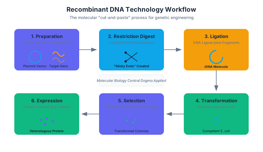
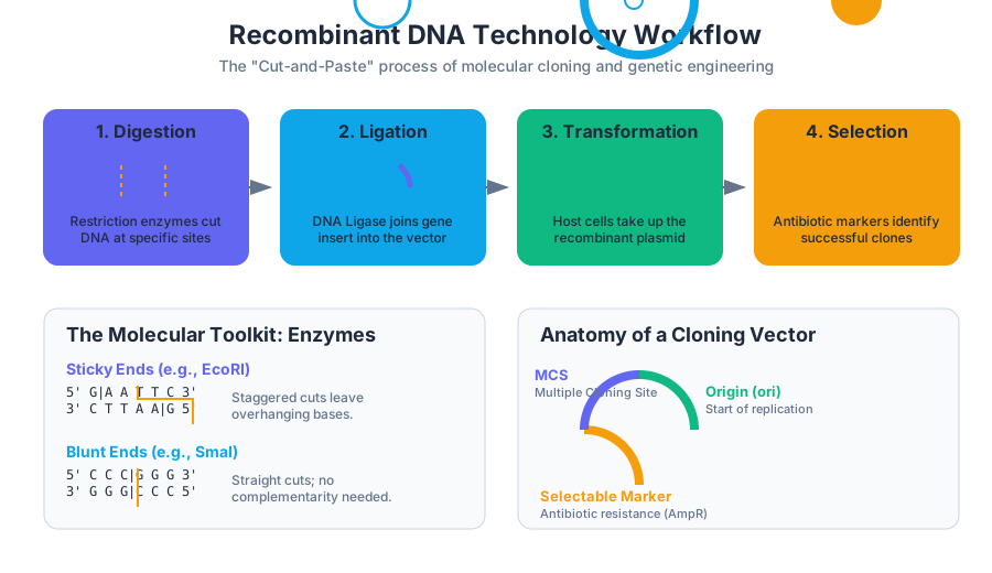
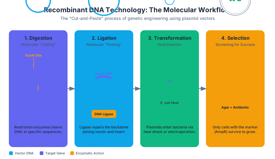
Cell Signaling and Communication

In the complex landscape of multicellular life, the ability of a cell to perceive and respond to its environment is not merely a feature—it is the fundamental requirement for homeostasis, development, and survival. Cell signaling is the biochemical "language" used by cells to coordinate their behavior. At its core, this process involves the conversion of an extracellular signal (a ligand) into a specific intracellular response through a sequence of molecular events known as signal transduction.

This article provides a deep dive into the mechanics of cellular communication, from the thermodynamics of ligand binding to the sophisticated logic gates of kinase cascades.

Ligand-Receptor Interaction: The Initiation of Signal

The signaling process begins with Reception, where a signaling molecule, or ligand, binds to a specific receptor protein. This interaction is governed by the principles of molecular recognition and thermodynamics. Most receptors are transmembrane proteins, possessing an extracellular binding domain and an intracellular signaling domain.

Thermodynamics and Kinetics of Binding

The interaction between a ligand ($L$) and its receptor ($R$) is typically reversible and can be described by the following equilibrium:

R + L \rightleftharpoons RL

The affinity of this interaction is quantified by the dissociation constant ($K_d$), defined as:

$$K_d = \frac{[R][L]}{[RL]}$$

A lower $K_d$ indicates a higher affinity, meaning the receptor can be saturated even at low ligand concentrations. This is crucial in endocrine signaling, where hormones circulate in the blood at nanomolar or picomolar concentrations.

Modes of Signaling

Cells communicate across different distances and through various media. The classification of signaling is based on the distance the ligand travels to reach its target.

Signaling Type	Distance	Mechanism	Example
Endocrine	Long	Ligands (hormones) travel through the bloodstream.	Insulin, Adrenaline
Paracrine	Short	Ligands diffuse through the interstitial fluid to nearby cells.	Neurotransmitters, Growth Factors
Autocrine	Self	The cell secretes a ligand that binds to its own receptors.	T-cell proliferation signals
Juxtacrine	Contact	Signal is transmitted via direct physical contact between cell membranes.	Notch signaling, Gap junctions

Key Insight: The specificity of a cellular response is determined not just by the ligand, but by the specific repertoire of receptors expressed by the target cell and the downstream machinery coupled to those receptors.

---

G-Protein Coupled Receptors (GPCR): The Molecular Switch

GPCRs represent the largest and most diverse group of membrane receptors in eukaryotes. They are characterized by a conserved structure of seven transmembrane (7-TM) alpha-helices. GPCRs act as Guanine Nucleotide Exchange Factors (GEFs) for heterotrimeric G-proteins.

The G-Protein Cycle

A heterotrimeric G-protein consists of three subunits: $\alpha$, $\beta$, and $\gamma$. In its inactive state, the $\alpha$-subunit is bound to GDP.

1. Activation: Ligand binding induces a conformational change in the GPCR, allowing it to bind the G-protein.
2. Exchange: The GPCR triggers the release of GDP from the $G\alpha$ subunit and the binding of GTP.
3. Dissociation: The $G\alpha$-GTP complex dissociates from the $G\beta\gamma$ dimer. Both components can then modulate the activity of downstream effector proteins.
4. Hydrolysis: The $G\alpha$ subunit has intrinsic GTPase activity, eventually hydrolyzing GTP back to GDP, which leads to the re-association of the heterotrimer and termination of the signal.

Low-Level Implementation: G-Protein State Simulation

The following C code demonstrates a simplified state machine representing the transition of a G-protein between active and inactive states, illustrating the "timer" mechanism of intrinsic GTPase activity.

#include <stdio.h>
#include <stdbool.h>

typedef enum { INACTIVE_GDP, ACTIVE_GTP, HYDROLYZING } GProteinState;

typedef struct {
    GProteinState state;
    int intrinsic_gtpase_timer;
    const char* effector_target;
} GProtein;

void process_signal(GProtein *gp, bool ligand_present) {
    switch (gp->state) {
        case INACTIVE_GDP:
            if (ligand_present) {
                printf("GPCR detected ligand: Exchanging GDP for GTP...\n");
                gp->state = ACTIVE_GTP;
                gp->intrinsic_gtpase_timer = 5; // Signal duration
            }
            break;
        case ACTIVE_GTP:
            printf("G-alpha active: Stimulating %s\n", gp->effector_target);
            gp->intrinsic_gtpase_timer--;
            if (gp->intrinsic_gtpase_timer <= 0) {
                gp->state = HYDROLYZING;
            }
            break;
        case HYDROLYZING:
            printf("GTP hydrolyzed to GDP. Reassociating with Beta-Gamma.\n");
            gp->state = INACTIVE_GDP;
            break;
    }
}

int main() {
    GProtein ga_s = {INACTIVE_GDP, 0, "Adenylate Cyclase"};
    bool signal = true;

    for (int i = 0; i < 10; i++) {
        printf("Step %d: ", i);
        process_signal(&ga_s, signal);
        if (i > 2) signal = false; // Ligand dissociates
    }
    return 0;
}

---

Second Messengers: Intracellular Relays

Once a receptor is activated, the signal must be propagated inside the cell. This is often achieved through second messengers—small, non-protein, water-soluble molecules or ions that spread rapidly throughout the cell by diffusion.

Cyclic AMP (cAMP) and the PKA Pathway

One of the most common effectors for GPCRs is Adenylate Cyclase, which converts ATP into cAMP. cAMP typically activates Protein Kinase A (PKA), which then phosphorylates various target proteins to alter cellular metabolism or gene expression.

Phospholipase C (PLC) and Calcium Signaling

Another major pathway involves the activation of Phospholipase C (PLC), which cleaves the membrane phospholipid $PIP_2$ into two distinct second messengers:

1. Inositol trisphosphate ($IP_3$): Diffuses to the Endoplasmic Reticulum (ER) and opens ligand-gated $Ca^{2+}$ channels.
2. Diacylglycerol (DAG): Remains in the membrane and, together with $Ca^{2+}$, activates Protein Kinase C (PKC).

Second Messenger	Origin	Primary Target	Typical Effect
cAMP	ATP (via Adenylate Cyclase)	Protein Kinase A (PKA)	Glycogen breakdown, gene transcription
$IP_3$	$PIP_2$ (via PLC)	$IP_3$-gated $Ca^{2+}$ channels	Release of $Ca^{2+}$ from ER
DAG	$PIP_2$ (via PLC)	Protein Kinase C (PKC)	Cell growth and differentiation
$Ca^{2+}$	ER or extracellular space	Calmodulin, PKC	Muscle contraction, exocytosis

---

Receptor Tyrosine Kinases (RTK) and Kinase Cascades

While GPCRs act as switches, Receptor Tyrosine Kinases (RTKs) function as high-fidelity integrators of growth and differentiation signals. Unlike GPCRs, RTKs have intrinsic enzymatic activity.

Mechanism of RTK Activation

1. Ligand Binding: Two ligands bind to two adjacent RTK monomers.
2. Dimerization: The binding causes the monomers to associate, forming a dimer.
3. Trans-autophosphorylation: The kinase domain of one monomer phosphorylates the tyrosine residues on the cytoplasmic tail of the other monomer.
4. Docking: These phosphorylated tyrosines serve as high-affinity binding sites for intracellular signaling proteins containing SH2 domains.

The MAPK Cascade: A Multi-Stage Amplifier

A classic downstream pathway for RTKs is the Mitogen-Activated Protein Kinase (MAPK) cascade. This involves a sequence of phosphorylation events: Ras (G-protein) -> Raf (MAPKKK) -> MEK (MAPKK) -> ERK (MAPK).

Mathematical Derivation: Signal Amplification Factor

The power of a cascade lies in its ability to amplify a signal exponentially. If each enzyme in a 3-tier cascade activates $n$ molecules of the next tier, the total amplification $A$ is:

A = \prod_{i=1}^{k} n_i

Where:

• $k$ is the number of stages (tiers).
• $n_i$ is the catalytic turnover (amplification) at stage $i$.

Example Derivation: If 1 receptor activates 100 molecules of Enzyme A, and each Enzyme A activates 100 molecules of Enzyme B, and each Enzyme B produces 1000 molecules of product:

1. Stage 1: $1 \times 10^2 = 100$
2. Stage 2: $100 \times 10^2 = 10,000$
3. Stage 3: $10,000 \times 10^3 = 10,000,000$ Total Amplification: $10^7$ (10 million-fold increase from a single binding event).

---

Signal Amplification and Integration

Signal amplification ensures that a minute concentration of an extracellular ligand can trigger a massive cellular response. This is best exemplified by the "Fight or Flight" response mediated by epinephrine.

Quantitative Breakdown of Epinephrine Signaling

The following table illustrates how a single molecule of epinephrine binding to a $\beta$-adrenergic receptor leads to the release of millions of glucose molecules.

Stage	Molecule	Number of Molecules
1	Epinephrine (Ligand)	1
2	Activated GPCR	1
3	Activated $G\alpha_s$	$10^2$
4	Adenylate Cyclase (Effector)	$10^2$
5	cAMP (Second Messenger)	$10^4$
6	Protein Kinase A (PKA)	$10^4$
7	Phosphorylase Kinase	$10^5$
8	Glycogen Phosphorylase	$10^6$
9	Glucose-1-Phosphate	$10^8$

Theorem of Signal Integration: Cells rarely respond to a single signal in isolation. Crosstalk between pathways (e.g., a GPCR pathway inhibiting an RTK pathway) allows the cell to perform complex logic, such as "Only divide if Growth Factor A is present AND Cell Stress B is absent."

---

Termination and Homeostasis

A signal that cannot be turned off is as dangerous as a signal that cannot be turned on (e.g., oncogenic Ras mutations in cancer). Cells employ several mechanisms to terminate signaling:

1. Ligand Dissociation: As extracellular ligand concentration drops, receptors revert to inactive states.
2. GTP Hydrolysis: $G\alpha$ subunits return to the GDP-bound state.
3. Phosphodiesterases (PDE): Enzymes that break down cAMP into AMP, quenching the second messenger signal.
4. Phosphatases: Enzymes that remove phosphate groups from proteins, reversing the action of kinases.
5. Receptor Desensitization: Phosphorylation of the receptor itself can lead to the binding of arrestins, which block further G-protein activation and trigger endocytosis of the receptor.

Real-World Usage: Analyzing Dose-Response with Python

In pharmacology and systems biology, we often model the relationship between ligand concentration and cellular response using the Hill Equation.

import numpy as np
import matplotlib.pyplot as plt
from scipy.optimize import curve_fit

def hill_equation(L, E_max, Kd, n):
    """
    L: Ligand concentration
    E_max: Maximum response
    Kd: Dissociation constant (EC50)
    n: Hill coefficient (cooperativity)
    """
    return E_max * (L**n) / (Kd**n + L**n)

# Simulated experimental data
ligand_conc = np.array([1e-10, 1e-9, 1e-8, 1e-7, 1e-6, 1e-5])
response = np.array([0.02, 0.15, 0.55, 0.88, 0.97, 0.99])

# Fit the model to the data
params, _ = curve_fit(hill_equation, ligand_conc, response)
E_max_fit, Kd_fit, n_fit = params

print(f"Calculated EC50 (Kd): {Kd_fit:.2e} M")
print(f"Hill Coefficient (n): {n_fit:.2f}")

# Visualization
L_plot = np.logspace(-11, -4, 100)
plt.semilogx(L_plot, hill_equation(L_plot, *params), label='Model Fit')
plt.scatter(ligand_conc, response, color='red', label='Data')
plt.xlabel('Ligand Concentration [M]')
plt.ylabel('Normalized Response')
plt.title('Dose-Response Curve Analysis')
plt.legend()
plt.grid(True)
plt.show()

---

Common Pitfalls and Misconceptions

• "Ligands enter the cell": A common mistake is thinking all ligands enter the cell to cause an effect. While steroid hormones (lipophilic) do cross the membrane, the vast majority of ligands (peptides, neurotransmitters) never enter the cytoplasm; they act strictly as "messengers" that knock on the door.
• "Kinases only activate": Phosphorylation is a covalent modification that changes protein conformation. While it often activates enzymes, it can also inhibit them (e.g., phosphorylation of Glycogen Synthase inhibits its activity).
• "One receptor, one effect": A single receptor type can trigger different effects in different tissues depending on the G-proteins and downstream effectors present in those specific cells (e.g., Acetylcholine slows the heart but stimulates skeletal muscle contraction).

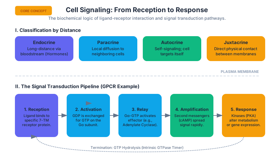
Cell Cycle Regulation and Cancer Biology

The eukaryotic cell cycle is not merely a sequence of growth and division; it is a highly regulated biochemical clockwork designed to ensure the high-fidelity transmission of genetic information. In a multicellular organism, the decision to divide is a collective one, governed by systemic signals and internal checkpoints. When this regulatory architecture collapses, the result is oncogenesis—the transformation of a healthy cell into a malignant one. This article explores the molecular mechanics of the cell cycle engine, the surveillance systems that guard it, and the genetic failures that lead to cancer.

The Molecular Engine: Cyclins and Cdks

At the heart of the cell cycle is a family of serine/threonine kinases known as Cyclin-Dependent Kinases (Cdks). These enzymes are the "engines" of the cell cycle, but they are intrinsically inactive. They require the binding of a regulatory subunit called a Cyclin to achieve catalytic competence.

The Logic of Oscillating Activity

The cell cycle progresses through four distinct phases: G1 (Gap 1), S (Synthesis), G2 (Gap 2), and M (Mitosis). The concentration of Cdks remains relatively constant throughout the cycle, but the concentration of Cyclins oscillates dramatically. This oscillation is driven by periodic transcription and rapid, irreversible degradation via the Ubiquitin-Proteasome System (UPS).

Definition: The Cyclin-Cdk Complex A heterodimeric protein complex where the Cyclin subunit provides substrate specificity and the Cdk subunit provides the kinase activity. The activation of the complex typically requires phosphorylation of the "T-loop" by a Cdk-Activating Kinase (CAK).

Phase	Cyclin	Cdk Partner	Primary Function
G1	Cyclin D (D1, D2, D3)	Cdk4, Cdk6	Responding to extracellular growth factors; initiating G1.
G1/S	Cyclin E	Cdk2	Triggering the "Restriction Point"; preparing for DNA replication.
S	Cyclin A	Cdk2, Cdk1	Initiating DNA synthesis; ensuring single replication per cycle.
M	Cyclin B	Cdk1	Triggering nuclear envelope breakdown and spindle assembly.

Regulation of Cdk Activity

Cdk activity is controlled by three primary mechanisms:

1. Cyclin Availability: Controlled by synthesis and degradation (e.g., APC/C and SCF ubiquitin ligases).
2. Inhibitory Phosphorylation: The kinases Wee1 and Myt1 phosphorylate Cdk1 at Tyr15 and Thr14, inhibiting it. The phosphatase Cdc25 removes these phosphates to trigger entry into mitosis.
3. Cdk Inhibitors (CKIs): Proteins like p21, p27, and p16 bind directly to the complex to physically block activity.

/* 
 * Low-level simulation of a Cdk1 State Machine 
 * This C represents the biochemical "logic gate" of the M-phase entry.
 */

#include <stdio.h>
#include <stdbool.h>

typedef struct {
    bool cyclin_b_bound;
    bool thr161_phosphorylated; // Activating
    bool tyr15_phosphorylated;  // Inhibitory
    bool p21_bound;             // CKI
} Cdk1_Complex;

bool is_cdk1_active(Cdk1_Complex *complex) {
    // Logic: Must have cyclin, must be activated by CAK, 
    // must NOT be inhibited by Wee1, must NOT be bound by CKI.
    return (complex->cyclin_b_bound && 
            complex->thr161_phosphorylated && 
            !complex->tyr15_phosphorylated && 
            !complex->p21_bound);
}

int main() {
    Cdk1_Complex m_phase_entry = {true, true, false, false};
    if (is_cdk1_active(&m_phase_entry)) {
        printf("Cell entering Mitosis: MPF active.\n");
    }
    return 0;
}

The Restriction Point and the RB/E2F Pathway

The most critical decision a cell makes is whether to exit G1 and enter S-phase. This transition is known as the Restriction Point (R-point). Before this point, the cell requires external mitogens (growth factors) to proceed. After the R-point, the cell is committed to division even if growth factors are withdrawn.

The RB/E2F Switch

The R-point is governed by the Retinoblastoma protein (RB), a tumor suppressor. In its unphosphorylated state, RB binds to the transcription factor E2F, effectively sequestering it and preventing the expression of genes required for S-phase (such as DNA polymerase and Cyclin E).

The Mechanism of Release:

1. Mitogen Signaling: Growth factors trigger the synthesis of Cyclin D.
2. Hypo-phosphorylation: Cyclin D-Cdk4/6 complexes phosphorylate RB at a few sites.
3. Hyper-phosphorylation: This initial phosphorylation allows Cyclin E-Cdk2 to further phosphorylate RB, leading to a conformational change.
4. E2F Release: Hyper-phosphorylated RB releases E2F.
5. Positive Feedback: E2F promotes the transcription of more Cyclin E and its own gene, creating a "bistable switch" that locks the cell into S-phase entry.

Mathematical Modeling of the G1/S Switch

The transition from G1 to S is often modeled as a sigmoidal response. The concentration of active E2F ($[E2F]$) relative to the concentration of Cyclin D ($[CycD]$) can be described by a Hill equation, representing the cooperative nature of the feedback loops.

\frac{d[E2F]}{dt} = \frac{k_s [CycD]^n}{K_m^n + [CycD]^n} - k_d [E2F]

Where:

• $k_s$ is the synthesis rate constant.
• $k_d$ is the degradation rate constant.
• $n$ is the Hill coefficient (indicating the "steepness" of the switch).
• $K_m$ is the threshold concentration for activation.

Surveillance Systems: Checkpoints and p53

Checkpoints are quality-control mechanisms that pause the cell cycle if specific conditions are not met. The most famous of these is the DNA Damage Checkpoint, mediated by the "Guardian of the Genome," p53.

The p53-MDM2 Feedback Loop

Under normal conditions, p53 levels are kept extremely low by MDM2, an E3 ubiquitin ligase that targets p53 for degradation. When DNA damage occurs (e.g., double-strand breaks), kinases like ATM or ATR are activated. These kinases phosphorylate p53, preventing its interaction with MDM2.

The p53 Response Pipeline:

1. Detection: ATM/ATR sense DNA lesions.
2. Stabilization: p53 is phosphorylated and stabilized.
3. Transcriptional Activation: p53 acts as a tetrameric transcription factor for:
   • p21 (WAF1/CIP1): A CKI that halts the cell cycle in G1 by inhibiting Cyclin E-Cdk2.
   • GADD45: Involved in DNA repair.
   • BAX/PUMA: Pro-apoptotic factors (if damage is irreparable).

Cancer Biology: The Failure of Control

Cancer is fundamentally a genetic disease characterized by the accumulation of mutations in genes that regulate the cell cycle. These mutations fall into two broad categories: Proto-oncogenes and Tumor Suppressors.

Proto-oncogenes vs. Tumor Suppressors

A Proto-oncogene is a normal gene that promotes cell growth. When mutated into an Oncogene, it gains function (is "always on"). A Tumor Suppressor is a gene that inhibits growth or repairs DNA. It must lose function (usually in both alleles) to contribute to cancer.

Feature	Proto-oncogene	Tumor Suppressor
Normal Function	Promotes division/survival	Inhibits division/promotes apoptosis
Mutation Type	Gain-of-function (Dominant)	Loss-of-function (Recessive)
Analogy	Stuck Accelerator	Broken Brakes
Example	Ras, HER2, MYC	TP53, RB1, BRCA1

The "Two-Hit" Hypothesis

Proposed by Alfred Knudson, this hypothesis explains why certain cancers are hereditary. In hereditary retinoblastoma, a child inherits one defective copy of the RB1 gene (the first "hit"). They only need one somatic mutation in the second allele (the second "hit") in any retinal cell to develop a tumor. In sporadic cases, both hits must occur in the same cell lineage, which is statistically much rarer.

Case Study: The Ras Pathway

The Ras protein is a small GTPase that acts as a molecular switch in the growth factor signaling pathway.

• Active State: Ras-GTP (promotes growth).
• Inactive State: Ras-GDP.
• Oncogenic Mutation: Most Ras mutations (e.g., G12V) inhibit the intrinsic GTPase activity, meaning Ras cannot turn itself off. It remains in the GTP-bound state, constantly signaling the cell to divide regardless of external signals.

# Analyzing mutation frequency in a hypothetical cancer genomics dataset
import pandas as pd

# Mock data: Gene mutation counts across 1000 tumor samples
data = {
    'Gene': ['TP53', 'KRAS', 'RB1', 'PTEN', 'MYC', 'BRCA1'],
    'Mutation_Type': ['TS', 'OG', 'TS', 'TS', 'OG', 'TS'], # TS=Tumor Suppressor, OG=Oncogene
    'Frequency': [0.52, 0.28, 0.15, 0.12, 0.22, 0.05]
}

df = pd.DataFrame(data)

# Calculate the ratio of TS vs OG mutations in high-frequency drivers (>20%)
high_freq = df[df['Frequency'] > 0.20]
summary = high_freq.groupby('Mutation_Type').size()

print("High-Frequency Driver Analysis:")
print(summary)
print(f"\nPrimary Driver: {df.iloc[df['Frequency'].idxmax()]['Gene']}")

Apoptosis: The Programmed Exit

When a cell's internal monitoring systems detect catastrophic failure (e.g., massive DNA damage or viral infection), it initiates Apoptosis—programmed cell death. This is a clean, ATP-dependent process that avoids the inflammatory response associated with necrosis.

The Caspase Cascade

Apoptosis is executed by Caspases (Cysteine-aspartic proteases). They exist as inactive pro-caspases and are activated through proteolytic cleavage.

1. Intrinsic Pathway (Mitochondrial): Triggered by internal stress. The mitochondria release Cytochrome c into the cytosol, which binds to Apaf-1 to form the Apoptosome. This activates Caspase-9.
2. Extrinsic Pathway (Death Receptor): Triggered by external signals (e.g., Fas ligand). This activates Caspase-8.
3. Execution: Both pathways converge on Caspase-3, which cleaves structural proteins and activates DNases to fragment the genome.

The Bcl-2 Family: The Rheostat of Life

The decision to undergo apoptosis is governed by the ratio of pro-apoptotic to anti-apoptotic proteins in the Bcl-2 family.

Protein Group	Members	Function
Anti-apoptotic	Bcl-2, Bcl-xL	Sequestration of pro-apoptotic factors; stabilizing the mitochondria.
Pro-apoptotic (Effector)	BAX, BAK	Forming pores in the mitochondrial outer membrane (MOMP).
Pro-apoptotic (BH3-only)	PUMA, NOXA, Bad	Sensing stress and neutralizing anti-apoptotic members.

Key Insight: The Warburg Effect Cancer cells often exhibit altered metabolism, favoring glycolysis even in the presence of oxygen. This "Aerobic Glycolysis" provides the carbon skeletons necessary for rapid biomass accumulation (nucleotides, lipids) required for continuous cell division.

Therapeutic Strategies

Understanding the cell cycle has led to the development of targeted therapies that exploit the specific vulnerabilities of cancer cells.

1. Cdk4/6 Inhibitors: Drugs like Palbociclib are used in ER-positive breast cancer to prevent RB phosphorylation, effectively "locking" the cancer cells in G1.
2. PARP Inhibitors: Used in BRCA-mutant cancers. Since these cells already lack one DNA repair pathway, inhibiting a second pathway (PARP) leads to "Synthetic Lethality"—the cell accumulates too much damage to survive.
3. Immunotherapy: Using checkpoint inhibitors (e.g., Anti-PD-1) to prevent cancer cells from "turning off" the immune system's T-cells.

Common Pitfalls and Misconceptions

• "Cdk levels change": A common mistake. Cdk protein levels are generally stable; it is the Cyclin levels and Cdk phosphorylation state that change.
• "p53 always causes death": p53 first attempts to trigger G1 arrest and DNA repair. Apoptosis is the final resort if repair fails.
• "One mutation causes cancer": Cancer is a multi-step process. It typically requires 5–7 major "driver" mutations in different pathways (growth, apoptosis, immortality, angiogenesis) to become a fully malignant tumor.

Neurobiology and Optogenetics

The nervous system represents the most complex biological computational engine known. At its core, neurobiology is the study of how cells—specifically neurons—utilize electrochemical gradients to process, store, and transmit information. This section delves into the biophysical mechanisms of neural signaling, the molecular machinery of the synapse, and the transformative technology of optogenetics, which allows for the precise interrogation of neural circuits using light.

The Biophysics of the Resting Membrane Potential

Before a neuron can fire, it must establish a state of readiness. This is the Resting Membrane Potential (RMP), typically measured at approximately -70 mV. This potential is not merely a "static" charge but a dynamic equilibrium maintained by the selective permeability of the lipid bilayer and the active transport of ions.

The Ionic Gradient and the Na+/K+ Pump

The lipid bilayer, as discussed in previous biochemical contexts, is impermeable to ions. Therefore, neurons rely on specialized transmembrane proteins. The most critical is the Na+/K+-ATPase (Sodium-Potassium Pump).

The 3:2 Ratio: For every three $Na^+$ ions pumped out of the cell, two $K^+$ ions are pumped in, consuming one molecule of ATP. This creates a net loss of positive charge inside the cell and establishes a steep concentration gradient.

Ion	Intracellular Conc. (mM)	Extracellular Conc. (mM)	Relative Permeability (Rest)
$K^+$	140	5	1.0
$Na^+$	5–15	145	0.04
$Cl^-$	4–30	110	0.45
$Ca^{2+}$	0.0001	1–2	Very Low

The Nernst and GHK Equations

To calculate the equilibrium potential for a single ion, we use the Nernst Equation. However, because the membrane is permeable to multiple ions simultaneously, the actual membrane potential ($V_m$) is determined by the Goldman-Hodgkin-Katz (GHK) Equation.

V_m = \frac{RT}{F} \ln \left( \frac{P_{K}[K^+]_{out} + P_{Na}[Na^+]_{out} + P_{Cl}[Cl^-]_{in}}{P_{K}[K^+]_{in} + P_{Na}[Na^+]_{in} + P_{Cl}[Cl^-]_{out}} \right)

Where:

• $R$ is the universal gas constant.
• $T$ is the absolute temperature (Kelvin).
• $F$ is Faraday's constant.
• $P_x$ is the permeability of ion $x$.

The Action Potential: The Digital Pulse of Life

The Action Potential (AP) is an "all-or-none" electrochemical event. When a neuron's membrane potential reaches a specific threshold (typically -55 mV), it triggers a rapid reversal of charge.

Mechanics of the Voltage-Gated Ion Channel

The AP is driven by voltage-gated ion channels. These proteins contain a voltage-sensing domain (usually S4 alpha-helices with positively charged residues) that shifts in response to depolarization, opening the pore.

1. Depolarization: Voltage-gated $Na^+$ channels open rapidly. $Na^+$ rushes into the cell, driven by both the concentration gradient and the negative internal charge.
2. Peak: The membrane potential reaches roughly +30 to +40 mV. At this point, $Na^+$ channels enter an inactivated state (the "ball-and-chain" mechanism).
3. Repolarization: Slower voltage-gated $K^+$ channels open. $K^+$ flows out of the cell, restoring the negative internal charge.
4. Hyperpolarization: $K^+$ channels stay open slightly too long, moving the potential closer to the $K^+$ equilibrium potential (-90 mV) than the resting state.

The Hodgkin-Huxley Model

In 1952, Alan Hodgkin and Andrew Huxley published a set of differential equations describing how these currents behave. This remains the gold standard for computational neuroscience.

import numpy as np
import matplotlib.pyplot as plt

# Hodgkin-Huxley Model Simulation
def simulate_hh_model(t_max=50, dt=0.01, I_ext=10.0):
    # Constants (Conductance in mS/cm^2, Capacitance in uF/cm^2, Potential in mV)
    C_m = 1.0
    g_Na, g_K, g_L = 120.0, 36.0, 0.3
    E_Na, E_K, E_L = 50.0, -77.0, -54.387

    # Alpha/Beta functions for gating variables
    def alpha_m(V): return 0.1 * (V + 40.0) / (1.0 - np.exp(-(V + 40.0) / 10.0))
    def beta_m(V):  return 4.0 * np.exp(-(V + 65.0) / 18.0)
    def alpha_h(V): return 0.07 * np.exp(-(V + 65.0) / 20.0)
    def beta_h(V):  return 1.0 / (1.0 + np.exp(-(V + 35.0) / 10.0))
    def alpha_n(V): return 0.01 * (V + 55.0) / (1.0 - np.exp(-(V + 55.0) / 10.0))
    def beta_n(V):  return 0.125 * np.exp(-(V + 65.0) / 80.0)

    t = np.arange(0, t_max, dt)
    V = np.zeros_like(t)
    m, h, n = np.zeros_like(t), np.zeros_like(t), np.zeros_like(t)

    # Initial states
    V[0] = -65.0
    m[0], h[0], n[0] = 0.05, 0.6, 0.32

    for i in range(1, len(t)):
        # Calculate currents
        I_Na = g_Na * (m[i-1]**3) * h[i-1] * (V[i-1] - E_Na)
        I_K = g_K * (n[i-1]**4) * (V[i-1] - E_K)
        I_L = g_L * (V[i-1] - E_L)
        
        # Update V
        dV = (I_ext - I_Na - I_K - I_L) / C_m
        V[i] = V[i-1] + dV * dt
        
        # Update gating variables using Euler method
        m[i] = m[i-1] + (alpha_m(V[i-1])*(1-m[i-1]) - beta_m(V[i-1])*m[i-1]) * dt
        h[i] = h[i-1] + (alpha_h(V[i-1])*(1-h[i-1]) - beta_h(V[i-1])*h[i-1]) * dt
        n[i] = n[i-1] + (alpha_n(V[i-1])*(1-n[i-1]) - beta_n(V[i-1])*n[i-1]) * dt

    return t, V

# Example usage:
# time, voltage = simulate_hh_model(I_ext=15.0)

Synaptic Transmission: Chemical Computation

When the action potential reaches the axon terminal, the electrical signal must be converted into a chemical one to cross the synaptic cleft (a ~20nm gap).

The Mechanism of Vesicle Release

1. Calcium Influx: The arrival of the AP depolarizes the terminal, opening Voltage-Gated Calcium Channels (VGCCs).
2. Exocytosis: $Ca^{2+}$ ions bind to synaptotagmin, a protein on the surface of neurotransmitter-filled vesicles. This triggers the SNARE complex to fuse the vesicle membrane with the terminal membrane.
3. Diffusion: Neurotransmitters spill into the cleft and bind to receptors on the post-synaptic membrane.

Neurotransmitters and Receptors

Neurotransmitters are classified by their effect on the post-synaptic neuron:

• Excitatory (EPSP): Lead to depolarization (e.g., Glutamate opening $Na^+$ channels).
• Inhibitory (IPSP): Lead to hyperpolarization (e.g., GABA opening $Cl^-$ channels).

Class	Examples	Primary Receptor Type	Major Function
Amino Acids	Glutamate, GABA, Glycine	Ionotropic & Metabotropic	Fast signaling, Inhibition
Biogenic Amines	Dopamine, Serotonin, NE	Mostly Metabotropic (GPCR)	Neuromodulation, Mood
Neuropeptides	Endorphins, Substance P	Metabotropic	Pain, Reward
Gases	Nitric Oxide (NO)	Diffusion	Retrograde signaling

Optogenetics: Controlling Circuits with Light

Traditional methods of brain stimulation (like electrical microstimulation) are "blunt instruments"—they activate all cell types in a given area. Optogenetics solves this by using genetic engineering to express light-sensitive ion channels in specific populations of neurons.

The Microbial Opsins

The foundation of optogenetics lies in microbial proteins called opsins. Unlike the opsins in our eyes, which trigger complex signaling cascades, microbial opsins are single-component systems: the light sensor and the ion channel are the same protein.

1. Channelrhodopsin-2 (ChR2): Derived from green algae (Chlamydomonas reinhardtii). Responds to blue light (~470nm) by opening a cation channel, allowing $Na^+$ influx and causing depolarization (activation).
2. Halorhodopsin (NpHR): Derived from archaea (Natronomonas pharaonis). Responds to yellow light (~580nm) by pumping $Cl^-$ ions into the cell, causing hyperpolarization (silencing).
3. Archaerhodopsin (Arch): An outward proton pump that silences neurons in response to green/yellow light.

Implementation Pipeline

To use optogenetics in a research setting, a specific workflow is followed:

1. Genetic Targeting: A viral vector (like AAV) carrying the opsin gene is injected into a specific brain region. The gene is often placed under a cell-type-specific promoter (e.g., the CaMKIIa promoter for excitatory neurons).
2. Light Delivery: An optical fiber is chronically implanted into the brain, connected to a laser or LED source.
3. Behavioral Interrogation: The researcher pulses light while observing behavior, allowing for a causal link between specific neural activity and specific actions.

# Optogenetic Experimental Configuration Example
experiment_metadata:
  subject_id: "Mice-Line-TH-Cre-042"
  brain_region: "Ventral Tegmental Area (VTA)"
  opsin:
    name: "ChR2-mCherry"
    vector: "AAV5-EF1a-DIO-hChR2(H134R)-mCherry"
    activation_wavelength: 473nm # Blue light
  stimulation_protocol:
    frequency: 20Hz
    pulse_width: 5ms
    duty_cycle: 10%
    power_at_tip: 10mW
  behavioral_task: "Real-time Place Preference (RTPP)"

Advanced Considerations and Pitfalls

Temporal vs. Spatial Precision

While optogenetics offers millisecond-scale temporal precision, it faces challenges in spatial scattering. Light loses intensity as it travels through brain tissue.

The Scattering Equation: $I(z) = I_0 \cdot e^{-\mu_s z}$, where $\mu_s$ is the scattering coefficient of the tissue. In the brain, blue light scatters much more than red light, which is why researchers are developing "red-shifted" opsins for deeper penetration.

Common Pitfalls in Neurobiology

• Assuming "Activation" equals "Function": Just because stimulating a neuron causes a behavior doesn't mean that neuron is the only or primary cause of that behavior in nature.
• Heat Artifacts: High-intensity laser light can heat the brain tissue, potentially altering the firing rates of neurons independently of the opsins.
• Overexpression: Too much opsin can lead to "leaky" membranes or cell death (phototoxicity).

Hardware Control: Pulse Width Modulation (PWM)

In a laboratory rig, controlling the light source requires precise timing. Below is a low-level example of how a microcontroller (like an Arduino or STM32) might handle the timing for a 20Hz stimulation.

/* 
 * Low-level Optogenetic Stimulator Control (C)
 * Target: AVR-based Microcontroller (e.g., ATmega328P)
 * Purpose: Generate precise 20Hz pulses with 5ms duration
 */

#include <avr/io.h>
#include <util/delay.h>

#define LASER_PIN PB1 // Digital Pin 9 on Arduino

void setup_timer() {
    // Set PB1 as output
    DDRB |= (1 << LASER_PIN);
}

void trigger_pulse(int frequency_hz, int duration_ms, int total_seconds) {
    int period_ms = 1000 / frequency_hz;
    int off_time_ms = period_ms - duration_ms;
    int total_pulses = frequency_hz * total_seconds;

    for (int i = 0; i < total_pulses; i++) {
        PORTB |= (1 << LASER_PIN);  // Laser ON
        _delay_ms(duration_ms);     // Wait for pulse width
        
        PORTB &= ~(1 << LASER_PIN); // Laser OFF
        _delay_ms(off_time_ms);    // Wait for remainder of period
    }
}

int main(void) {
    setup_timer();
    while(1) {
        // Example: 20Hz, 5ms pulse, for 10 seconds
        trigger_pulse(20, 5, 10);
        _delay_ms(5000); // 5 second rest between trials
    }
}

Summary of Neuro-Engineering Tools

The evolution of neurobiology has moved from observation to manipulation. The table below compares the primary methods of neural interrogation.

Method	Spatial Resolution	Temporal Resolution	Cell-Type Specificity	Invasiveness
fMRI	Low (mm)	Very Low (sec)	None	Non-invasive
EEG	Very Low (cm)	High (ms)	None	Non-invasive
Microstimulation	Medium (um)	High (ms)	None	Invasive
Optogenetics	High (um)	Very High (ms)	Very High	Invasive
Chemogenetics (DREADDs)	High (um)	Low (min/hours)	Very High	Invasive (Viral)

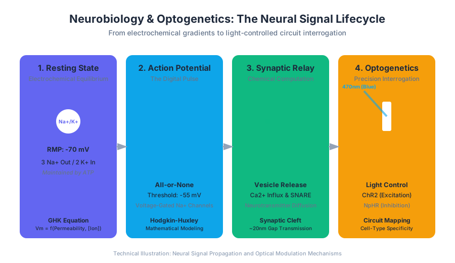
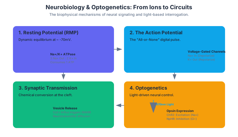
Immunology and Molecular Applications

The mammalian immune system is perhaps the most complex decentralized computing network in existence. It must solve a multi-variable optimization problem: identifying an almost infinite variety of evolving pathogens ("non-self") while maintaining absolute tolerance toward the host's own tissues ("self"). This section explores the molecular architecture of this system—from the genomic rearrangements that generate diversity to the high-throughput technologies, such as DNA microarrays, that allow us to observe these processes at a systems level.

The Architecture of Adaptive Immunity: B and T Cells

The immune system is bifurcated into Innate and Adaptive responses. While the innate system provides immediate, non-specific defense via pattern recognition receptors (PRRs), the adaptive system relies on the exquisite specificity of Lymphocytes: B cells and T cells.

B Cells and Humoral Immunity

B Lymphocytes are the mediators of humoral immunity. Their primary function is the production of Antibodies (Immunoglobulins, Ig). Each B cell is genetically programmed to produce a single type of antibody. When a B cell encounters its cognate antigen, it undergoes clonal expansion and differentiates into plasma cells (antibody factories) and memory cells.

T Cells and Cell-Mediated Immunity

T Lymphocytes do not recognize free-floating antigens. Instead, they recognize processed peptide fragments presented on the surface of other cells.

• Helper T Cells (CD4+): Coordinate the immune response by secreting cytokines. They recognize antigens presented by MHC Class II molecules.
• Cytotoxic T Cells (CD8+): Directly kill infected or cancerous cells. They recognize antigens presented by MHC Class I molecules.

Feature	B Cells	T Cells
Site of Maturation	Bone Marrow	Thymus
Antigen Receptor	B-Cell Receptor (BCR) / Antibody	T-Cell Receptor (TCR)
Antigen Recognition	Soluble/Free Antigens	Processed peptides on MHC
Effector Function	Antibody Secretion	Cytolysis, Cytokine Production
Memory	Yes	Yes

The Molecular Structure of Recognition: Antibodies and MHC

The specificity of the immune response is governed by the structural complementarity between the receptor and the ligand.

Antibody Structure

An antibody is a Y-shaped tetrameric glycoprotein consisting of two identical Heavy (H) chains and two identical Light (L) chains.

• Variable (V) Regions: Located at the tips of the "Y," these form the Antigen-Binding Site (Paratope).
• Constant (C) Regions: Determine the antibody's isotype (IgG, IgM, IgE, IgA, IgD) and its effector functions (e.g., crossing the placenta, activating complement).

The Affinity Constant ($K_a$): The strength of the interaction between an antibody and its antigen is defined by the equilibrium association constant: $$K_a = \frac{[Ab-Ag]}{[Ab][Ag]}$$ High-affinity antibodies typically have a $K_d$ (dissociation constant) in the range of $10^{-9}$ to $10^{-12}$ M.

The Major Histocompatibility Complex (MHC)

MHC molecules are the "display cases" of the cell. They are highly polymorphic, meaning there is immense variation between individuals, which is why organ transplant rejection occurs.

MHC Class	Expression Pattern	Source of Peptide	Recognized By
Class I	All nucleated cells	Endogenous (Cytosol/Viruses)	CD8+ T Cells
Class II	Professional APCs (Dendritic cells, Macrophages, B cells)	Exogenous (Phagocytosed)	CD4+ T Cells

VDJ Recombination: Generating Infinite Diversity from Finite DNA

One of the most profound questions in 20th-century biology was how the genome, which contains only ~20,000 genes, could encode billions of unique antibody specificities. The answer, discovered by Susumu Tonegawa, is Somatic Recombination.

The Mechanism

In germline DNA, the gene segments for the variable regions of antibodies are stored in "libraries" of segments: Variable (V), Diversity (D), and Joining (J).

1. Recombination Activating Genes (RAG-1 and RAG-2) recognize specific DNA sequences called Recombination Signal Sequences (RSS).
2. The RAG complex introduces double-strand breaks at the edges of the V, D, and J segments.
3. The intervening DNA is excised, and the segments are ligated together by Non-Homologous End Joining (NHEJ).

The Mathematics of Diversity

The total potential diversity of the primary antibody repertoire is the product of several factors:

• Combinatorial Diversity: $V \times D \times J$ combinations.
• Junctional Diversity: The imprecise joining of segments, where nucleotides (P-nucleotides and N-nucleotides) are added or deleted by the enzyme TdT (Terminal Deoxynucleotidyl Transferase).
• Chain Pairing: The random combination of one Heavy chain and one Light chain.

# A simplified simulation of combinatorial diversity in the Human Heavy Chain
import itertools

def calculate_diversity():
    # Approximate counts of functional gene segments in humans
    v_segments = 40
    d_segments = 25
    j_segments = 6
    
    # Combinatorial possibilities for the Heavy Chain
    heavy_combinations = v_segments * d_segments * j_segments
    
    # Light Chain (Kappa and Lambda)
    # Kappa: V(~35) * J(5) | Lambda: V(~30) * J(4)
    light_combinations = (35 * 5) + (30 * 4)
    
    # Total combinatorial diversity (Heavy x Light)
    total_combinatorial = heavy_combinations * light_combinations
    
    print(f"Heavy Chain Combinations: {heavy_combinations}")
    print(f"Light Chain Combinations: {light_combinations}")
    print(f"Total Combinatorial Diversity: {total_combinatorial:.2e}")
    
    # Note: Junctional diversity adds a factor of ~10^7 to 10^11
    junctional_multiplier = 10**10
    print(f"Estimated Total Diversity with Junctional Effects: {total_combinatorial * junctional_multiplier:.2e}")

calculate_diversity()

Somatic Hypermutation and Affinity Maturation

After a B cell is activated by an antigen, it migrates to a germinal center in a lymph node. There, it undergoes Somatic Hypermutation (SHM). The enzyme AID (Activation-Induced Cytidine Deaminase) introduces mutations into the V regions at a rate $10^6$ times higher than the background mutation rate.

Cells with mutations that increase affinity for the antigen are "selected" to survive, while those with lower affinity undergo apoptosis. This iterative process is known as Affinity Maturation, a biological implementation of a genetic algorithm.

\text{Probability of improved affinity } P(\Delta A > 0) = \int_{S} f(m) \cdot w(m) \, dm

Where $f(m)$ is the distribution of mutations $m$, and $w(m)$ is the fitness weight of that mutation in the context of antigen binding.

Molecular Applications: DNA Microarrays

While immunology focuses on the body's natural defenses, Molecular Applications use these principles (specifically nucleic acid hybridization and antibody specificity) to create diagnostic and research tools.

DNA Microarray Mechanics

A DNA microarray (or "gene chip") is a solid surface (glass or silicon) onto which thousands of microscopic spots of DNA (probes) are attached. Each spot contains a specific DNA sequence representing a gene.

1. RNA Extraction: Total RNA is extracted from two samples (e.g., Healthy vs. Cancerous tissue).
2. Reverse Transcription: RNA is converted to cDNA.
3. Labeling: cDNA from the healthy sample is labeled with a green fluorophore (Cy3), and the cancer sample with a red fluorophore (Cy5).
4. Hybridization: The labeled samples are mixed and washed over the microarray. cDNA strands bind (hybridize) to their complementary probes.
5. Scanning: A laser excites the fluorophores, and the ratio of Red to Green (R/G) is measured.

Resulting Color	Interpretation	Expression Ratio (Cy5/Cy3)
Red	Gene upregulated in experimental sample	$> 1$
Green	Gene downregulated in experimental sample	$< 1$
Yellow	Equal expression in both samples	$\approx 1$
Black	Gene not expressed in either sample	$0$

Data Processing and Normalization

Raw microarray data is noisy. We use the Log-Ratio to handle the data, as it treats up-regulation and down-regulation symmetrically.

# Example workflow for processing Microarray data using a CLI tool like 'limma' in R
# 1. Load the target file describing the samples
# 2. Read the intensities from the scanner output (e.g., GenePix .gpr files)
# 3. Background correction and normalization (Loess normalization)
# 4. Fit a linear model to identify Differentially Expressed Genes (DEGs)

Rscript -e "
library(limma);
targets <- readTargets('targets.txt');
RG <- read.maimages(targets, source='genepix');
RG_norm <- normalizeWithinArrays(RG, method='loess');
fit <- lmFit(RG_norm, design=c(1,1,-1,-1)); # Example 2 vs 2 design
fit <- eBayes(fit);
topTable(fit);
"

Advanced Molecular Tools: Monoclonal Antibodies and GFP

The specificity of the immune system has been "harnessed" for biotechnology.

Monoclonal Antibodies (mAbs)

Produced via Hybridoma Technology, monoclonal antibodies are identical immune cells that are clones of a single parent cell.

• Process: Fuse a B cell (producing the desired antibody) with a myeloma cell (a cancerous B cell that is "immortal").
• Applications: Targeted cancer therapies (e.g., Herceptin), diagnostic assays (ELISA), and neutralizing viral infections.

Green Fluorescent Protein (GFP)

Originally isolated from the jellyfish Aequorea victoria, GFP is a tool for visualizing protein localization in live cells. By fusing the DNA sequence of GFP to a gene of interest, researchers can "tag" proteins and track their movement using fluorescence microscopy.

Common Pitfalls and Technical Nuances

1. Cross-Reactivity: An antibody may bind to an epitope that is structurally similar to its intended target. This is a major source of "noise" in ELISAs and can lead to autoimmune diseases (e.g., Rheumatic fever).
2. MHC Restriction: A T cell will only recognize a peptide if it is presented on the specific MHC molecule that the T cell "learned" on during its development in the thymus.
3. Microarray vs. RNA-Seq: While microarrays are cost-effective for known genomes, they cannot discover new genes or splice variants. RNA-Seq (Next-Generation Sequencing) has largely superseded microarrays for discovery-based research because it provides absolute quantification and higher dynamic range.

Feature	DNA Microarray	RNA-Seq (NGS)
Principle	Hybridization	Sequencing
Requirement	Prior knowledge of sequence	No prior knowledge needed
Dynamic Range	Limited ($10^2 - 10^3$)	High ($10^5 +$)
Cost	Lower	Higher (though falling)

Summary of the Molecular Pipeline

The journey from a pathogen encounter to a molecular diagnostic tool involves a series of highly regulated steps:

1. Recognition: B/T cells identify the pathogen via VDJ-generated receptors.
2. Expansion: Clonal selection amplifies the specific responders.
3. Optimization: Somatic hypermutation refines antibody affinity.
4. Observation: We use tools like Microarrays and Monoclonal antibodies to measure and mimic these natural processes for human health.

Through the integration of genetics, biochemistry, and engineering, immunology has transitioned from a descriptive medical field to a precise molecular science.