Introduction to Computer Science and Programming in Python
Institution: MIT
64 study materials · 12 sections
MIT's 6.0001 Introduction to Computer Science and Programming in Python is a foundational course designed for students with little to no prior programming experience. The course focuses on using Python 3.5 to develop computational problem-solving skills, blending the creativity of algorithm design with the logic of implementation. Students learn to write small, effective programs through a curriculum that covers basic control flow, data structures, and software engineering principles like testing and debugging.
Course Sections
Introduction to Computational Thinking
Key concepts: Algorithm fundamentals · Growth mindset · Active learning · Creativity vs. Logic · Rubber Ducking
Explores the philosophy of programming as a foundational skill and the mindset required for effective problem-solving.
Introduction to Computational Thinking
Computational thinking is the conceptual foundation of modern problem-solving. It is not merely the act of writing code in a specific programming language like Python or C++; rather, it is a high-level mental framework used to decompose complex problems into discrete, manageable steps that a processing agent (human or machine) can execute. As a discipline, it sits at the intersection of mathematical logic and creative engineering.
The Nature of Computation: Declarative vs. Imperative
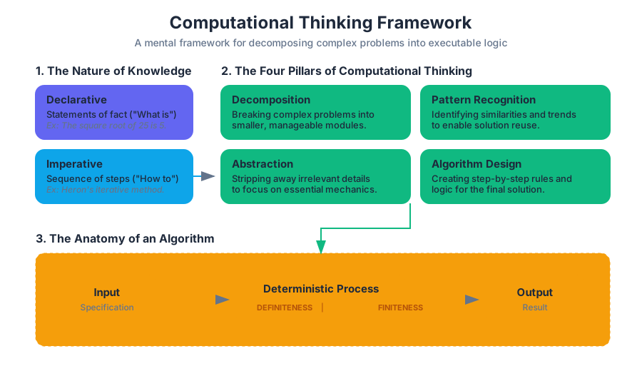
To understand computational thinking, one must first distinguish between two fundamental types of knowledge: Declarative and Imperative.
- Declarative Knowledge consists of statements of fact. It describes "what is." For example, the statement "The square root of a number $x$ is a number $y$ such that $y \cdot y = x$" is declarative. It defines the relationship but provides no instructions on how to find $y$.
- Imperative Knowledge is a "how-to" description. It is a sequence of steps—an algorithm—that leads to a result. To find a square root imperatively, one might use Heron's method (an iterative approximation).
Definition: Algorithm An algorithm is a finite, deterministic sequence of instructions where each step is precisely defined and can be executed with a finite amount of effort in a finite amount of time.
| Knowledge Type | Focus | Example | Computational Role |
|---|---|---|---|
| Declarative | Truth/State | $A = \pi r^2$ | Defining goals and constraints. |
| Imperative | Process/Action | 1. Measure $r$; 2. Square it; 3. Multiply by $\pi$. | Executing the solution. |
Algorithm Fundamentals: The "Recipe" of Logic
At the heart of computational thinking is the Algorithm. While often compared to a cooking recipe, a computational algorithm requires a much higher degree of precision. A recipe might say "add a pinch of salt," which is ambiguous. An algorithm requires exact parameters (e.g., add(0.5, grams, salt)).
The Anatomy of an Algorithm
Every effective algorithm must possess four primary characteristics:
- Input Specification: Clearly defined data that the algorithm acts upon.
- Output Specification: The result produced after execution.
- Definiteness: Each step must be unambiguous.
- Finiteness: The algorithm must eventually terminate (avoiding infinite loops).
Worked Example: Bisection Search
Bisection search is a classic example of computational thinking applied to numerical approximation. If we want to find the square root of $x$, we don't just guess randomly. we use a structured "guess and check" strategy that halves the search space with every iteration.
# Low-level implementation of Bisection Search for Square Root
def find_square_root(x, epsilon=0.01):
    """
    Finds the square root of x within a margin of error (epsilon).
    Demonstrates the 'Guess and Check' imperative approach.
    """
    if x < 0:
        return None

    low = 0.0
    high = max(1.0, x)
    ans = (high + low) / 2.0
    num_guesses = 0

    while abs(ans**2 - x) >= epsilon:
        print(f"Low: {low:.4f}, High: {high:.4f}, Current Guess: {ans:.4f}")
        num_guesses += 1
        if ans**2 < x:
            low = ans
        else:
            high = ans
        ans = (high + low) / 2.0

    print(f"Total Guesses: {num_guesses}")
    return ans

# Execution
result = find_square_root(25)
print(f"Final result: {result}")
The Four Pillars of Computational Thinking
To think computationally is to apply four specific techniques to a problem. These pillars allow a senior engineer to look at a massive system (like a global logistics network) and see it as a series of solvable computational tasks.
1. Decomposition
Decomposition is the process of breaking a complex problem into smaller, more manageable parts. In software engineering, this is often achieved through Functions or Modules. By solving the "small" problems, the "large" problem is solved by extension.
2. Pattern Recognition
This involves identifying similarities or trends within a problem or across different problems. If you realize that "sorting a list of names" and "sorting a list of prices" use the same underlying logic, you have identified a pattern that can be generalized.
3. Abstraction
Abstraction is the art of stripping away irrelevant details to focus on the essential mechanics. When you use a print() function in Python, you are using an abstraction. You do not need to know how the CPU communicates with the video driver to display characters; you only need to know the function's interface.
4. Algorithm Design
The final step is creating the step-by-step rules for the solution. This often involves choosing the right Data Structures (Lists, Tuples, Dictionaries) and Control Flow (Branching and Iteration).
| Pillar | Action | Goal |
|---|---|---|
| Decomposition | Break down | Reduce complexity. |
| Pattern Recognition | Find similarities | Enable reuse of solutions. |
| Abstraction | Generalize | Focus on the "what," not the "how." |
| Algorithm Design | Step-by-step logic | Create the executable path. |
Creativity vs. Logic: The Programmer's Paradox
A common misconception is that programming is a purely logical, "left-brain" activity. In reality, computational thinking requires immense creativity.
- Logic is the syntax and the constraints. It is the "grammar" of the language. It ensures the program runs without crashing.
- Creativity is the architecture. There are infinite ways to solve a problem; the creative programmer finds the one that is most efficient, readable, and elegant.
Consider the problem of finding a prime number. The logic dictates the mathematical definition of a prime. The creativity lies in deciding whether to use a Sieve of Eratosthenes (memory-heavy but fast) or a simple trial division (memory-light but slow).
Growth Mindset and Active Learning in Computation
Programming is a high-failure activity. Your code will fail more often than it succeeds, especially during the development phase. This necessitates a Growth Mindset—the belief that intelligence and technical skill can be developed through persistence and effort.
The "Guess and Check" Methodology
In computational thinking, "guessing" is not a sign of ignorance but a formal strategy. We make an initial approximation, evaluate the result, and use the error to inform the next guess. This is the basis of most machine learning algorithms today.
Active Learning vs. Passive Consumption
You cannot learn computational thinking by watching videos or reading code alone. It requires Active Learning:
- Experimentation: Changing a variable in the shell to see what happens.
- Debugging: Intentionally breaking code to understand the error messages.
- Refactoring: Rewriting working code to make it more efficient.
| Mindset Attribute | Fixed Mindset | Growth Mindset (Computational) |
|---|---|---|
| View of Errors | Failure; lack of ability. | Data; a bug to be squashed. |
| Approach to Difficulty | Avoidance; frustration. | Decomposition; breaking it down. |
| View of Success | Innate "math person" talent. | Result of iteration and practice. |
The Mechanics of Logic: Branching and Iteration
To translate computational thoughts into reality, we use two primary logical structures: Branching and Iteration.
Branching (Conditionals)
Branching allows the program to make decisions. It is the implementation of "If this, then that." Mathematically, this is represented as a piecewise function.
Iteration (Loops)
Iteration allows the program to repeat a task. This is where computers excel far beyond humans. A computer can execute a loop a billion times without fatigue or variance in precision.
\text{Algorithm for Summation } S = \sum_{i=1}^{n} i:
\\
1. \text{ Set } total = 0
\\
2. \text{ For each } i \in \{1, 2, ..., n\}:
\\
\quad a. total \leftarrow total + i
\\
3. \text{ Return } total
Rubber Ducking: The Psychology of Debugging
Rubber Ducking (or Rubber Duck Debugging) is a formal technique where a programmer explains their logic, line-by-line, to an inanimate object.
Why it works
The transition from Internal Speech (vague, non-linear thoughts) to External Speech (structured, linear language) forces the brain to reconcile gaps in logic. When you tell a "duck" exactly what a line of code is supposed to do, you often realize that the code is actually doing something else.
"The duck doesn't need to know Python. The duck only needs to listen while you realize your own mistake."
Variable Bindings and the Computational Model
A critical part of computational thinking is understanding how a computer stores and updates information. In Python, variables are not "boxes" that hold values; they are labels or bindings that point to objects in memory.
The Sequential Execution Trap
Beginners often assume that if a = b + c, then a will automatically update whenever b or c changes. This is "spreadsheet thinking," not computational thinking. In a sequential execution model, the assignment happens at a specific point in time and does not create a permanent mathematical link.
// Demonstrating Variable Binding and Memory in C
#include <stdio.h>

int main() {
    int x = 10;
    int y = 5;
    int sum = x + y;

    printf("Initial Sum: %d\n", sum); // Output: 15

    x = 20; // Reassigning x

    // In computational thinking, we must realize 'sum' is still 15.
    // The binding of 'sum' was to the VALUE of (x+y) at time T=0.
    printf("Sum after changing x: %d\n", sum); // Output: 15

    return 0;
}
Practical Application: Shell vs. Editor
Computational thinking is practiced in two distinct environments:
- The Interactive Shell: Used for immediate feedback and "Guess and Check." It is the laboratory where you test small hypotheses.
- The Script/Editor: Used for building permanent, complex algorithms. It is the factory where you assemble the components tested in the shell.
Example: Environment Interaction
# Using the shell to inspect the computational environment
# 1. Check Python version
python3 --version

# 2. Use the interactive interpreter as a calculator (Active Learning)
python3 -c "print(15 * 8 / 2)"

# 3. List files to see script structure
ls -R | grep ".py"
Common Pitfalls in Computational Thinking
- Syntactic Over-focus: Spending too much time worrying about commas and brackets instead of the underlying logic.
- Lack of Edge Case Consideration: Designing an algorithm that works for "normal" input but crashes on
0,None, or negative numbers. - Premature Optimization: Trying to make a program fast before ensuring it is correct.
- The "Magic" Fallacy: Assuming the computer "knows" what you mean. Computers are literal; they do exactly what you say, not what you intend.
Summary of Computational Thinking
Computational thinking is a transformative way of looking at the world. By mastering decomposition, abstraction, and algorithmic design, you gain the ability to automate the mundane and solve the impossible. Whether you are using Python to analyze genomic data or using a rubber duck to fix a web server, you are participating in the same lineage of rigorous, creative logic that defines the modern era.
Python Basics: Variables and Expressions
Key concepts: Shell vs. Editor · Variable Assignment · Variable Bindings · Floating-point arithmetic
Covers the mechanics of the Python environment, variable assignment, and basic arithmetic.
Python Basics: Variables and Expressions
In the study of computer science, we distinguish between the syntax of a language (its formal structure) and its semantics (the meaning derived from that structure). To master Python, one must move beyond merely memorizing keywords and begin to understand the underlying mental model of how the Python interpreter manages state and evaluates logic. This section explores the fundamental building blocks of Python programs: the environments in which code lives, the mechanism of binding names to data, and the nuances of numerical representation.
The Execution Environment: Shell vs. Editor
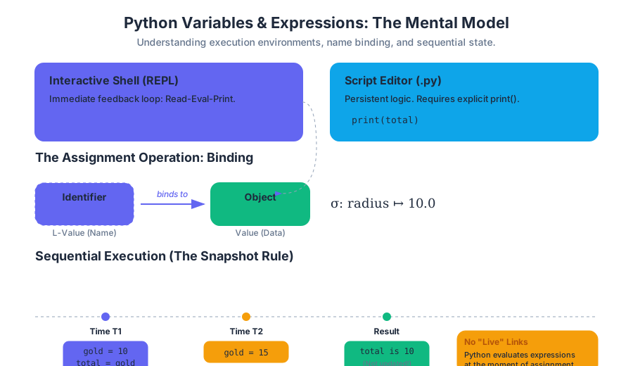
A Python developer operates within two primary contexts: the Interactive Shell (often called the REPL: Read-Eval-Print Loop) and the Script Editor. Understanding the distinction between these is critical for debugging and experimentation.
The Interactive Shell (REPL)
The Shell is a conversational interface. When you type an expression, the interpreter immediately reads it, evaluates it, and prints the result. It is the laboratory of the Python programmer—a place to test small snippets of code, inspect object attributes, or perform quick calculations.
The Script Editor
In contrast, the Editor is used to compose "permanent" programs. Code written here is saved to a .py file and executed in its entirety. Unlike the Shell, the Editor does not automatically print the result of every expression. To see an output from a script, the programmer must explicitly invoke the print() function.
| Feature | Interactive Shell (REPL) | Script Editor (.py file) |
|---|---|---|
| Primary Use | Experimentation, debugging, quick math | Building applications, automation, reusable logic |
| Feedback Loop | Immediate (per line) | Delayed (per execution) |
| Persistence | Lost when the session ends | Saved to disk |
| Output Behavior | Implicitly prints expression results | Requires explicit print() calls |
| Typical Prompt | >>> |
None (Standard text editor) |
Implementation Example: The REPL Interaction
The following block demonstrates a low-level interaction with the Python interpreter, showing how the type and id of objects are inspected in real-time.
# Interacting with the CPython interpreter directly
import sys

# Define a value
x = 42

# Inspecting the object in the shell environment
print(f"Value: {x}")
print(f"Type: {type(x)}")
print(f"Memory Address: {id(x)}")

# Checking the reference count (low-level CPython detail)
# Note: sys.getrefcount(x) will be higher than expected because
# the function itself creates a temporary reference.
print(f"Reference Count: {sys.getrefcount(x)}")
The Mechanics of Variable Assignment
In Python, the statement x = 5 is not a mathematical equation asserting that $x$ is equal to $5$. Instead, it is an assignment operation. Specifically, it is an instruction to the interpreter to bind the identifier (name) on the left to the object (value) on the right.
Syntax Rules for Identifiers
Python enforces strict rules on what constitutes a valid variable name. An identifier must start with a letter or an underscore (_) and can be followed by letters, underscores, or digits. It is case-sensitive (Total and total are distinct).
The L-Value Rule: In an assignment statement, the left-hand side (L-value) must be a valid, single identifier. It cannot be a literal or a complex expression.
| Statement | Validity | Reason |
|---|---|---|
pi = 3.14159 |
Valid | Simple identifier assignment. |
radius_2 = 10 |
Valid | Alphanumeric identifier. |
2_radius = 10 |
Invalid | Identifiers cannot start with a digit. |
x + y = 10 |
Invalid | The L-value must be a name, not an expression. |
5 = x |
Invalid | A literal (5) cannot be assigned a new value. |
Mathematical Derivation of Assignment
We can represent the state of a program as a mapping $\sigma$ from a set of identifiers $I$ to a set of values $V$.
$$ \sigma: I \to V $$
When an assignment $i = e$ is executed, where $i \in I$ and $e$ is an expression that evaluates to $v \in V$, the mapping is updated:
$$ \sigma' = \sigma[i \mapsto v] $$
This means that only the identifier $i$ is updated in the environment. Any other identifier $j$ that was previously defined using $i$ remains mapped to its original value unless explicitly recalculated.
# Pseudocode representation of the Assignment Logic
PROCEDURE Assign(identifier, expression):
    value = EVALUATE(expression)
    IF IS_VALID_IDENTIFIER(identifier):
        ENVIRONMENT.BIND(identifier, value)
    ELSE:
        RAISE SyntaxError("Invalid L-value")
END PROCEDURE
Variable Bindings and Sequential Execution
One of the most common pitfalls for beginners is the "Spreadsheet Misconception." In a spreadsheet, if cell C1 depends on A1, changing A1 automatically updates C1. Python does not work this way.
Python executes code sequentially. When a variable is assigned, it captures the value of the expression at that specific moment in time. If the components of that expression change later, the bound variable remains unchanged.
Worked Example: The Olympic Medal Tally
Consider a script tracking medal counts. If we calculate a total and then update one of the individual counts, the total does not "react" to the change.
# Executing a Python script from the CLI to observe sequential behavior
# Save this as 'medals.py' and run: python3 medals.py

cat << 'EOF' > medals.py
gold = 10
silver = 5
bronze = 8

# Calculate total at Time T1
total = gold + silver + bronze
print(f"Total at T1: {total}") # Output: 23

# Update gold count at Time T2
gold = 15
print(f"Gold updated to: {gold}")

# The 'total' variable is still bound to the result of the T1 calculation
print(f"Total at T2 (without recalculation): {total}") # Output: 23

# To update 'total', we must re-execute the assignment
total = gold + silver + bronze
print(f"Total at T3 (after recalculation): {total}") # Output: 28
EOF

python3 medals.py
The Memory Model: Names vs. Objects
In languages like C++, a variable is often viewed as a "box" in memory where a value is stored. In Python, it is more accurate to think of variables as tags or labels attached to objects.
- Object Creation: The interpreter creates an object (e.g., the integer
23) in memory. - Binding: The name
totalis pointed to that object. - Reassignment: If we say
total = 28, we don't change the number23into28. Instead, we create a new object28and move thetotaltag to it.
Floating-Point Arithmetic and Numerical Representation
Python handles two primary types of numbers: Integers (int), which have arbitrary precision, and Floating-point numbers (float), which represent real numbers using the IEEE 754 standard.
The Precision Problem
Because computers use binary (base 2) to represent numbers, they cannot perfectly represent certain decimal (base 10) fractions. For example, the fraction $1/10$ (0.1) results in a repeating binary sequence, much like $1/3$ results in $0.333...$ in decimal.
This leads to subtle rounding errors that can compromise equality checks.
Theorem of Floating Point Inexactness: For any finite binary representation, there exists a set of decimal fractions that cannot be represented exactly, leading to a representational error $\epsilon$.
| Expression | Expected Result | Actual Python Result |
|---|---|---|
0.1 + 0.2 |
0.3 |
0.30000000000000004 |
0.1 + 0.1 + 0.1 == 0.3 |
True |
False |
2.0 ** 3 |
8.0 |
8.0 |
1 / 3 |
0.333... |
0.3333333333333333 |
Low-Level Representation (C Perspective)
To understand why 0.1 is problematic, we can look at how a double-precision float is structured in memory according to the IEEE 754 standard.
// C code to inspect the binary representation of a float
#include <stdio.h>

void print_binary(unsigned long long n) {
    for (int i = 63; i >= 0; i--) {
        printf("%llu", (n >> i) & 1);
        if (i == 63 || i == 52) printf(" "); // Separate sign, exponent, mantissa
    }
    printf("\n");
}

int main() {
    double val = 0.1;
    unsigned long long *ptr = (unsigned long long *)&val;

    printf("Value: %f\n", val);
    printf("Binary (Sign | Exponent | Mantissa):\n");
    print_binary(*ptr);

    return 0;
}
Best Practices for Arithmetic
- Avoid Equality on Floats: Never use
==with floats. Instead, check if the difference is within a small tolerance (epsilon):abs(x - y) < 1e-9. - Use the
decimalModule: For financial applications where precision is paramount, Python provides thedecimallibrary to avoid binary rounding issues. - Integer Division: Use
//for floor division and%for the modulo (remainder) operator.
Expressions and Operator Precedence
An expression is a combination of values, variables, and operators that the Python interpreter evaluates to produce a single value. The order in which these operations are performed is governed by operator precedence.
Precedence Hierarchy
Python follows standard algebraic rules (PEMDAS/BODMAS), but includes additional operators for programming.
| Precedence | Operator | Description |
|---|---|---|
| 1 (Highest) | ** |
Exponentiation |
| 2 | *, /, //, % |
Multiplication, Division, Floor Div, Modulo |
| 3 | +, - |
Addition, Subtraction |
| 4 | ==, !=, >, < |
Comparisons |
| 5 (Lowest) | and, or, not |
Logical Operators |
Complex Expression Evaluation
Consider the expression: result = 10 + 5 * 2 ** 3.
- Exponentiation:
2 ** 3= 8. - Multiplication:
5 * 8= 40. - Addition:
10 + 40= 50. The variableresultis bound to the object50.
Common Pitfalls and Misconceptions
1. The "Identifier vs. String" Confusion
New programmers often confuse variable names with string literals.
x = 5:xis a name pointing to the value 5.x = "y":xis a name pointing to the string "y".x = y:xis a name pointing to whateveryis currently pointing to. Ifyis undefined, this raises aNameError.
2. Case Sensitivity
temp = 32 and Temp = 32 are two different entries in the interpreter's symbol table. Accessing temp when you defined Temp will result in a failure.
3. Overwriting Built-ins
Python allows you to use built-in function names as variable names (e.g., print = 5). While syntactically valid, this "shadows" the built-in function, making it inaccessible for the remainder of the script.
Pro-Tip: Always avoid using names like
list,str,int, or
Control Flow: Branching and Boolean Logic
Key concepts: Boolean Logic · Comparison Operators · Branching (if-elif-else) · AND operator
Introduces decision-making in programs using conditional statements and logic gates.
Control Flow: Branching and Boolean Logic
In the foundational stages of computational thinking, we treat a program as a recipe: a linear sequence of instructions executed one after another. However, real-world problems are rarely linear. A self-driving car must decide whether to brake or accelerate based on sensor data; a banking script must decide whether to approve a transaction based on a balance check. This capacity for decision-making is known as Control Flow, specifically achieved through Branching and Boolean Logic.
Control flow is the mechanism by which an interpreter or CPU determines the order in which individual statements, instructions, or function calls are executed. Without branching, a program is merely a calculator; with branching, it becomes an agent capable of responding to its environment.
Boolean Logic: The Calculus of Truth
At the heart of every decision in computing lies Boolean Logic, a branch of mathematics centered around two values: True and False (often represented as 1 and 0). Named after George Boole, this algebraic structure allows us to combine simple truth statements into complex logical predicates.
The Boolean Data Type
In Python and most high-level languages, bool is a distinct primitive type. Unlike integers or strings, a boolean variable can only occupy one of two states. This binary nature is the bridge between high-level human reasoning and the low-level "on/off" states of transistors in a processor.
Logical Operators
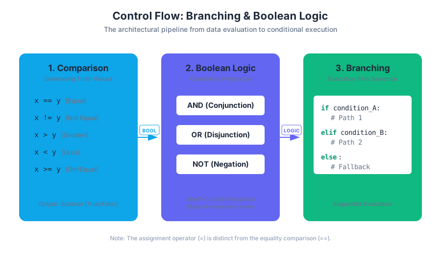
To build complex conditions, we use logical operators. The most fundamental are AND, OR, and NOT.
| Operator | Mathematical Symbol | Description | Requirement for True |
|---|---|---|---|
and |
$\land$ | Conjunction | Both operands must be True. |
or |
$\lor$ | Disjunction | At least one operand must be True. |
not |
$\neg$ | Negation | Flips the truth value (True becomes False). |
The Principle of Bivalence: In standard Boolean logic, every proposition is either true or false. There is no middle ground. This is known as the Law of Excluded Middle.
Comparison Operators: Generating Truth
How do we arrive at a Boolean value? We typically use Comparison Operators to evaluate the relationship between two pieces of data. These operators take two inputs (of various types) and return a single Boolean result.
| Operator | Meaning | Example | Result (if $x=5, y=10$) |
|---|---|---|---|
== |
Equal to | x == y |
False |
!= |
Not equal to | x != y |
True |
> |
Greater than | x > y |
False |
< |
Less than | x < y |
True |
>= |
Greater than or equal to | x >= 5 |
True |
<= |
Less than or equal to | y <= 10 |
True |
Pitfall: Assignment vs. Equality
A common error for beginners is confusing the assignment operator (=) with the equality comparison operator (==).
x = 5tells the computer: "Store the value 5 in the memory location labeled x."x == 5asks the computer: "Is the value currently in x equal to 5?"
Branching: The if-elif-else Construct
Branching is the process of diverting the execution path based on the evaluation of a Boolean expression. In Python, this is implemented using the if, elif, and else keywords.
The if Statement
The if statement is the most basic form of branching. It evaluates a condition; if that condition is True, the indented block of code beneath it executes. If False, the block is skipped.
The elif and else Ladder
Often, we have multiple mutually exclusive conditions. The elif (else if) allows us to check subsequent conditions only if the previous ones failed. The else block serves as a "catch-all" for any case not explicitly handled by the preceding conditions.
Sequential Evaluation
It is critical to understand that Python evaluates these branches sequentially. Once a single condition evaluates to True, its block is executed, and the entire rest of the structure is skipped.
# First code block: Low-level implementation of a multi-branch logic system
# Domain: System Resource Management

def evaluate_system_health(cpu_load, mem_usage, disk_space):
    """
    Determines system status based on hardware metrics.
    Demonstrates nested logic and boolean conjunctions.
    """
    status = "UNKNOWN"

    # Critical failure check (Highest Priority)
    if cpu_load > 95.0 and mem_usage > 95.0:
        status = "CRITICAL_OVERLOAD"
    # Warning states
    elif cpu_load > 80.0 or mem_usage > 80.0:
        if disk_space < 10.0:
            status = "WARNING_LOW_RESOURCES"
        else:
            status = "WARNING_HIGH_LOAD"
    # Healthy state
    elif cpu_load < 50.0 and mem_usage < 50.0 and disk_space > 50.0:
        status = "OPTIMAL"
    # Default fallback
    else:
        status = "STABLE"

    return status

# Example Execution
current_status = evaluate_system_health(85.2, 40.0, 5.0)
print(f"System Health Report: {current_status}")
The AND Operator and Short-Circuit Evaluation
The and operator is a binary operator that returns True only if both inputs are True. However, modern interpreters use a performance optimization called Short-Circuit Evaluation.
Mechanics of Short-Circuiting
When evaluating A and B:
- The interpreter evaluates
A. - If
AisFalse, the entire expressionA and Bmust beFalse, regardless of the value ofB. - Therefore, the interpreter skips the evaluation of
Bentirely.
This is not just a performance trick; it is a vital safety mechanism. It allows us to guard against errors. For example, if (x != 0) and (total / x > 5): will never cause a "Division by Zero" error because if x is 0, the second half of the expression is never touched.
Truth Table for Conjunction (AND)
| Operand A | Operand B | A and B |
|---|---|---|
True |
True |
True |
True |
False |
False |
False |
True |
False |
False |
False |
False |
Comparison with Low-Level Branching
To truly appreciate the elegance of high-level branching, we must look at how the hardware handles these decisions. At the CPU level, there are no if or else keywords. Instead, the processor uses Comparison Instructions and Jump Instructions.
# Second code block: Representation of Branching in Assembly (x86-64)
# This shows how an 'if (x == 5)' block is actually handled by the CPU.

CMP EAX, 5      ; Compare the value in register EAX with the literal 5
JNE .else_label ; Jump to 'else_label' if Not Equal (Zero Flag is not set)

; --- IF BLOCK ---
MOV EBX, 1      ; If equal, set EBX to 1
JMP .end_label  ; Skip the else block

.else_label:
; --- ELSE BLOCK ---
MOV EBX, 0      ; If not equal, set EBX to 0

.end_label:
; Execution continues here...
In this low-level view, "branching" is literal: the Program Counter (the pointer to the next instruction) is forcibly changed to a different memory address based on the result of a comparison.
Real-World Application: Input Validation and the "Lost Forest"
Consider a classic programming exercise: a text-based adventure where a user is "Lost in a Forest." The program must continue running until the user provides the correct input to escape. This combines branching with iteration (loops), but the core logic relies on string comparison.
Case Sensitivity and Logic
When comparing strings, if user_input == "left": is different from if user_input == "Left":. To create a robust program, we use logical or or string normalization.
# Third code block: Real-world usage - Shell Script for Deployment Validation
# Demonstrates branching in a DevOps context (Bash)

#!/bin/bash

DEPLOY_ENV=$1
DISK_USAGE=$(df -h / | grep / | awk '{ print $5 }' | sed 's/%//')

echo "Checking deployment criteria for: $DEPLOY_ENV"

if [ "$DEPLOY_ENV" == "production" ]; then
    if [ "$DISK_USAGE" -gt 90 ]; then
        echo "ERROR: Disk usage too high for production ($DISK_USAGE%)"
        exit 1
    else
        echo "Deployment proceeding to production..."
    fi
elif [ "$DEPLOY_ENV" == "staging" ] || [ "$DEPLOY_ENV" == "dev" ]; then
    echo "Deployment proceeding to non-production environment..."
else
    echo "Usage: $0 {production|staging|dev}"
    exit 1
fi
Advanced Concepts: Nesting and Readability
While branching allows for complex logic, it can lead to the "Arrow Anti-pattern" (or "Nested If Hell"), where code becomes deeply indented and difficult to read.
The Guard Clause Pattern
Instead of nesting logic deep within if statements, senior engineers often use Guard Clauses. This involves checking for invalid conditions early and exiting the function or loop immediately, keeping the "happy path" of the code at the lowest indentation level.
Before (Nested):
if user.is_authenticated:
    if user.has_permission:
        if data.is_valid:
            save_data(data)
        else:
            return "Invalid Data"
    else:
        return "No Permission"
else:
    return "Not Logged In"
After (Guard Clauses):
if not user.is_authenticated:
    return "Not Logged In"
if not user.has_permission:
    return "No Permission"
if not data.is_valid:
    return "Invalid Data"

save_data(data) # Happy path is clean
Common Pitfalls and Edge Cases
- Floating Point Comparison: Never use
==with floating-point numbers (e.g.,0.1 + 0.2 == 0.3isFalsein most languages due to precision errors). Instead, check if the difference is less than a small epsilon:abs(a - b) < 1e-9. - The "Dangling Else": In languages like C++, an
elsealways associates with the closest precedingif. Python avoids this entirely through mandatory indentation, making the structure visually and syntactically unambiguous. - Boolean Coercion (Truthiness): In Python, non-boolean types can be evaluated in an
ifstatement. Integers (except 0), non-empty strings, and non-empty lists are considered "Truthful" (True), while0,None, and empty containers are "Falsy" (False).
Summary of Branching Logic
Branching is the fundamental tool for handling divergent requirements. By combining comparison operators with logical conjunctions (and, or), we can map complex real-world decision matrices into executable code. Whether it is a simple if check or a complex if-elif-else ladder, the goal remains the same: to make the program responsive to the data it processes.
- Boolean: A data type with two possible values:
TrueorFalse. - Comparison Operator: Symbols like
==,>, and!=used to compare values and return a Boolean. - Branching: The process of choosing which code path to follow based on a condition.
- Short-Circuiting: An optimization where the second part of a logical
and/oris skipped if the result is already determined. - Indentation: In Python, the whitespace that defines the scope of a branch.
- Truthiness: The evaluation of non-Boolean objects (like lists or strings) in a Boolean context.
- What is the result of
(5 > 3) and (10 < 5)? - Why is
x = 5different fromx == 5? - In an
if-elif-elsestructure, what happens if both theifand theelifconditions areTrue? - Explain how short-circuit evaluation prevents a "Division by Zero" error.
- What is "truthiness" in the context of an empty Python list
[]? - How does a CPU implement branching without using the
ifkeyword?
Control Flow Mastery Checklist
- Understand Truth Tables: Be able to manually evaluate complex expressions like
not (A or B) and C. - Master Indentation: Recognize that in Python, indentation is the logic. A misplaced space changes the program's meaning.
- Sequential Logic: Remember that the first
Truecondition in anif-elifchain wins. Order your conditions from most specific to most general. - Comparison Precision: Always be wary of comparing floats for equality.
- Guard Clauses: Practice refactoring deeply nested
ifstatements into flat guard clauses for better readability. - Boolean Identity: Understand the difference between
==(value equality) andis(object identity/memory address).
Control Flow: Iteration and Loops
Key concepts: while loops · for loops · range() · break statement
Explains how to repeat tasks efficiently using loops and how to control loop termination.
Control Flow: Iteration and Loops
In the realm of computation, the ability to execute a sequence of instructions once is trivial. The true power of a computer lies in its capacity to perform repetitive tasks with absolute precision and at immense speeds. This concept, known as iteration, allows us to move beyond simple linear scripts and into the domain of complex algorithms.
Iteration is the process of repeatedly executing a block of code, typically until a specific condition is met or a collection of data is exhausted. Without iteration, processing a million-record database would require a million lines of code; with iteration, it requires only a few.
The Philosophy of Iteration: Definite vs. Indefinite
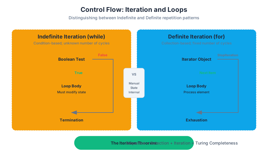
Before diving into syntax, we must distinguish between the two fundamental patterns of repetition:
- Indefinite Iteration: The number of repetitions is not known beforehand. The loop continues as long as a certain logical condition remains true. This is modeled by the
whileloop. - Definite Iteration: The number of repetitions is determined at the start of the loop, usually based on the size of a data structure or a specific range of integers. This is modeled by the
forloop.
The Iteration Theorem: Any computable function can be implemented using only three control structures: sequence, selection (if-statements), and iteration (loops). This underscores that loops are not just a convenience, but a mathematical necessity for general-purpose computing.
While Loops: The Mechanics of Indefinite Iteration
A while loop evaluates a boolean expression before each pass through the loop body. If the expression evaluates to True, the code block is executed. If it evaluates to False, the program skips the block and continues with the next statement in the sequence.
Syntax and Logic Flow
The logic of a while loop is inherently risky. Because the termination depends on a condition that must be modified inside the loop, it is the primary source of "infinite loops"—programs that never terminate because the exit condition is never reached.
| Component | Role | Requirement |
|---|---|---|
| Initialization | Setting the starting state | Must happen before the loop starts |
| Condition | The boolean test | Evaluated at the start of every iteration |
| Loop Body | The work being done | Must eventually affect the Condition |
| Termination | The transition to False |
Essential to prevent system hangs |
Low-Level Implementation
In lower-level languages like C, the while loop is a direct abstraction of a "jump" instruction in assembly.
#include <stdio.h>

/**
 * A robust implementation of a countdown timer.
 * Demonstrates manual state management and boundary conditions.
 */
int main() {
    int counter = 10; // Initialization

    // The condition is checked at the start of each cycle
    while (counter > 0) {
        printf("T-minus %d seconds...\n", counter);

        // Critical: The state must change to ensure eventual termination
        counter--;
    }

    printf("Liftoff!\n");
    return 0;
}
The "Lost Forest" Problem: A Case Study in Indefinite Iteration
A classic pedagogical example involves a user trapped in a "Lost Forest." The program must repeatedly ask the user which direction they want to move. The loop only terminates when the user chooses the correct path. This perfectly illustrates indefinite iteration because the programmer cannot know if the user will take one try or one thousand tries to escape.
Mathematical Representation of Loop Invariants
To prove a loop is correct, computer scientists use a Loop Invariant: a property that is true before and after each iteration.
\text{Let } S \text{ be the set of all possible user inputs.} \\
\text{Let } f(s) \text{ be a function where } f(s) = 1 \text{ if } s \text{ is the exit, else } 0. \\
\text{The loop continues while } \sum_{i=1}^{n} f(s_i) = 0. \\
\text{Termination occurs when } \exists s_n \text{ such that } f(s_n) = 1.
For Loops: Iterating Over Sequences
The for loop in modern languages like Python is more sophisticated than the traditional "counter" loops found in older languages. It is an implementation of the Iterator Pattern, designed to traverse elements in a sequence (strings, lists, tuples, or ranges) automatically.
The Iterator Protocol
When you write for element in sequence:, the interpreter performs the following steps:
- Calls
iter(sequence)to get an iterator object. - Repeatedly calls
next()on that iterator to get the next item. - Catches the
StopIterationexception to terminate the loop gracefully when no items remain.
| Feature | while Loop |
for Loop |
|---|---|---|
| Primary Use | When the end condition is dynamic | When the collection size is known |
| Complexity | Higher risk of infinite loops | Generally safer and more readable |
| State | Manual management (e.g., i += 1) |
Internalized management |
| Performance | Slightly faster in low-level byte manipulation | Optimized for object traversal |
The range() Function: Efficient Definite Iteration
In Python, for loops are frequently paired with the range() function. It is important to understand that range() does not create a list of numbers in memory. Instead, it is a lazy generator (or more accurately, an immutable sequence type) that yields numbers one at a time, making it extremely memory-efficient.
Range Parameters: range(start, stop, step)
- start: The starting integer (inclusive). Defaults to 0.
- stop: The integer at which to stop (exclusive). The loop ends before reaching this number.
- step: The increment between each number. Can be negative for counting downwards.
# Real-world usage: Calculating a weighted moving average
# Demonstrates range() with custom steps and slicing logic

data_points = [10.5, 12.2, 11.8, 13.5, 14.2, 15.1, 14.8]
window_size = 3

print(f"Processing {len(data_points)} samples...")

# Iterate through the list using indices provided by range
for i in range(len(data_points) - window_size + 1):
    window = data_points[i : i + window_size]
    average = sum(window) / window_size
    print(f"Window {i}: {window} -> Avg: {average:.2f}")
Control Flow Alteration: The Break Statement
Sometimes, we need to exit a loop prematurely—before the condition becomes false or the sequence is exhausted. The break statement provides this "emergency exit."
Why use break?
- Efficiency: If you are searching for an item in a list of a billion elements and find it at index 10, there is no need to check the remaining 999,999,990 elements.
- Input Validation: Often used in "infinite" loops (
while True) where the exit condition is complex and checked in the middle of the loop body rather than the start.
The "Search and Destroy" Pattern
Consider a system monitoring a server log for a specific error code. Once found, the system should stop scanning and trigger an alert.
# A conceptual shell-style representation of a loop with a break condition
# Searching for a 'CRITICAL' error in a log file

log_file="server.log"

while read -r line; do
    echo "Checking: $line"
    if [[ "$line" == *"CRITICAL"* ]]; then
        echo "CRITICAL ERROR FOUND. Terminating scan."
        break  # Exits the 'while' loop immediately
    fi
done < "$log_file"

echo "Scan complete or aborted."
Common Pitfalls and Edge Cases
Even senior engineers encounter bugs in loop logic. Understanding these common failure modes is essential for writing robust code.
1. The Off-By-One Error
This occurs when a loop iterates one time too many or one time too few. This is usually caused by a misunderstanding of whether the stop value in a range() or a comparison operator (like < vs <=) is inclusive.
2. Modifying a Collection While Iterating
Never add or remove items from a list while you are looping over it. This shifts the indices and causes the loop to skip elements or crash.
- Solution: Iterate over a copy of the list or use a list comprehension to create a new, filtered list.
3. The Infinite While Loop
If the variables involved in a while condition are never updated inside the loop, the program will hang.
- Debugging Tip: Always include a "safety counter" or print statements during development to track the state of the loop variables.
| Pitfall | Symptom | Prevention |
|---|---|---|
| Infinite Loop | Program stops responding, CPU spikes | Ensure condition variables change |
| Off-By-One | Last item missing or IndexError |
Remember range(n) goes 0 to n-1 |
| Mutation Error | Items skipped during iteration | Iterate over list(my_list[:]) (a copy) |
| Shadowing | Iterator variable overwrites data | Use unique names (e.g., for idx in...) |
Advanced Concept: Nested Loops and Complexity
Loops can be placed inside other loops. This is common when dealing with multi-dimensional data, such as matrices, images (pixels in rows and columns), or coordinate systems.
However, nesting loops significantly impacts Computational Complexity.
- A single loop over $n$ elements is $O(n)$ (Linear time).
- A nested loop (a loop inside a loop) over $n$ elements is $O(n^2)$ (Quadratic time).
If $n = 1,000,000$, an $O(n)$ algorithm takes a million operations, while an $O(n^2)$ algorithm takes a trillion operations. This is the difference between a program that finishes in milliseconds and one that takes hours.
Summary of Best Practices
- Prefer
foroverwhile: If you can define the bounds of your iteration, use aforloop. It is more idiomatic and less prone to errors. - Keep Loop Bodies Small: If a loop body is more than 10–15 lines, consider moving the logic into a separate function. This improves readability and testability.
- Use
breakSparingly: While powerful,breakcan make code harder to follow because it creates multiple exit points. Use it when it clearly simplifies the logic. - Leverage
enumerate(): When you need both the item and its index in aforloop, usefor i, val in enumerate(sequence):instead of manual counters.
Further Reading
- The Art of Computer Programming by Donald Knuth (Volume 1: Fundamental Algorithms)
- Structure and Interpretation of Computer Programs (SICP) - Section on Iterative vs. Recursive processes.
- Python Documentation: "The Iterator Protocol" and "Itertools Module."
String Manipulation and Slicing
Key concepts: String Indexing · String Slicing · Concatenation · Negative Stepping
Focuses on techniques for accessing and modifying text data in Python.
String Manipulation and Slicing
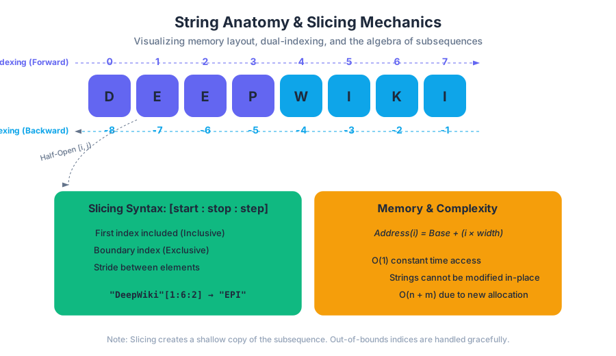
In the hierarchy of computational data types, the string occupies a unique position. While mathematically a string is simply a finite sequence of symbols chosen from an alphabet, in practical computer science, it represents the primary interface between human-readable information and machine-executable logic. Understanding string manipulation is not merely about learning syntax; it is about mastering the mechanics of memory buffers, sequence algebra, and the efficiency of data retrieval.
At its core, a string in modern high-level languages like Python is an immutable sequence object. This immutability is a critical design choice, ensuring that strings can be used as keys in hash maps (dictionaries) and shared across different parts of a program without the risk of side effects. However, this architectural decision necessitates a deep understanding of how to "manipulate" what cannot be changed—leading us to the sophisticated world of indexing, slicing, and concatenation.
String Indexing: The Mechanics of Position
Indexing is the process of accessing a specific element within a sequence based on its ordinal position. In Python, and most modern systems languages, strings use zero-based indexing. This convention is not arbitrary; it stems from the way memory addresses are calculated at the hardware level.
The Zero-Indexing Theorem: If a string starts at memory address $B$ and each character occupies $w$ bytes, the address of the $i$-th character is given by the formula: $Address(i) = B + (i \times w)$ By starting $i$ at 0, the first element resides exactly at the base address $B$, eliminating the need for a subtraction operation during every pointer calculation.
Positive vs. Negative Indexing
Python extends the traditional indexing model by introducing negative indexing, which allows for relative positioning from the end of the sequence. This is particularly useful for accessing trailing data without explicitly calculating the string's length.
| Index Type | Direction | Range (Length $n$) | Use Case |
|---|---|---|---|
| Positive | Forward (Left-to-Right) | $0$ to $n-1$ | Standard iteration, fixed-format parsing. |
| Negative | Backward (Right-to-Left) | $-1$ to $-n$ | Accessing file extensions, suffixes, or last elements. |
Low-Level Implementation of Indexing
To understand why indexing is an $O(1)$ (constant time) operation, we must look at how a string is represented in memory. In a systems-level context, a string is a contiguous block of memory.
/*
 * A low-level representation of a fixed-width character string.
 * This demonstrates how indexing is a direct pointer offset calculation.
 */

#include <stdio.h>

int main() {
    // A string literal stored in the data segment
    const char *str = "DeepWiki";

    // Accessing index 4 ('W')
    // In C, str[4] is syntactic sugar for *(str + 4)
    char element = str[4];

    printf("Base Address: %p\n", (void*)str);
    printf("Address of index 4: %p\n", (void*)(str + 4));
    printf("Value at index 4: %c\n", element);

    return 0;
}
String Slicing: The Algebra of Subsequences
While indexing retrieves a single character, Slicing allows a programmer to extract a contiguous or patterned subsequence. The syntax string[start:stop:step] defines a half-open interval $[start, stop)$, meaning the element at the start index is included, but the element at the stop index is not.
The Anatomy of a Slice
- Start: The index where the slice begins (inclusive). Defaults to 0.
- Stop: The index where the slice ends (exclusive). Defaults to the length of the string.
- Step: The stride between elements. Defaults to 1.
The mathematical beauty of the half-open interval $[i, j)$ is that the length of the resulting slice is simply $j - i$. This avoids the "off-by-one" errors common in languages that use inclusive boundaries.
Slicing Logic and Defaults
The behavior of slicing is governed by a set of internal rules that handle out-of-bounds indices gracefully, unlike standard indexing which raises an IndexError.
| Parameter | Default (Positive Step) | Default (Negative Step) | Behavior if Out of Bounds |
|---|---|---|---|
start |
0 |
len(s) - 1 |
Clamped to string boundaries. |
stop |
len(s) |
-len(s) - 1 |
Clamped to string boundaries. |
step |
1 |
-1 |
Cannot be 0 (raises ValueError). |
Formal Derivation of Slicing
In pseudocode, the slicing operation for s[i:j:k] can be visualized as a loop that constructs a new string object:
Algorithm: StringSlicing(S, start, stop, step)
    Input: String S, Integers start, stop, step
    Output: A new String R

    1. If step > 0:
        lower = max(0, start)
        upper = min(length(S), stop)
    2. Else if step < 0:
        lower = min(length(S) - 1, start)
        upper = max(-1, stop)
    3. Initialize R as empty string
    4. Current = lower
    5. While (step > 0 and Current < upper) or (step < 0 and Current > upper):
        Append S[Current] to R
        Current = Current + step
    6. Return R
Concatenation: Building Sequences
Concatenation is the algebraic operation of joining two character strings end-to-end. In Python, this is achieved via the + operator or the += augmented assignment.
The Performance Trap: Immutability and Memory
Because strings are immutable, every time you concatenate two strings, the runtime must:
- Calculate the total length of the new string.
- Allocate a new block of memory.
- Copy the characters from the first string into the new block.
- Copy the characters from the second string into the new block.
This leads to a classic algorithmic pitfall known as Schlemiel the Painter's algorithm. If you concatenate strings in a loop (e.g., s = s + char), the complexity becomes $O(n^2)$, where $n$ is the final length of the string.
Pro Tip: For large-scale string building, always use the
.join()method or aio.StringIObuffer. The.join()method pre-calculates the required memory and performs the copy in a single pass, maintaining $O(n)$ efficiency.
Real-World Usage: Log Parsing and Path Construction
In professional environments, string manipulation is rarely about simple "Hello World" examples. It is used for parsing structured data from raw streams.
import os

def process_log_entry(raw_line):
    """
    Example of slicing and concatenation in a production context.
    Extracts a timestamp and appends a status code.
    """
    # Assume log format: "2023-10-27 10:00:00 [INFO] User logged in"
    # Extracting the ISO timestamp (first 19 characters)
    timestamp = raw_line[:19]

    # Extracting the log level using slicing
    # We look for the index of '[' and ']'
    start_idx = raw_line.find("[") + 1
    end_idx = raw_line.find("]")
    log_level = raw_line[start_idx:end_idx]

    # Concatenation to form a structured record
    # Using f-strings (modern concatenation) for readability and speed
    return f"{timestamp} | STATUS: {log_level}"

# Example invocation
log = "2023-10-27 14:30:05 [ERROR] Database connection failed"
print(process_log_entry(log))
Negative Stepping and String Reversal
The step parameter in slicing is a powerful tool for data transformation. When the step is negative, the slicing engine traverses the string from right to left.
The Reversal Idiom
The most common use of negative stepping is the "reversal idiom": s[::-1].
startdefaults to the end of the string.stopdefaults to the beginning (and includes the first character).stepis-1.
Advanced Stepping: Downsampling and Striding
Negative stepping can be combined with specific start and stop values to extract patterns in reverse. For example, s[10:2:-2] would start at index 10 and move toward index 2, taking every second character.
Common Pitfalls and Edge Cases
- IndexError vs. Slicing Grace: Accessing
s[100]on a 10-character string will crash your program. However,s[0:100]will simply return the whole string. This "silent clamping" can sometimes hide logic errors in your code. - Off-by-One in Slicing: Remember that the
stopindex is not included. If you want the first three characters, you uses[0:3], which returns indices 0, 1, and 2. - Memory Overhead: Slicing creates a copy of the data (in Python). If you are slicing a 1GB string in a loop, you will quickly exhaust your system's RAM. In such cases, consider using
memoryvieworbytearrayfor zero-copy operations.
Comparison of String Access Methods
| Method | Syntax | Result Type | Complexity | Out-of-Bounds Behavior |
|---|---|---|---|---|
| Indexing | s[i] |
Single Char | $O(1)$ | Raises IndexError |
| Slicing | s[i:j] |
Substring | $O(k)$* | Returns empty string or partial |
| Stride Slicing | s[i:j:k] |
Patterned Substring | $O(n/k)$ | Returns empty string or partial |
| Concatenation | s1 + s2 |
New String | $O(n+m)$ | N/A |
*where k is the length of the slice.
Practical Application: Data Sanitization
In DevOps and Infrastructure, string manipulation is frequently used to sanitize inputs or transform configuration strings.
#!/bin/bash
# A shell script demonstrating string manipulation for environment variables

RAW_URL="https://user:password@internal-service.cluster.local:8080/api/v1"

# 1. Extracting the Protocol (Slicing via parameter expansion)
# Syntax: ${variable%%suffix}
PROTOCOL="${RAW_URL%%://*}"

# 2. Extracting the Hostname
# Remove everything up to '@' and everything after ':'
TEMP="${RAW_URL#*@}"
HOSTNAME="${TEMP%:*}"

# 3. Concatenation to build a new connection string
NEW_URL="${PROTOCOL}://${HOSTNAME}/health"

echo "Original: $RAW_URL"
echo "Sanitized: $NEW_URL"
Summary of Theoretical Constraints
When we discuss string manipulation, we are essentially discussing the management of linear arrays of bytes. The high-level abstractions provided by Python (like negative stepping) are built upon low-level pointer arithmetic. The efficiency of your code depends on minimizing the number of allocations (avoiding + in loops) and understanding the boundaries of your sequences.
Functions and Decomposition
Key concepts: Function Definitions · Return vs. Print · Scope · Implicit Return (None)
Introduces the concept of breaking programs into reusable, modular components.
Functions and Decomposition
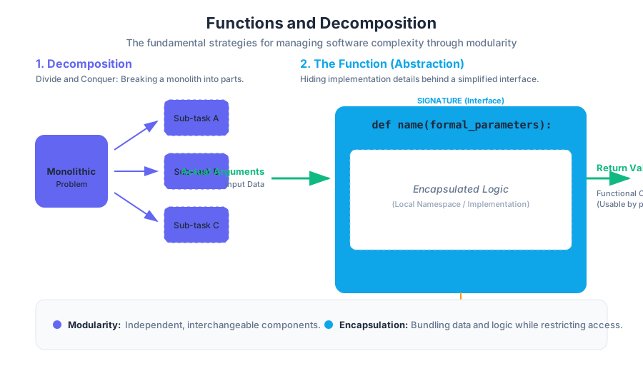
In the realm of software engineering and computational theory, the transition from writing linear scripts to architecting modular systems marks the birth of a professional programmer. As programs grow in complexity, the human mind struggles to maintain a "flat" mental model of thousands of lines of code. To combat this, we employ two fundamental strategies: Decomposition and Abstraction.
Decomposition is the process of breaking a large, monolithic problem into smaller, self-contained sub-problems. Abstraction, conversely, is the practice of hiding the internal details of those sub-problems behind a simplified interface. Together, these concepts are realized through the Function—the primary unit of modularity in almost every modern programming language.
The Philosophy of Modularity: Decomposition and Abstraction
Before diving into syntax, one must understand the "Why." Why not simply write one long list of instructions? The answer lies in the limits of human cognition and the necessity of code reuse.
Decomposition: Divide and Conquer
Decomposition allows a developer to divide a project among multiple team members or simply manage their own cognitive load. By breaking a task like "Build a Search Engine" into "Web Crawler," "Indexer," and "Query Processor," we transform an impossible task into a series of manageable ones.
Abstraction: The Black Box
Abstraction allows us to use a piece of code without needing to understand how it works internally. When you use the math.sqrt() function, you do not need to know if it uses Newton’s method or a lookup table; you only need to know the input (a number) and the output (its square root). This is often referred to as the Black Box model.
| Concept | Goal | Real-World Analogy |
|---|---|---|
| Decomposition | Divide a complex task into smaller parts. | A restaurant kitchen divided into stations (grill, salad, pastry). |
| Abstraction | Hide implementation details; focus on the interface. | A car's steering wheel; you don't need to see the rack and pinion to turn. |
| Modularity | Create interchangeable, independent components. | Lego bricks that can be combined in various ways. |
| Encapsulation | Bundle data and methods while restricting access. | A medicine capsule containing specific ingredients. |
Anatomy of a Function Definition
In Python, a function is a reusable block of code that is executed only when called. The definition of a function establishes its Signature (name and parameters) and its Body (the logic).
Definition: Function A function is a mapping from a set of inputs (domain) to a set of outputs (codomain), encapsulated within a named block that defines a local namespace.
The Syntax of def
The def keyword signals the start of a function definition. This is followed by the function name, a set of parentheses containing formal parameters, and a colon. The indented block that follows is the function's scope.
def calculate_bisection_root(objective_function, low, high, epsilon=1e-7):
    """
    Finds the root of a function within a given interval [low, high]
    using the Bisection Method.

    Parameters:
    objective_function (callable): The function to evaluate.
    low (float): Lower bound of the interval.
    high (float): Upper bound of the interval.
    epsilon (float): Convergence threshold.

    Returns:
    float: The approximate root of the function.
    """
    if objective_function(low) * objective_function(high) >= 0:
        raise ValueError("The function must have different signs at the boundaries.")

    ans = (high + low) / 2.0
    while (high - low) / 2.0 > epsilon:
        if objective_function(ans) == 0:
            return ans
        elif objective_function(low) * objective_function(ans) < 0:
            high = ans
        else:
            low = ans
        ans = (high + low) / 2.0
    return ans
Formal Parameters vs. Actual Arguments
A common point of confusion is the distinction between parameters and arguments.
- Formal Parameters: The variables listed in the function definition (e.g.,
low,highabove). They act as placeholders. - Actual Arguments: The real values passed to the function when it is invoked (e.g.,
calculate_bisection_root(f, 0, 10)).
Mapping Inputs to Outputs
Mathematically, a function $f$ can be represented as:
f: X \to Y
\text{where } X \text{ is the set of inputs (Arguments) and } Y \text{ is the set of outputs (Return Values).}
In a more programmatic pseudocode representation:
ALGORITHM FunctionInvocation(func_name, args):
    1. Create a new local symbol table (Stack Frame).
    2. Bind actual arguments to formal parameters in the local table.
    3. Execute the function body line by line.
    4. If 'return' is encountered, exit and yield the value to the caller.
    5. If the end is reached without 'return', yield 'None'.
    6. Destroy the local symbol table.
Return vs. Print: The Fundamental Distinction
For beginners, the difference between return and print() is often the most significant hurdle. This stems from the fact that both appear to "output" something to the screen during interactive testing. However, their roles in a program's architecture are diametrically opposed.
The print() Function
print() is a side effect. It communicates with the external world (the console) but does not provide data back to the program's internal logic. A value that is printed is "lost" to the program; it cannot be stored in a variable for later calculation.
The return Statement
return is the functional output. It terminates the function's execution and hands a value back to the line of code that called it. This allows for Composition, where the output of one function becomes the input of another.
| Feature | print() |
return |
|---|---|---|
| Purpose | Human-readable output (debugging/logging). | Program-readable output (data flow). |
| Data Flow | Exits the program environment to the console. | Stays within the program environment. |
| Function Execution | Continues after the print statement. | Immediately terminates the function. |
| Variable Assignment | Returns None; cannot be assigned. |
Can be assigned to a variable for future use. |
| Analogy | A chef shouting "Order up!" | A chef handing the plate to the waiter. |
Example: The Cost of Confusion
Consider a scenario where we need to calculate the total cost of an item including tax.
# INCORRECT: Using print instead of return
def calculate_tax_print(price):
    print(price * 0.05)

# CORRECT: Using return
def calculate_tax_return(price):
    return price * 0.05

# Usage
subtotal = 100
tax = calculate_tax_print(subtotal) # tax is now None!
# total = subtotal + tax  <-- This will throw a TypeError: int + NoneType

tax_actual = calculate_tax_return(subtotal) # tax_actual is 5.0
total = subtotal + tax_actual # total is 105.0 (Success)
Implicit Return and the None Type
In Python, every function returns something. If you do not explicitly include a return statement, or if the function reaches the end of its body without hitting a return, Python executes an Implicit Return.
The None Singleton
Noneis a special constant in Python representing the absence of a value. It is the sole instance of theNoneTypeclass.
When a function lacks a return, it implicitly returns None. This is why calling print(print("Hello")) results in:
Hello(from the inner print)None(from the outer print, because the inner print returnedNone)
Scope and the Symbol Table
Scope refers to the region of a program where a particular variable name is "visible" or accessible. Python uses a system of Namespaces (symbol tables) to manage these variables.
The LEGB Rule
Python resolves variable names using the LEGB priority:
- Local: Variables defined inside the current function.
- Enclosing: Variables in the local scope of any enclosing functions (relevant in nested functions).
- Global: Variables defined at the top level of the script or module.
- Built-in: Names pre-defined by Python (e.g.,
len,range,ValueError).
The Stack Frame
When a function is called, the Python interpreter creates a Stack Frame. This is a private block of memory that stores the function's local variables. Once the function returns, this frame is "popped" off the stack and destroyed, meaning local variables cease to exist.
Scope Isolation Example
x = 10 # Global Scope

def outer_function():
    x = 20 # Enclosing Scope (local to outer_function)

    def inner_function():
        x = 30 # Local Scope (local to inner_function)
        print(f"Inner x: {x}")

    inner_function()
    print(f"Outer x: {x}")

outer_function()
print(f"Global x: {x}")
Output:
Inner x: 30
Outer x: 20
Global x: 10
Each x exists in a different symbol table. Modifying the local x inside inner_function has no effect on the x in outer_function or the global x.
Argument Passing Mechanics
Python uses a mechanism often called Pass-by-Object-Reference (or Call-by-Sharing).
- If you pass an immutable object (like an integer, string, or tuple), the function cannot modify the original variable in the caller's scope. It can only rebind the local name to a new object.
- If you pass a mutable object (like a list or dictionary), the function can modify the contents of that object, and those changes will be visible to the caller.
Default Arguments and the "Mutable Default" Trap
One of the most common pitfalls in Python is using a mutable object (like a list) as a default argument.
# DANGEROUS: The list is created once at definition time, not at call time.
def append_to_list(val, my_list=[]):
    my_list.append(val)
    return my_list

print(append_to_list(1)) # [1]
print(append_to_list(2)) # [1, 2] -- Unexpected!

# SAFE: Use None as a placeholder
def append_to_list_safe(val, my_list=None):
    if my_list is None:
        my_list = []
    my_list.append(val)
    return my_list
Practical Application: Decomposition in Action
To illustrate the power of decomposition, let's look at a task: Analyzing a text file for word frequency.
Instead of one giant loop, we decompose it into three distinct functions.
import string

def clean_text(raw_text):
    """Removes punctuation and converts to lowercase."""
    return raw_text.translate(str.maketrans('', '', string.punctuation)).lower()

def count_frequencies(word_list):
    """Creates a dictionary mapping words to their occurrence count."""
    freq_map = {}
    for word in word_list:
        freq_map[word] = freq_map.get(word, 0) + 1
    return freq_map

def get_top_n(freq_map, n=5):
    """Returns the top N most frequent words."""
    return sorted(freq_map.items(), key=lambda item: item[1], reverse=True)[:n]

# The 'Orchestrator' logic
raw_data = "The quick brown fox jumps over the lazy dog. The dog was not amused!"
words = clean_text(raw_data).split()
frequencies = count_frequencies(words)
top_words = get_top_n(frequencies, 3)

print(f"Analysis Complete. Top words: {top_words}")
Real-World Invocation (CLI)
In a professional environment, these functions might be part of a larger utility invoked via the command line.
# Example of how a decomposed script might be used in a pipeline
cat document.txt | python3 word_analyzer.py --top 10 --exclude-stopwords
Summary of Best Practices
- Function Length: A function should ideally do one thing and do it well. If a function is longer than a single screen (20-30 lines), it is likely a candidate for further decomposition.
- Docstrings: Always include a docstring explaining the parameters, return type, and purpose. This is the "User Manual" for your abstraction.
- Pure Functions: Whenever possible, write Pure Functions—functions that have no side effects (like printing or modifying global variables) and always return the same output for the same input. These are much easier to test and debug.
- Avoid Global Variables: Relying on global variables inside functions breaks abstraction, as the function now depends on the state of the entire program rather than just its inputs.
Higher-Order Functions
Key concepts: Functions as Arguments · Parameter Mapping · Execution Flow
Explores advanced function usage where functions act as data.
Higher-Order Functions
In the landscape of computational abstraction, the transition from treating data as passive entities to treating logic as a manipulatable resource marks the threshold of advanced programming. Higher-Order Functions (HOFs) represent this transition. In languages like Python, JavaScript, and Swift, functions are categorized as first-class objects, a designation that elevates them from mere subroutines to entities that can be stored in variables, passed as arguments, and returned from other functions.
At its core, a higher-order function is defined by a simple but profound criterion: it must either take one or more functions as arguments or return a function as its result. This capability allows for the creation of "meta-programs"—code that describes how other code should be executed. By decoupling the iteration logic from the transformation logic, HOFs enable a level of modularity that is impossible with standard procedural flow.
The Foundation: Functions as First-Class Citizens
Before exploring the mechanics of HOFs, we must establish the prerequisite: the First-Class Object. In a programming language, an object is "first-class" if it supports all the operations generally available to other entities. This includes being passed as an argument, returned from a function, and assigned to a variable.
| Property | Description | Impact on Functions |
|---|---|---|
| Assignment | Can be assigned to a variable name or stored in a data structure. | func_ptr = my_function allows aliasing and dynamic selection. |
| Passability | Can be passed as an argument to a procedure. | Enables "Inversion of Control" (IoC) and callbacks. |
| Returnability | Can be the return value of a procedure. | Enables factory patterns and closures. |
| Identity | Has a distinct identity and type (e.g., <class 'function'>). |
Allows for runtime introspection and type checking. |
Definition: Higher-Order Function (HOF) A function $f$ is higher-order if it satisfies the mapping $f: (A \to B) \times C \to D$, where at least one input or the output is itself a function mapping.
Functions as Arguments: Inversion of Control
The most common application of HOFs is passing a function as an argument. This pattern is often referred to as Inversion of Control (IoC). Instead of a function deciding exactly how to process every piece of data, it accepts a "strategy" (in the form of another function) from the caller.
Why It Matters
Consider a scenario where you need to compute the sum of integers in a list. Later, you need the sum of their squares, and then the sum of their absolute values. Without HOFs, you would write three distinct loops. With HOFs, you write one accumulate function that accepts a transform function as a parameter.
Mechanics of Implementation
When a function is passed as an argument, the receiving function does not execute it immediately. Instead, it receives a reference to the function's entry point in memory. The execution happens "later," within the scope of the higher-order function, often repeatedly.
# First code block: Low-level implementation of a generic accumulator
# This demonstrates the primary mechanism of HOFs in Python.

def apply_and_sum(data_list, transform_func):
    """
    A higher-order function that applies transform_func to each
    element in data_list and returns the aggregate sum.
    """
    total = 0
    for item in data_list:
        # The 'transform_func' is invoked here, inside the HOF's scope.
        # This is the 'callback' mechanism.
        total += transform_func(item)
    return total

def square(x):
    return x * x

def cube(x):
    return x ** 3

# Usage
numbers = [1, 2, 3, 4, 5]
sum_of_squares = apply_and_sum(numbers, square)
sum_of_cubes = apply_and_sum(numbers, cube)

print(f"Squares: {sum_of_squares}, Cubes: {sum_of_cubes}")
Parameter Mapping and Binding
A critical aspect of HOFs is Parameter Mapping—the process by which the arguments of the higher-order function are bound to the formal parameters of the passed function. This requires a strict contract between the HOF and the function it receives.
Formal vs. Actual Parameters
When we define apply_and_sum(data_list, transform_func), transform_func is a formal parameter. When we call it with apply_and_sum(my_list, square), square is the actual parameter. The HOF must know the arity (number of arguments) that the transform_func expects. If apply_and_sum passes one argument but transform_func requires two, the program will raise a TypeError.
Trace Table: Execution Flow of apply_and_sum(numbers, square)
Assuming numbers = [1, 2]:
| Step | Scope | Variable | Value/Action |
|---|---|---|---|
| 1 | Global | numbers |
[1, 2] |
| 2 | Global | square |
<function square at 0x...> |
| 3 | apply_and_sum |
data_list |
Reference to numbers |
| 4 | apply_and_sum |
transform_func |
Reference to square |
| 5 | Loop Iter 1 | item |
1 |
| 6 | square |
x |
1 (Bound from item) |
| 7 | Loop Iter 1 | total |
0 + 1 = 1 |
| 8 | Loop Iter 2 | item |
2 |
| 9 | square |
x |
2 (Bound from item) |
| 10 | Loop Iter 2 | total |
1 + 4 = 5 |
Mathematical Derivation: Functional Abstraction
In mathematical terms, HOFs are akin to operators in calculus. Consider the derivative operator $D$. It does not take a number as an input; it takes a function $f(x)$ and returns another function $f'(x)$.
% Second code block: Mathematical representation of HOFs
% Representing the Derivative as a Higher-Order Function

Let F be the set of all differentiable functions.
The derivative operator D is a mapping:
D: F -> F

Where for any f ∈ F:
(D(f))(x) = lim_{h -> 0} [f(x + h) - f(x)] / h

In pseudocode, this HOF 'derivative' would look like:
function derivative(f, dx):
    return function(x):
        return (f(x + dx) - f(x)) / dx
This derivation highlights the "Function as Return Value" aspect of HOFs. The derivative function doesn't return a number; it returns a new function that can be evaluated at any $x$.
Execution Flow and the Call Stack
The execution flow of a higher-order function involves complex movements within the Call Stack. When a HOF calls its argument function, a new Activation Record (or stack frame) is pushed onto the stack.
- HOF Entry: The stack frame for the HOF is created, containing its local variables and the references to the passed functions.
- Callback Invocation: The HOF pauses its execution to call the argument function. A new frame is pushed for the callback.
- Callback Exit: The callback completes, its frame is popped, and the return value is passed back to the HOF.
- HOF Resumption: The HOF uses the returned value to continue its logic.
Visualizing the Stack
Theorem: The Principle of Least Knowledge A higher-order function should not need to know the internal implementation of the function it calls. It only requires that the function adheres to the expected interface (input types and return types). This is the basis for Polymorphism in functional programming.
Real-World Application: Middleware and Event Handling
In modern software engineering, HOFs are the backbone of asynchronous programming and web frameworks. In JavaScript, for example, the addEventListener function is a classic HOF that takes an event type and a callback function.
// Third code block: Real-world usage in Web APIs
// Demonstrating HOFs in an Express.js-style middleware pipeline.

const loggerMiddleware = (req, res, next) => {
    console.log(`${new Date().toISOString()} - ${req.method} ${req.url}`);
    // 'next' is a function passed as an argument.
    // Calling it passes control to the next HOF in the chain.
    next();
};

const authMiddleware = (req, res, next) => {
    if (req.headers.authorization) {
        next();
    } else {
        res.status(401).send('Unauthorized');
    }
};

// A HOF that 'composes' multiple middleware into one
const compose = (fns) => (req, res) => {
    const dispatch = (i) => {
        const fn = fns[i];
        if (!fn) return;
        fn(req, res, () => dispatch(i + 1));
    };
    dispatch(0);
};

// Usage in a hypothetical server
const appPipeline = compose([loggerMiddleware, authMiddleware]);
The Functional Trinity: Map, Filter, and Reduce
Most HOF usage centers around three fundamental patterns. These patterns replace explicit loops with declarative transformations.
| Pattern | Mathematical Analogy | Purpose | Result Type |
|---|---|---|---|
| Map | $f(x) \forall x \in S$ | Transforms every element in a collection. | Collection of same size. |
| Filter | ${x \in S \mid P(x)}$ | Selects elements that satisfy a predicate $P$. | Collection of equal or smaller size. |
| Reduce | $\sum$ or $\prod$ | Aggregates a collection into a single value. | Single value (scalar/object). |
Map: The Transformer
map takes a function and a list, applying the function to every element. It is the purest form of "Parameter Mapping" where the HOF manages the iteration and the callback manages the logic.
Filter: The Gatekeeper
filter takes a predicate (a function that returns a Boolean). It constructs a new list containing only elements for which the predicate returns True.
Reduce: The Folding Operator
reduce (or fold) is the most complex. It takes a binary function, a collection, and an optional initial value. It "folds" the collection by repeatedly applying the function to an accumulator and the next element.
Common Pitfalls and Edge Cases
While HOFs are powerful, they introduce specific categories of bugs that are often difficult to trace.
1. Late Binding and Closures
In many languages (like Python), variables used inside a nested function are looked up when the function is called, not when it is defined. This can lead to unexpected behavior in loops.
2. Side Effects in Callbacks
HOFs assume that the passed function is pure (produces no side effects). If a callback modifies a global variable or performs I/O, the HOF's behavior becomes unpredictable, especially in parallel execution environments.
3. Arity Mismatch
As mentioned in the Parameter Mapping section, passing a function that expects three arguments to a HOF that only provides two will cause a runtime crash.
4. Performance Overhead
Each function call involves stack operations. In performance-critical systems (like embedded C), excessive use of HOFs (via function pointers) can introduce overhead compared to inlined loops.
/* Fourth code block: Low-level C implementation showing function pointers */
/* This illustrates how HOFs are handled at the machine level. */

#include <stdio.h>

// Define a type for a function that takes an int and returns an int
typedef int (*transformer)(int);

// The Higher-Order Function in C
void process_array(int *arr, int size, transformer func) {
    for (int i = 0; i < size; i++) {
        // Dereferencing the function pointer to execute the logic
        arr[i] = (*func)(arr[i]);
    }
}

int increment(int x) { return x + 1; }
int double_val(int x) { return x * 2; }

int main() {
    int data[] = {10, 20, 30};
    // Passing the address of the 'double_val' function
    process_array(data, 3, double_val);

    for(int i=0; i<3; i++) printf("%d ", data[i]); // Output: 20 40 60
    return 0;
}
Summary of Execution Flow
When a Higher-Order Function executes, it creates a dynamic bridge between different layers of abstraction. The "Execution Flow" is not linear; it is a series of jumps:
- Entry: The HOF captures the environment.
- Mapping: The HOF prepares the data for the callback.
- Dispatch: Control is handed to the callback.
- Collection: The HOF retrieves the result and integrates it into the larger computation.
This cycle repeats for every element in the data structure, effectively "outsourcing" the core logic while maintaining control over the process structure.
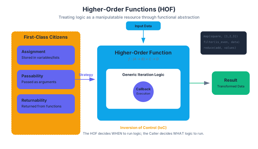
Data Structures: Tuples and Lists
Key concepts: Tuples · List Mutation · Indexing · Trailing Commas
Introduces compound data types for storing collections of information.
Data Structures: Tuples and Lists
In the realm of computation, we have moved from simple scalar types—integers, floats, and booleans—to the concept of compound data structures. While a single variable can hold a single value, a data structure allows us to organize and store collections of data. In Python, the two most fundamental sequential structures are Tuples and Lists.
Understanding these is not merely a matter of syntax; it is a study of memory management, the philosophy of immutability, and the mechanics of aliasing. A senior engineer chooses between a list and a tuple not based on habit, but based on the requirements of data integrity and computational efficiency.
The Nature of Sequences
Both tuples and lists are classified as sequences. A sequence is an ordered collection of objects where each element is associated with an integer index. This ordering is crucial: it allows for deterministic retrieval and predictable iteration.
Definition: Sequence A sequence $S$ is a mapping from a set of indices ${0, 1, \dots, n-1}$ to a set of elements $E$, where $n$ is the length of the sequence. For any index $i$, $S[i]$ returns the element at that position.
| Feature | Tuples | Lists |
|---|---|---|
| Syntax | (element1, element2) |
[element1, element2] |
| Mutability | Immutable (cannot change) | Mutable (can change) |
| Memory Overhead | Lower (fixed size) | Higher (dynamic resizing) |
| Common Use Case | Fixed records, function returns | Collections of similar items, stacks |
| Hashability | Hashable (if elements are hashable) | Unhashable |
Tuples: The Immutable Record
A Tuple is an immutable sequence of Python objects. Once a tuple is created, its length and the identity of its elements cannot be altered. This immutability provides a "contract" of safety: if you pass a tuple to a function, you are guaranteed that the function cannot modify the structure of that data.
The Syntax of Singleton Tuples
A common pitfall for beginners is the definition of a single-element tuple. Because parentheses () are also used for grouping expressions (e.g., (2 + 3) * 5), Python requires a trailing comma to distinguish a tuple from a parenthesized expression.
t = (5)$\rightarrow$ Evaluates to the integer5.t = (5,)$\rightarrow$ Evaluates to a tuple containing the integer5.
Tuple Unpacking and Return Values
Tuples are the engine behind Python's ability to return multiple values from a function. This is technically the return of a single tuple object, which is then "unpacked" by the caller.
# First code block: Low-level implementation and advanced unpacking
def get_coordinate_metrics(points):
    """
    Calculates the bounding box of a set of 2D points.
    Demonstrates tuple creation and nested unpacking.
    """
    if not points:
        return (0, 0, 0, 0)

    # Initialize min/max with first point
    min_x = max_x = points[0][0]
    min_y = max_y = points[0][1]

    for (x, y) in points: # Unpacking in loop header
        if x < min_x: min_x = x
        if x > max_x: max_x = x
        if y < min_y: min_y = y
        if y > max_y: max_y = y

    # Returning a tuple (parentheses are optional but recommended)
    return (min_x, max_x, min_y, max_y)

# Usage
data = [(1.2, 3.4), (0.5, 9.1), (4.5, 2.2)]
x_low, x_high, y_low, y_high = get_coordinate_metrics(data)

print(f"Bounds: X[{x_low}:{x_high}], Y[{y_low}:{y_high}]")
Lists: The Dynamic Array
A List is a mutable sequence. Unlike tuples, lists are designed to grow, shrink, and change. In the underlying CPython implementation, a list is an array of pointers to other objects. When you "mutate" a list, you are changing which pointers are stored in that array, or changing the size of the array itself.
List Mutation and Memory
Because lists are mutable, they require a more complex memory strategy. To avoid reallocating memory every time an element is added (an $O(N)$ operation), Python uses over-allocation. It reserves more space than is currently needed, allowing append operations to occur in amortized $O(1)$ time.
# Second code block: Mathematical derivation of List Growth
# Let C be the capacity of the underlying array and N be the number of elements.
# When N > C, a new array is allocated with capacity C'.

C' = (N >> 3) + (N < 9 ? 3 : 6) + N

# This growth factor (roughly 1.125x) ensures that:
# 1. Memory is not wasted excessively (unlike a 2x doubling strategy).
# 2. The frequency of reallocations decreases as the list grows.
# 3. The cost of copying elements is spread out (amortized) over many appends.
Indexing and Slicing
Both structures support Indexing (accessing a single element) and Slicing (accessing a sub-sequence). Python uses zero-based indexing, which aligns with the mathematical concept of an "offset" from the start of the memory block.
The Slicing Formula
The syntax sequence[start:stop:step] follows a specific logic:
- Start: The index of the first element to include (inclusive).
- Stop: The index to stop at (exclusive).
- Step: The increment between indices.
| Expression | Result | Description |
|---|---|---|
L[0] |
First element | Standard access |
L[-1] |
Last element | Negative indexing (wraps around) |
L[1:4] |
[L[1], L[2], L[3]] |
Basic slice |
L[::-1] |
Reversed sequence | Slice with negative step |
L[:2] |
First two elements | Omitted start defaults to 0 |
L[2:] |
From index 2 to end | Omitted stop defaults to length |
Mutation, Aliasing, and Cloning
This is the most critical concept for any developer to master. When you assign a list to a new variable, you are not creating a copy of the data. You are creating an alias.
The Pointer Problem
Consider the following:
L1 = [1, 2, 3]
L2 = L1
L2.append(4)
print(L1) # Outputs [1, 2, 3, 4]
In this example, L1 and L2 point to the same object in memory. This is known as aliasing. If you want a distinct copy, you must perform cloning.
Cloning Techniques
- Slicing:
L2 = L1[:] - Factory Method:
L2 = list(L1) - Deep Copy: For nested lists,
copy.deepcopy(L1)is required to copy the internal objects as well.
Methods of List Manipulation
Lists come equipped with a suite of methods that modify the list "in-place." These methods typically return None, reinforcing the idea that the object itself has changed rather than a new object being created.
| Method | Complexity | Action |
|---|---|---|
append(x) |
$O(1)$* | Adds x to the end of the list. |
extend(iterable) |
$O(K)$ | Appends all elements from the iterable. |
insert(i, x) |
$O(N)$ | Inserts x at index i, shifting subsequent elements. |
pop(i) |
$O(N)$ | Removes and returns element at i (defaults to last). |
remove(x) |
$O(N)$ | Removes the first occurrence of value x. |
sort() |
$O(N \log N)$ | Sorts the list in-place using Timsort. |
reverse() |
$O(N)$ | Reverses the elements in-place. |
Theorem: The Mutability Trap Never iterate over a list while mutating its length. Because the iterator tracks the current index, removing an element shifts all subsequent elements to the left, causing the iterator to skip the next item.
# Third code block: Real-world usage via CLI and Python one-liners
# Scenario: Filtering a list of system logs and extracting PIDs

cat system.log | python3 -c "
import sys
# Read lines into a list, strip whitespace, and filter for 'ERROR'
logs = [line.strip() for line in sys.stdin if 'ERROR' in line]
# Extract PIDs (assuming format 'ERROR [PID]: message')
pids = [log.split('[')[1].split(']')[0] for log in logs]
# Convert to a tuple for immutable storage/hashing
unique_pids = tuple(set(pids))
print(f'Unique Error PIDs: {unique_pids}')
"
Advanced Concept: Nested Data Structures
Tuples and lists can contain other tuples and lists. This allows for the representation of complex data, such as matrices or trees. However, nesting introduces complexity in mutability.
The "Immutable" Tuple with Mutable Elements
A tuple is immutable in that its bindings cannot change. However, if a tuple contains a list, that list can still be modified.
# Fourth code block: Edge case - Nested Mutability
# A tuple containing a mutable list
entry = ("ID_001", [10, 20, 30])

try:
    # This will fail: Tuples don't support item assignment
    entry[0] = "ID_002"
except TypeError as e:
    print(f"Expected Error: {e}")

# This will SUCCEED: The list inside the tuple is being mutated
entry[1].append(40)
print(f"Modified Entry: {entry}")
# Result: ('ID_001', [10, 20, 30, 40])
Performance Considerations
When choosing between these structures, consider the scale of your data.
- Iteration Speed: Tuples are slightly faster to iterate over than lists.
- Memory Footprint: Tuples are more memory-efficient. A list must store its size, its allocated capacity, and the pointer to the array. A tuple only stores its size and the pointers.
- Safety: Use tuples for fixed configurations, dictionary keys (lists cannot be keys because they are not hashable), and returning multiple values. Use lists for collections that will change during the program's execution.
Summary of Best Practices
- Default to Tuples for data that shouldn't change. It signals intent to other developers and prevents accidental bugs.
- Use List Comprehensions for creating lists. They are more readable and often faster than manual loops with
append. - Be Wary of Aliasing. If you pass a list to a function and that function modifies it, the original list is changed. If this is not desired, pass a clone:
my_function(my_list[:]). - Trailing Commas are mandatory for single-element tuples:
(x,).
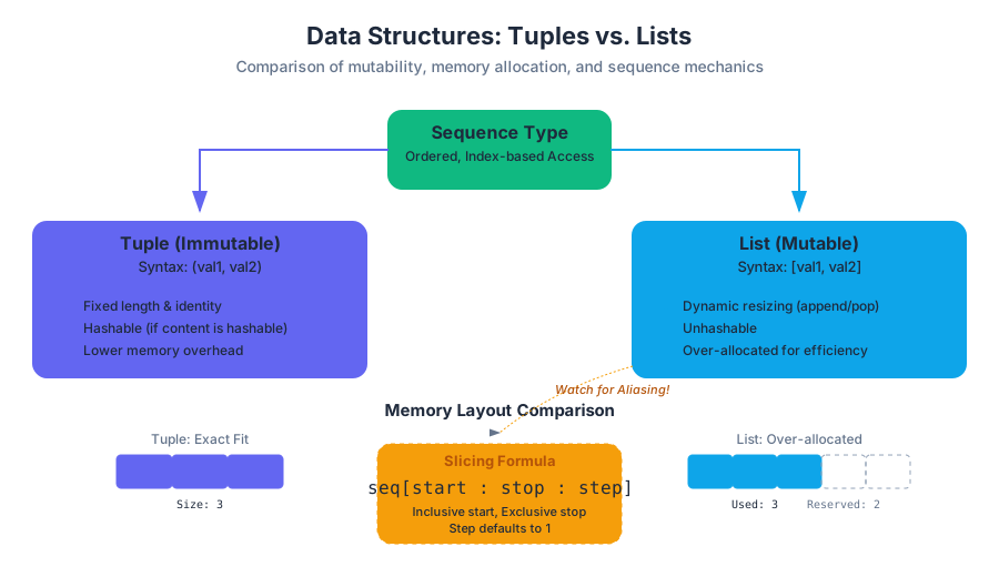
List Operations and Aliasing
Key concepts: Aliasing · Side Effects · extend() vs append() · List Sorting
Deep dive into list manipulation and the memory management concepts of aliasing.
List Operations and Aliasing
In the realm of high-level programming, particularly within Python, the distinction between objects and variable names is the most frequent source of "logic bugs" for intermediate developers. While primitive types like integers and strings are immutable—meaning their value cannot be changed in place—lists are mutable dynamic arrays. This mutability introduces a layer of complexity known as Aliasing, where multiple identifiers refer to the exact same memory location. Understanding the mechanics of how lists are stored, modified, and passed through functions is not merely an academic exercise; it is a prerequisite for writing predictable, thread-safe, and memory-efficient code.
The Architecture of Mutability
To understand list operations, one must first understand the Python memory model. In Python, a list is not a contiguous block of data values (like a C-array of integers); rather, it is a contiguous block of references to other objects. When you create a list, the Python interpreter allocates a "header" object that tracks the list's size, its allocated capacity, and a pointer to the array of references.
Definition: Mutability An object is considered mutable if its state or content can be changed after it is created without changing its identity (memory address). In Python,
list,dict, andsetare the primary mutable built-in types.
Because the list object itself stays at the same memory address even when its contents change, any variable pointing to that address will see the changes. This is the fundamental driver behind side effects.
Aliasing: The Identity Crisis
Aliasing occurs when more than one variable name is bound to the same object. In Python, the assignment operator (=) does not copy the data; it copies the reference.
Why it Matters
In a large-scale system, an alias might be created deep within a library or a helper function. If that function mutates the list, the original caller’s data is altered. This violates the principle of Least Astonishment, where a developer expects a variable to remain constant unless explicitly changed.
Mechanics and Implementation
When you execute L2 = L1, you are not creating a new list. You are creating a new entry in the local symbol table that points to the same id() (memory address) as L1.
# Block 1: Low-level implementation and identity verification
import ctypes

def get_memory_address(obj):
    """Returns the hex memory address of a Python object."""
    return hex(id(obj))

# Initialize a list
L1 = [1, 2, 3]
# Create an alias
L2 = L1

print(f"L1 Address: {get_memory_address(L1)}")
print(f"L2 Address: {get_memory_address(L2)}")
print(f"Are they the same object? {L1 is L2}")

# Mutate L1
L1.append(4)

# Observe the side effect on L2
print(f"L2 after L1 mutation: {L2}") # Output: [1, 2, 3, 4]

# Verification via C-style pointer inspection
# In CPython, id(x) is the memory address of the object
address = id(L1)
value_at_address = ctypes.cast(address, ctypes.py_object).value
print(f"Object at {hex(address)} is {value_at_address}")
To visualize this from a systems perspective, consider how this would look in a lower-level language like C, where the "aliasing" is explicitly handled via pointers.
/* Block 2: C-representation of List Aliasing */
#include <stdio.h>
#include <stdlib.h>

typedef struct {
    int *data;
    size_t size;
} PythonList;

int main() {
    // Allocate a "list"
    PythonList *L1 = malloc(sizeof(PythonList));
    L1->data = malloc(3 * sizeof(int));
    L1->size = 3;
    L1->data[0] = 1; L1->data[1] = 2; L1->data[2] = 3;

    // Aliasing: L2 is just another pointer to the same address
    PythonList *L2 = L1;

    printf("L1 Address: %p\n", (void*)L1);
    printf("L2 Address: %p\n", (void*)L2);

    // Mutating through L1 affects L2 because they share the pointer
    L1->data[0] = 99;
    printf("L2[0] value: %d\n", L2->data[0]); // Output: 99

    return 0;
}
Side Effects and Function Scope
A side effect is any change to the state of the program that occurs outside the local scope of a function, other than returning a value. Because lists are passed by assignment (often called "pass-by-object-reference"), passing a list to a function creates a local alias.
The Mutation Trap
If a function uses methods like .append(), .extend(), or .pop(), it modifies the original object. If it uses assignment like L = L + [new_item], it creates a new local object and breaks the alias, leaving the original list unchanged.
| Operation | Type | Effect on Original List | Memory Impact |
|---|---|---|---|
L.append(x) |
In-place | Mutates | Modifies existing object |
L.extend(iter) |
In-place | Mutates | Modifies existing object |
L.sort() |
In-place | Mutates | Modifies existing object |
L = L + [x] |
Assignment | No change | Creates new object |
L[:] = [x] |
Slice Assignment | Mutates | Overwrites existing object contents |
Append vs. Extend: Structural Mutation
One of the most common points of confusion for those new to Python is the difference between append() and extend(). While both increase the size of the list, they handle the input argument with different levels of "flatness."
append(object)
The append method takes a single object and adds it to the end of the list as a single element. If you append a list to another list, you create a nested structure (a list within a list).
extend(iterable)
The extend method takes an iterable (list, tuple, string, etc.) and appends each element of that iterable to the list individually. It "flattens" the input by one level.
Mathematical Derivation of Complexity
Let $L$ be the original list of size $n$, and $M$ be the input collection of size $m$.
append(M): Complexity is $O(1)$ amortized. It performs a single pointer assignment.extend(M): Complexity is $O(m)$. It must iterate through $M$ and perform $m$ assignments.
# Block 3: Performance comparison using CLI timeit
# Comparing append vs extend for building a list

# Scenario: Adding 1000 elements one by one vs adding a list of 1000 elements
python3 -m timeit -s "l = []" "for i in range(1000): l.append(i)"
python3 -m timeit -s "l = []; r = list(range(1000))" "l.extend(r)"

# Results typically show extend() is significantly faster for bulk operations
# because the resizing logic and pointer overhead happen in a single C-loop.
The Mechanics of Sorting
Python provides two ways to sort a list: the list.sort() method and the sorted() built-in function. This distinction is the quintessential example of the "In-place vs. New Object" paradigm.
list.sort()
This method sorts the list in-place. It returns None. It is highly memory efficient because it does not require a copy of the list. It uses the Timsort algorithm, which has a worst-case time complexity of $O(n \log n)$ and a space complexity of $O(n)$.
sorted(iterable)
This function takes any iterable and returns a new list containing the elements in sorted order. The original iterable remains untouched.
| Feature | list.sort() |
sorted(list) |
|---|---|---|
| Return Value | None |
A new list |
| Original List | Modified | Unchanged |
| Memory Usage | Low (In-place) | Higher (Creates copy) |
| Flexibility | Lists only | Any iterable |
The Timsort Theorem Timsort is a hybrid stable sorting algorithm, derived from merge sort and insertion sort, designed to perform well on many kinds of real-world data. It leverages "runs" of already-sorted data to minimize comparisons.
Mitigating Aliasing: Cloning and Deep Copies
To avoid the pitfalls of aliasing, a developer must clone the list. Cloning creates a new object with the same values, breaking the reference link.
Shallow Copy
A shallow copy creates a new list object, but the elements inside the list are still references to the same objects as the original.
- Syntax:
L_copy = L[:]orL_copy = L.copy()orL_copy = list(L)
Deep Copy
If a list contains other mutable objects (like nested lists), a shallow copy is insufficient. The inner lists will still be aliased. A Deep Copy recursively copies every object found in the original.
# Block 4: Shallow vs Deep Copy Edge Cases
import copy

# A nested list
original = [[1, 2], [3, 4]]

# Shallow Copy
shallow = list(original)
# Deep Copy
deep = copy.deepcopy(original)

# Mutating an inner element
original[0][0] = "CHANGED"

print(f"Original: {original}")
print(f"Shallow: {shallow}") # Output will show "CHANGED"!
print(f"Deep: {deep}")       # Output remains [[1, 2], [3, 4]]

# Conclusion: Shallow copies only copy the top-level references.
Common Pitfalls and Best Practices
- The "None" Return Trap: Beginners often write
L = L.sort(). Sincesort()returnsNone, the variableLis now destroyed, replaced byNone. - Mutable Default Arguments: Never use an empty list as a default argument in a function definition (e.g.,
def func(x, L=[])). The list is created once at definition time and aliased across every call to the function. - Iteration while Mutating: Modifying a list (adding/removing items) while iterating over it leads to skipped elements or index errors. Always iterate over a copy:
for item in L[:].
Complexity Summary Table
| Operation | Average Case | Notes |
|---|---|---|
Indexing L[i] |
$O(1)$ | Direct memory offset calculation |
Slicing L[i:j] |
$O(k)$ | Where $k$ is the slice length |
| Append | $O(1)$ | Amortized constant time |
| Insert/Delete | $O(n)$ | Requires shifting all subsequent elements |
| Sort | $O(n \log n)$ | Timsort efficiency |
Membership x in L |
$O(n)$ | Linear search |
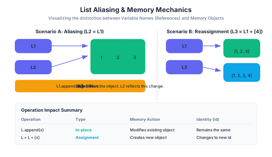
Testing and Debugging
Key concepts: Black Box Testing · Glass Box Testing · Path Completeness · Boundary Conditions
Covers strategies for ensuring code correctness and identifying logical errors.
Testing and Debugging
In the lifecycle of software development, writing code is often the easiest part. Ensuring that the code performs correctly under all possible circumstances—and identifying why it fails when it inevitably does—is the hallmark of a senior engineer. We must distinguish between two fundamental activities: Testing is the systematic process of executing a program with the intent of finding errors, while Debugging is the process of finding the cause of those errors and correcting them.
As we move from simple scripts to complex systems, our approach must shift from "trial and error" to a rigorous, scientific methodology. We do not test to prove a program is correct; as Edsger W. Dijkstra famously noted, "Program testing can be used to show the presence of bugs, but never to show their absence." Instead, we test to increase our confidence in the software's reliability.
The Philosophy of Defensive Programming
Before diving into specific testing methodologies, we must adopt the mindset of Defensive Programming. This is the practice of designing software to continue functioning under unforeseen circumstances. It involves:
- Validation: Ensuring the software meets the requirements (Are we building the right product?).
- Verification: Ensuring the software functions correctly (Are we building the product right?).
- Assertion: Using
assertstatements to document assumptions in the code that must be true for the subsequent logic to be valid.
Black Box Testing
Black Box Testing (also known as functional testing) treats the software as a "black box"—the internal implementation, data structures, and algorithms are invisible to the tester. The test cases are derived solely from the specification (the documentation describing what the code is supposed to do).
The Principle of Equivalence Partitioning
Since we cannot test every possible input (the input space is often infinite), we use Equivalence Partitioning. We divide the input data into partitions of equivalent data from which test cases can be derived. An equivalence class represents a set of inputs that the program should treat identically.
Definition: An Equivalence Class is a subset of the input domain where the behavior of the program is expected to be the same for any element within that subset. If one test case in a class uncovers an error, all other test cases in that class are likely to uncover the same error.
| Feature | Black Box Testing | Glass Box Testing |
|---|---|---|
| Focus | Requirements and Specifications | Internal Logic and Code Structure |
| Tester Knowledge | No knowledge of implementation | Full knowledge of source code |
| Goal | Validate output against input | Ensure all code paths are executed |
| Benefit | Unbiased; finds missing functions | Finds "hidden" logic errors |
| Limitation | Cannot test hidden code paths | Cannot find missing requirements |
Implementation Example: Bisection Search
Consider a function designed to find the square root of a number using the bisection method. In Black Box testing, we look at the signature and the docstring, not the while loop logic.
def find_square_root(x: float, epsilon: float = 0.01) -> float:
    """
    Computes the square root of x using bisection search.
    Precondition: x >= 0, epsilon > 0
    Returns: y such that y*y is within epsilon of x.
    """
    if x < 0:
        raise ValueError("Cannot compute square root of negative number")

    low = 0.0
    high = max(1.0, x)
    ans = (high + low) / 2.0

    while abs(ans**2 - x) >= epsilon:
        if ans**2 < x:
            low = ans
        else:
            high = ans
        ans = (high + low) / 2.0
    return ans

# Black Box Test Suite based on Specification
def test_find_square_root():
    # Test Case 1: Perfect square
    assert abs(find_square_root(16.0) - 4.0) < 0.01
    # Test Case 2: Float input
    assert abs(find_square_root(0.25) - 0.5) < 0.01
    # Test Case 3: Large number
    assert abs(find_square_root(1000000.0) - 1000.0) < 0.01
    # Test Case 4: Boundary (Zero)
    assert abs(find_square_root(0.0) - 0.0) < 0.01
Glass Box Testing
Glass Box Testing (or White Box Testing) uses the internal structure of the code to design test cases. The goal is to ensure that the "plumbing" of the program is sound. We look at the control flow graph of the program and attempt to achieve various levels of coverage.
Path Completeness
A test suite is said to be Path Complete if it exercises every possible path through the program's control flow. This is the gold standard of Glass Box testing, but it is often unattainable in practice due to loops and complex branching.
- Statement Coverage: Every line of code is executed at least once.
- Branch Coverage: Every outcome of every decision point (e.g., both the
TrueandFalsebranches of anifstatement) is executed. - Path Coverage: Every distinct sequence of statements from the start to the end of the function is executed.
Complexity of Path Coverage
For a program with $n$ sequential if statements, there are $2^n$ possible paths. If a program contains a loop that can run up to $k$ times, and there are $m$ paths inside the loop, the number of paths grows exponentially ($m^k$). This is known as Path Explosion.
ALGORITHM: CalculatePathComplexity(ControlFlowGraph G)
    1. Identify all decision nodes (if, while, for, switch)
    2. For each node, count the number of outgoing edges (e)
    3. Cyclomatic Complexity M = E - N + 2P
       where:
       E = number of edges
       N = number of nodes
       P = number of connected components (usually 1)
    4. RETURN M (The minimum number of tests for branch coverage)
Boundary Conditions
Errors rarely occur in the "middle" of an input range. They cluster at the Edges. Boundary condition testing focuses on the values at the limits of the input domain, just inside and just outside the boundaries.
Common Boundary Categories
When testing a function, you should always consider the following "Stress" inputs:
- Numeric:
0,1,-1,max_int,min_int,float.epsilon,NaN,Infinity. - Collections (Lists/Strings): Empty list
[], empty string"", single element, duplicate elements, very large collections. - Types: Passing a float where an integer is expected, or
Nonewhere an object is expected.
| Data Type | Boundary Test Cases | Logic to Check |
|---|---|---|
| Integers | 0, 1, -1, 2^31-1, -2^31 |
Overflow, off-by-one errors, division by zero |
| Floats | 0.0, 1e-7, 1e30, NaN |
Precision loss, epsilon comparison errors |
| Strings | "", " ", \0, very long strings |
Null terminators, whitespace handling, memory allocation |
| Lists | [], [x], [x, x, x] |
Indexing errors, empty iteration, aliasing |
The Danger of Off-by-One Errors (OBOE)
In C-style languages, boundary conditions often manifest as buffer overflows. If a loop runs from 0 to n instead of 0 to n-1, it accesses memory outside the allocated bounds.
#include <stdio.h>

// A classic boundary condition failure: Buffer Overflow
void vulnerable_function(int *arr, int size) {
    // If size is 10, and we loop <= size, we hit the 11th element (index 10)
    for (int i = 0; i <= size; i++) {
        arr[i] = i * 2; // Potential memory corruption at arr[size]
    }
}

int main() {
    int data[10];
    vulnerable_function(data, 10); // Boundary error triggered here
    return 0;
}
The Debugging Process: A Scientific Approach
When a test fails, we move into the Debugging phase. Debugging is not a random walk through the code; it is an application of the Scientific Method.
- Study the Data: Examine the failing test case and the resulting error message (the symptom).
- Form a Hypothesis: Propose a reason for the failure that is consistent with all observed data.
- Design an Experiment: Create a small, repeatable test case that would prove or disprove the hypothesis.
- Execute and Observe: Run the experiment. If the hypothesis is disproved, return to step 2.
- Fix and Verify: Once the root cause is found, fix it and run all previous tests (Regression Testing) to ensure no new bugs were introduced.
Binary Search Debugging
If you have a large block of code and don't know where the error lies, use Binary Search. Comment out half the code. Does the error persist? If yes, the bug is in the remaining half. If no, it was in the commented-out half. Repeat this until you isolate the specific line.
Tools of the Trade
Modern debugging relies on more than just print statements.
| Tool Type | Example | Purpose |
|---|---|---|
| Interactive Debugger | pdb, gdb, VS Code Debugger |
Set breakpoints, step through code, inspect variable state |
| Unit Test Framework | pytest, JUnit, Mocha |
Automate the execution of test suites |
| Linters / Static Analysis | pylint, ESLint, SonarQube |
Catch syntax and stylistic errors before execution |
| Profilers | cProfile, Valgrind |
Identify performance bottlenecks and memory leaks |
Automation with Pytest
In professional environments, we use CLI tools to run hundreds of tests in seconds. This ensures that a fix for one bug doesn't break a different feature.
# Running tests with coverage reporting
$ pytest --cov=my_project tests/

# Output:
# ========================= test session starts =========================
# platform linux -- Python 3.9.1, pytest-6.2.2
# rootdir: /home/user/project
# collected 45 items
#
# tests/test_math.py ......................................... [ 91%]
# tests/test_api.py ....                                       [100%]
#
# ----------- coverage: platform linux, python 3.9.1 -----------
# Name                 Stmts   Miss  Cover
# ----------------------------------------
# my_project/math.py      50      2    96%
# my_project/api.py      120     15    88%
# ----------------------------------------
# TOTAL                  170     17    90%
# ========================= 45 passed in 0.82s =========================
Integration and Regression Testing
Once individual functions (units) are tested, we must perform Integration Testing to ensure that different modules work together. A function might work perfectly in isolation but fail when passed a specific object type from another module.
Finally, we perform Regression Testing. Every time a bug is fixed, the test case that uncovered that bug should be added to the permanent test suite. This prevents the bug from "re-emerging" in future versions of the software—a surprisingly common occurrence in large-scale engineering.
Key Insight: The goal of debugging is not just to make the error go away, but to understand why the error occurred. If you fix a bug by "tweaking" the code until it works without understanding the underlying logic, you are likely just hiding the symptom while the disease remains.
Summary of Best Practices
- Test Early, Test Often: It is much cheaper to find a bug during development than after deployment.
- Write Tests for the Specification, not the Code: This ensures your tests remain valid even if you rewrite the internal implementation.
- Automate: If a test isn't automated, it won't be run.
- Isolate: Use "Mocks" or "Stubs" to isolate the unit you are testing from external dependencies like databases or APIs.
- Document: A test case is a form of documentation. It tells the next engineer exactly how the code is expected to behave.
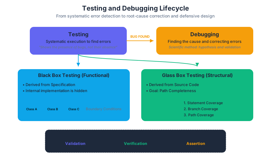
Exception Handling and Errors
Key concepts: TypeError · try/except blocks · Runtime Errors · Input Validation
Explains how to handle runtime errors gracefully using Python's error-handling blocks.
Exception Handling and Errors
In the lifecycle of software development, the "Happy Path"—the sequence of execution where everything goes exactly as planned—is often the shortest part of the story. Real-world computing is messy. Networks fail, users provide malformed input, and hardware resources are exhausted. To build resilient systems, a programmer must move beyond writing code that works to writing code that fails gracefully.
Exception handling is the architectural discipline of managing these deviations. It is not merely a way to "stop the crash"; it is a control flow mechanism that allows a program to preserve its state, clean up resources, and provide meaningful feedback when the unexpected occurs.
The Taxonomy of Errors: Syntax vs. Runtime vs. Semantic
Before mastering the try/except block, we must distinguish between the different categories of "broken" code. Not all errors are created equal, and not all can be caught by the program itself.
| Error Category | Discovery Phase | Definition | Example |
|---|---|---|---|
| Syntax Error | Parsing/Compile Time | The code violates the formal grammar of the language. | if x = 5: (missing = for comparison) |
| Runtime Error (Exception) | Execution Time | The code is syntactically correct but encounters an illegal operation during run. | 10 / 0 (ZeroDivisionError) |
| Semantic (Logic) Error | Post-Execution | The program runs without crashing but produces the wrong output. | Using + instead of * in a formula. |
The Exception Axiom: An exception is an event that occurs during the execution of a program that disrupts the normal flow of instructions. When an error occurs within a method, the method creates an object—the Exception Object—and hands it off to the runtime system.
The Mechanics of the Try-Except Block
The primary mechanism for handling runtime errors is the try/except block. In Python, this follows the philosophy of EAFP (Easier to Ask for Forgiveness than Permission), contrasting with the LBYL (Look Before You Leap) approach common in languages like C.
The Control Flow Pipeline
- The
tryblock: The interpreter attempts to execute the code within this scope. - The Exception Trigger: If an error occurs, execution of the
tryblock stops immediately. - The Handler Search: The interpreter looks for an
exceptblock that matches the type of exception raised. - The
exceptblock: If a match is found, the code inside the handler executes. - The
elseblock (Optional): Executes only if thetryblock succeeded without any exceptions. - The
finallyblock (Optional): Executes regardless of whether an exception occurred, typically used for resource cleanup (closing files, releasing database locks).
Implementation: Robust Data Processing
The following Python implementation demonstrates a sophisticated handler for processing a list of mixed data types, a common task in data engineering where "dirty data" is the norm.
def process_sensor_data(data_list):
    """
    Processes a list of raw sensor readings.
    Handles TypeErrors and ValueErrors while ensuring system integrity.
    """
    results = []
    for record in data_list:
        try:
            # Attempt to normalize and cast the data
            # Potential TypeError: record is not a string/number
            # Potential ValueError: string cannot be converted to float
            normalized_val = float(record)

            if normalized_val < 0:
                raise ValueError(f"Negative reading encountered: {normalized_val}")

            results.append(normalized_val ** 2)

        except TypeError as te:
            print(f"[CRITICAL] Incompatible data type: {type(record)}. Error: {te}")
            continue # Skip to next record

        except ValueError as ve:
            print(f"[WARNING] Skipping invalid value '{record}': {ve}")
            continue

        except Exception as e:
            # Catch-all for unforeseen issues (e.g., MemoryError)
            print(f"[FATAL] Unexpected error: {e}")
            raise # Re-raise the exception to be handled by the caller

        else:
            # This runs if the try block succeeded
            print(f"Successfully processed: {record}")

        finally:
            # This runs every iteration, used here for telemetry
            print("Cleanup: Ready for next record.")

    return results

# Example invocation
data = ["10.5", "20", "invalid_str", None, -5.2]
print(process_sensor_data(data))
The Logic of Propagation: The Call Stack
When an exception is raised and not caught within the current function, it "bubbles up" the call stack. This is known as Exception Propagation. If the exception reaches the entry point of the program (the global scope) without being caught, the interpreter terminates the program and prints a Traceback.
Mathematical Representation of Exception Propagation
Let $F_n$ be a sequence of function calls where $F_0$ is the main entry point. If an exception $\epsilon$ occurs at $F_k$:
- If $F_k$ has a handler for $\epsilon$, it is resolved.
- If not, $F_k$ is popped from the stack, and $\epsilon$ is passed to $F_{k-1}$.
- This continues until $k=0$. If $F_0$ has no handler, the program state $\Sigma$ is terminated.
ALGORITHM: ExceptionPropagation(Exception e, Stack s)
    WHILE s is NOT empty:
        f = s.peek()
        IF f.hasHandler(e):
            f.executeHandler(e)
            RETURN
        ELSE:
            s.pop()
    TERMINATE_PROGRAM(e.traceback)
TypeError: The Sentinel of Type Safety
A TypeError is one of the most frequent exceptions in Python. It occurs when an operation or function is applied to an object of an inappropriate type. Because Python is dynamically typed, it does not check types until the code actually runs.
Common Triggers for TypeError
- Unsupported Operand Types: Trying to add a string to an integer (
"5" + 5). - Inappropriate Iteration: Trying to loop over a non-iterable object (e.g.,
for x in 100:). - Incorrect Function Arguments: Passing the wrong number of arguments or an object that the function cannot process (e.g.,
len(5)).
| Operation | Cause of TypeError | Corrective Action |
|---|---|---|
len(1024) |
Integers have no __len__ method. |
Convert to string: len(str(1024)) |
'Age: ' + 25 |
Cannot concatenate str and int. |
Explicit cast: 'Age: ' + str(25) |
math.sqrt('9') |
sqrt expects a float/int. |
Cast input: math.sqrt(float('9')) |
Input Validation and Defensive Programming
Defensive programming is the practice of anticipating failure. While try/except handles errors after they happen, Input Validation seeks to prevent them from occurring in the first place.
LBYL vs. EAFP
In the LBYL (Look Before You Leap) style, you check conditions explicitly before performing an operation. In EAFP (Easier to Ask for Forgiveness than Permission), you assume the operation will work and catch the fallout if it doesn't.
| Feature | LBYL (Look Before You Leap) | EAFP (Ask Forgiveness) |
|---|---|---|
| Philosophy | Pre-emptive checking. | Reactive handling. |
| Performance | Slower if checks are redundant. | Faster on the "Happy Path." |
| Readability | Can lead to "if-nesting" hell. | Cleaner, logic-focused code. |
| Concurrency | Risk of TOCTOU (Time-of-check to time-of-use) bugs. | Thread-safe for atomic operations. |
Real-World Usage: CLI and Environment Validation
In systems programming, we often deal with external environments (files, network ports) where LBYL is dangerous due to race conditions. Here, EAFP is the gold standard.
# A shell script demonstrating manual error code checking (The C/Unix style)
# This is the "Look Before You Leap" equivalent in systems scripting.

FILE="/etc/config_data.json"

if [[ -f "$FILE" ]]; then
    echo "File exists, attempting to read..."
    # Attempt to read; even if it exists, it might be unreadable (permissions)
    cat "$FILE"
    if [[ $? -ne 0 ]]; then
        echo "Error: Read failed despite file existence." >&2
        exit 1
    fi
else
    echo "Error: Configuration file missing." >&2
    exit 1
fi
Raising Exceptions and Custom Errors
As a developer, you are not limited to catching built-in exceptions; you can also raise them to signal that your code has reached an invalid state. Furthermore, for complex applications, defining Custom Exception Classes allows you to categorize errors specific to your domain (e.g., InsufficientFundsError in a banking app).
Custom Exceptions in Object-Oriented Programming
By inheriting from the base Exception class, you create a new type that can be caught specifically by your application's error-handling logic.
class ValidationError(Exception):
    """Base class for validation errors in this module."""
    pass

class PasswordTooShortError(ValidationError):
    """Raised when the password does not meet minimum length."""
    def __init__(self, length, minimum=8):
        self.length = length
        self.minimum = minimum
        super().__init__(f"Password length {length} is less than {minimum}")

def register_user(username, password):
    if len(password) < 8:
        raise PasswordTooShortError(len(password))
    print(f"User {username} registered successfully.")

try:
    register_user("alice", "123")
except PasswordTooShortError as e:
    print(f"Registration failed: {e}")
Common Pitfalls and Best Practices
- The "Silent Killer" (Bare Except): Using
except:without specifying an exception type. This catches everything, includingKeyboardInterrupt(Ctrl+C), making it impossible to stop the program.- Fix: Always catch specific exceptions (
except ValueError:).
- Fix: Always catch specific exceptions (
- Over-Handling: Wrapping your entire program in one giant
tryblock. This obscures where the error actually occurred.- Fix: Keep
tryblocks as small as possible, covering only the lines that are likely to fail.
- Fix: Keep
- Ignoring the Traceback: Catching an exception and printing a generic "Error occurred" message.
- Fix: Use
logging.exception()to record the full stack trace for debugging.
- Fix: Use
- Resource Leaks: Opening a file in a
tryblock but forgetting to close it in theexceptblock.- Fix: Use the
finallyblock or, better yet, Context Managers (withstatements).
- Fix: Use the
Summary of Built-in Exceptions
| Exception | Meaning |
|---|---|
AttributeError |
Attempting to access a non-existent attribute of an object. |
IndexError |
Sequence subscript is out of range. |
KeyError |
Dictionary key is not found. |
NameError |
Local or global name is not defined. |
RuntimeError |
A general error that doesn't fit other categories. |
StopIteration |
Raised by next() to signal that an iterator has no more items. |
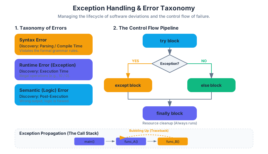
Recursion, Efficiency, and OOP
Key concepts: Recursion · Algorithmic Efficiency · Object-Oriented Programming (OOP) · Data Structures (Dictionaries)
An introduction to more complex computer science topics including recursive functions and object-oriented design.
Recursion, Efficiency, and OOP
The transition from writing "scripts" to engineering "software" is marked by a fundamental shift in how a programmer perceives data and control flow. In the early stages of learning, we focus on imperative logic—telling the computer exactly what to do, step-by-step. However, as the complexity of problems scales, these linear approaches become brittle and inefficient.
To build robust systems, we must master three pillars of advanced computation: Recursion (a functional approach to decomposition), Algorithmic Efficiency (the mathematical rigor of performance), and Object-Oriented Programming (the architectural paradigm of data encapsulation). Interlinking these is the Dictionary, a data structure that serves as the backbone for high-performance data retrieval.
The Power of Mapping: Dictionaries and Associative Arrays
In Python, the Dictionary (dict) is arguably the most important built-in data structure. Unlike a list, which is an ordered collection indexed by integers, a dictionary is an associative array. It maps unique keys to specific values.
What it is
A dictionary is a collection of key-value pairs where each key must be hashable (immutable). Mathematically, it represents a function $f: K \to V$, where $K$ is the set of keys and $V$ is the set of values.
Why it matters
The primary motivation for using dictionaries is lookup speed. In a list of $n$ elements, finding a specific item requires, on average, searching through $n/2$ items—an $O(n)$ operation. In a dictionary, the time complexity for a lookup is effectively $O(1)$, or constant time, regardless of how many millions of items are stored.
| Feature | List (list) |
Dictionary (dict) |
|---|---|---|
| Access Method | Integer Index (0, 1, 2...) | Unique Key (String, Int, Tuple) |
| Ordering | Ordered (Maintains insertion sequence) | Unordered (Python 3.7+ maintains insertion, but logic is key-based) |
| Lookup Speed | $O(n)$ (Linear search) | $O(1)$ (Hash table lookup) |
| Mutability | Mutable | Mutable |
| Common Use Case | Sequences, Stacks, Queues | Databases, JSON-like structures, Frequency counters |
How it works: The Hash Table
Under the hood, Python dictionaries use a Hash Table. When you provide a key, Python applies a hash function to transform that key into an integer. This integer corresponds to an index in a hidden array. This allows the computer to jump directly to the memory location of the value without scanning the entire structure.
# First code block: Low-level implementation of a frequency counter
# This demonstrates the efficiency of O(1) lookups in a real-world scenario

def analyze_word_frequency(text: str) -> dict:
    """
    Analyzes a block of text and returns a dictionary of word counts.
    Demonstrates the 'Get-and-Update' pattern common in data processing.
    """
    clean_text = text.lower().replace('.', '').replace(',', '')
    words = clean_text.split()

    frequency_map = {}

    for word in words:
        # The dictionary lookup happens in O(1) time
        if word in frequency_map:
            frequency_map[word] += 1
        else:
            frequency_map[word] = 1

    return frequency_map

# Example usage
sample_data = "Recursion is powerful. Efficiency is vital. OOP is structural."
print(analyze_word_frequency(sample_data))
Common Pitfalls
- KeyErrors: Attempting to access a key that does not exist. Use
.get(key, default)to handle missing keys gracefully. - Mutable Keys: You cannot use a list as a dictionary key because lists are mutable. If the list changes, its hash would change, making the value unretrievable.
Recursion: The "Divide and Conquer" Philosophy
Recursion is a method of solving a problem where the solution depends on solutions to smaller instances of the same problem. It is the programmatic implementation of Mathematical Induction.
The Anatomy of a Recursive Function
Every valid recursive function must possess two components:
- The Base Case: The simplest possible instance of the problem, which can be solved directly without further recursion. This prevents infinite loops (and the dreaded
RecursionError: maximum recursion depth exceeded). - The Recursive Step: The part of the function where the problem is reduced in size and the function calls itself.
The Recursive Leap of Faith: To write a recursive function, assume that the recursive call to the smaller problem "just works." Your only job is to handle the base case and combine the result of the smaller problem into the solution for the current problem.
Mathematical Derivation: The Factorial
The factorial of $n$ (denoted $n!$) is defined as: $n! = n \times (n-1) \times (n-2) \times \dots \times 1$
This can be expressed recursively as: $$ f(n) = \begin{cases} 1 & \text{if } n = 0 \text{ or } 1 \text{ (Base Case)} \ n \times f(n-1) & \text{if } n > 1 \text{ (Recursive Step)} \end{cases} $$
// Second code block: Pseudocode and Logic Flow
// Visualizing the Call Stack for factorial(3)

FUNCTION factorial(n):
    IF n == 1:
        RETURN 1  // Base case reached
    ELSE:
        // Recursive step: n * (n-1)!
        RESULT = n * factorial(n - 1)
        RETURN RESULT

/*
Stack Execution Trace:
1. factorial(3) calls factorial(2) -> waits
2. factorial(2) calls factorial(1) -> waits
3. factorial(1) returns 1          -> resolves
4. factorial(2) receives 1, returns 2 * 1 = 2
5. factorial(3) receives 2, returns 3 * 2 = 6
*/
Recursion vs. Iteration
While any recursive algorithm can be written iteratively (using loops), recursion is often more intuitive for problems involving hierarchical data (trees, graphs) or combinatorial problems (Towers of Hanoi, Permutations).
| Aspect | Recursion | Iteration |
|---|---|---|
| Implementation | Function calls itself | for or while loops |
| State | Stored in the Call Stack | Stored in local variables |
| Memory | High (each call adds a stack frame) | Low (constant space overhead) |
| Readability | Often cleaner for complex logic | Generally more straightforward for simple loops |
Algorithmic Efficiency: Big O Notation
As a computer scientist, it is not enough to know that a program works; you must know how well it scales. Algorithmic Efficiency is the study of how the execution time and memory requirements of an algorithm grow as the input size ($n$) increases.
Big O Notation ($O$)
We use Big O Notation to describe the upper bound of an algorithm's complexity. It ignores constants and lower-order terms to focus on the "order of growth."
Common Complexity Classes
| Notation | Name | Description | Example |
|---|---|---|---|
| $O(1)$ | Constant | Time does not change with input size. | Dictionary lookup, array indexing. |
| $O(\log n)$ | Logarithmic | Input size is halved each step. | Binary Search. |
| $O(n)$ | Linear | Time grows proportionally to input. | Simple loop through a list. |
| $O(n \log n)$ | Log-Linear | Efficient sorting. | Merge Sort, Quick Sort. |
| $O(n^2)$ | Quadratic | Nested loops. | Bubble Sort, comparing all pairs. |
| $O(2^n)$ | Exponential | Doubling with each addition. | Recursive Fibonacci (without memoization). |
Why Constants Don't Matter
In Big O, $O(2n)$ and $O(100n)$ are both simplified to $O(n)$. This is because, as $n$ approaches infinity, the multiplicative constant becomes insignificant compared to the growth of $n$ itself. We are interested in the asymptotic behavior.
# Third code block: Real-world performance profiling
# Using the 'timeit' module to compare O(n) vs O(1)

# Comparing list search vs dictionary search for 1,000,000 elements
python3 -m timeit -s "data = list(range(1000000))" "999999 in data"
# Result: ~10-20 milliseconds (Linear Search)

python3 -m timeit -s "data = {i: i for i in range(1000000)}" "999999 in data"
# Result: ~0.00005 milliseconds (Hash Lookup)
Object-Oriented Programming (OOP): The Architecture of Data
Object-Oriented Programming is a paradigm based on the concept of "objects," which can contain data (attributes) and code (methods). It is designed to manage the complexity of large software systems by grouping related data and behaviors together.
The Four Pillars of OOP
- Encapsulation: Bundling data and methods that work on that data within a single unit (a class) and restricting access to some of the object's components.
- Abstraction: Hiding complex implementation details and showing only the necessary features of an object.
- Inheritance: A mechanism where a new class (subclass) inherits properties and behaviors from an existing class (superclass).
- Polymorphism: The ability of different classes to be treated as instances of the same general class through the same interface (e.g., a
Circleand aSquareboth having an.area()method).
Classes vs. Instances
A Class is a blueprint (e.g., the concept of a "Car"). An Instance is a specific object created from that blueprint (e.g., "Your 2022 Blue Toyota").
// Fourth code block: OOP Implementation in Java
// Demonstrating Inheritance and Encapsulation

// Superclass
class Employee {
    private String name; // Encapsulation: private variable
    protected double salary;

    public Employee(String name, double salary) {
        this.name = name;
        this.salary = salary;
    }

    public void work() {
        System.out.println(name + " is working...");
    }
}

// Subclass inheriting from Employee
class Developer extends Employee {
    private String language;

    public Developer(String name, double salary, String language) {
        super(name, salary); // Call superclass constructor
        this.language = language;
    }

    @Override
    public void work() {
        System.out.println("Coding in " + language);
    }
}
Method Resolution and self
In Python, every method in a class must take self as its first argument. self refers to the specific instance of the object being manipulated. When you call my_object.method(), Python automatically passes my_object as the self argument.
| Term | Definition |
|---|---|
| Attribute | A variable belonging to an object (e.g., car.color). |
| Method | A function belonging to an object (e.g., car.drive()). |
| Constructor | A special method (__init__ in Python) called when an object is instantiated. |
| Super | A keyword used to access methods or constructors from a parent class. |
Integrating the Concepts: A Case Study in Efficiency
Consider the problem of calculating the $n$-th Fibonacci number. A naive recursive solution has a complexity of $O(2^n)$ because it recalculates the same values thousands of times.
- Recursion: Provides the logic ($fib(n) = fib(n-1) + fib(n-2)$).
- Dictionaries: Can be used for Memoization (storing previously calculated results).
- Efficiency: Memoization turns an $O(2^n)$ problem into an $O(n)$ problem.
- OOP: We can wrap this logic in a
FibonacciCalculatorclass to encapsulate the cache.
The Memoization Pattern
By checking a dictionary before performing a recursive calculation, we eliminate redundant work. This is a classic example of the Space-Time Tradeoff: we use a little more memory (the dictionary) to gain a massive increase in speed.
# Final Example: Optimized Recursive OOP
class FibonacciCalculator:
    def __init__(self):
        # Dictionary to store calculated values (Memoization)
        self.cache = {0: 0, 1: 1}

    def get_fib(self, n: int) -> int:
        # O(1) check in dictionary
        if n in self.cache:
            return self.cache[n]

        # Recursive step
        self.cache[n] = self.get_fib(n - 1) + self.get_fib(n - 2)
        return self.cache[n]

calc = FibonacciCalculator()
print(calc.get_fib(100)) # This would take centuries without the dictionary
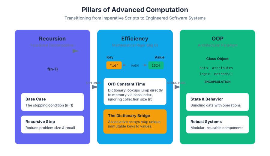
Source Materials
- Introduction to Computer Science and Programming in Python
- Introduction to Computer Science and Programming in Python
- Introduction to Computer Science and Programming in Python
- Introduction to Computer Science and Programming in Python
- Introduction to Computer Science and Programming in Python
- Introduction to Computer Science and Programming in Python
- Introduction to Computer Science and Programming in Python
- Introduction to Computer Science and Programming in Python
- Download transcript
- Download transcript
Study Introduction to Computer Science and Programming in Python with AI — Free on Lykke
Sign up for free to generate personalized flashcards, quizzes, and study guides from this course. Chat with an AI tutor that knows the material.
Get Started FreeView this course wiki on Lykke · Browse all public course wikis