High School Physics
Institution: MIT
42 study materials · 12 sections
The Client Challenge course is a comprehensive high school physics program designed to build mastery in classical mechanics, wave phenomena, and electromagnetism. The curriculum spans ten core units, starting with the fundamentals of one-dimensional motion and progressing through complex topics like Newton's laws, energy conservation, and DC circuits. By integrating mathematical analysis with conceptual understanding, the course prepares students for advanced scientific study through rigorous assessments and practical problem-solving exercises.
Course Sections
Fundamentals of One-Dimensional Motion
Key concepts: Displacement and Distance · Average and Instantaneous Velocity · Acceleration · Free Fall
An introduction to the basic descriptors of motion, focusing on displacement, velocity, and acceleration in a single dimension.
Fundamentals of One-Dimensional Motion
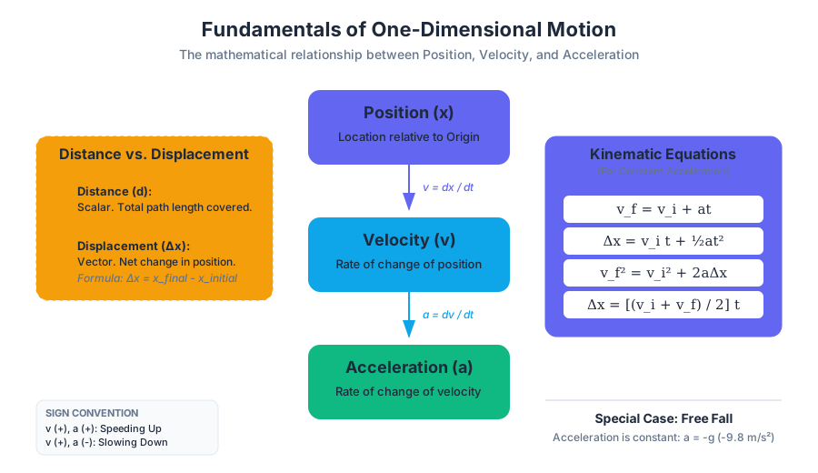
Kinematics is the branch of classical mechanics that describes the motion of points, bodies, and systems of bodies without considering the forces that cause the motion. In its simplest form—One-Dimensional Motion—we constrain the movement of an object to a single straight line. This simplification allows us to build a rigorous mathematical framework using scalars and vectors, providing the essential groundwork for more complex multi-dimensional dynamics.
Displacement and Distance
The study of motion begins with the definition of position. To describe where an object is, we must first establish a Frame of Reference and an Origin. Once a coordinate system is defined, we can distinguish between the total path traveled and the net change in position.
Distance ($d$)
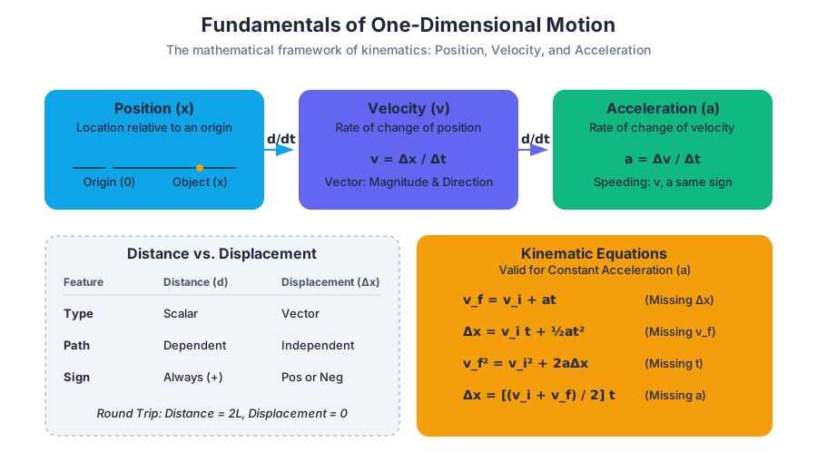
Distance is a scalar quantity that refers to "how much ground an object has covered" during its motion. It is always non-negative and is path-dependent. If you walk 5 meters forward and 3 meters backward, your total distance is 8 meters.
Displacement ($\Delta x$)
Displacement is a vector quantity that refers to "how far out of place an object is"; it is the object's overall change in position. It is path-independent and depends only on the initial and final positions.
The Displacement Formula: $$\Delta x = x_f - x_i$$ Where $x_f$ is the final position and $x_i$ is the initial position.
| Feature | Distance ($d$) | Displacement ($\Delta x$) |
|---|---|---|
| Quantity Type | Scalar (Magnitude only) | Vector (Magnitude and Direction) |
| Path Dependency | Dependent on the actual path taken | Independent (only start and end matter) |
| Sign | Always positive or zero | Can be positive, negative, or zero |
| SI Unit | Meters (m) | Meters (m) |
Common Pitfall: The Round Trip
A common point of confusion occurs in "round trip" scenarios. If an athlete runs one full lap around a 400m track, their distance is 400m, but their displacement is 0m because their initial and final positions are identical. In 1D motion, this is represented by moving from $x=0$ to $x=10$ and back to $x=0$.
Average and Instantaneous Velocity
While displacement tells us the "what" of motion, velocity tells us the "how fast" and "in what direction."
Average Velocity vs. Average Speed
Average Velocity ($v_{avg}$) is the rate at which an object changes its position over a specific time interval. Average Speed is the total distance traveled divided by the time interval.
$$v_{avg} = \frac{\Delta x}{\Delta t} = \frac{x_f - x_i}{t_f - t_i}$$
Instantaneous Velocity
Instantaneous Velocity is the velocity of an object at a specific point in time. Mathematically, it is the limit of the average velocity as the time interval approaches zero. In the language of calculus, velocity is the first derivative of position with respect to time.
$$v(t) = \lim_{\Delta t \to 0} \frac{\Delta x}{\Delta t} = \frac{dx}{dt}$$
Implementation: Numerical Differentiation of Position Data
In engineering and data science, we often work with discrete position samples rather than continuous functions. The following Python example demonstrates how to calculate instantaneous velocity from a noisy set of position data using NumPy.
import numpy as np

def calculate_velocity(time_array, position_array):
    """
    Calculates instantaneous velocity using central differences.
    For a position vector X and time vector T, v[i] = (X[i+1] - X[i-1]) / (T[i+1] - T[i-1])
    """
    if len(time_array) != len(position_array):
        raise ValueError("Time and position arrays must have the same length.")

    # Calculate differences between adjacent elements
    dt = np.diff(time_array)
    dx = np.diff(position_array)

    # Simple forward difference for velocity
    # v = dx / dt
    velocity = dx / dt

    # To maintain array length, we can pad or use central difference
    # Here we return the velocity at the midpoints of the intervals
    return velocity

# Example usage: A car moving with x(t) = t^2
t = np.linspace(0, 10, 100)
x = t**2
v_calc = calculate_velocity(t, x)

print(f"Calculated velocity at t=5s: {v_calc[50]:.2f} m/s")
print(f"Theoretical velocity (2t) at t=5s: 10.00 m/s")
Acceleration
Acceleration ($a$) is the rate at which an object changes its velocity. Because velocity is a vector, acceleration occurs if the object changes its speed, its direction, or both. In 1D motion, direction change is limited to a sign flip (positive to negative).
Mathematical Derivation
Acceleration is the derivative of velocity with respect to time, which also makes it the second derivative of position.
v(t) = \frac{dx}{dt}
a(t) = \frac{dv}{dt} = \frac{d^2x}{dt^2}
Constant vs. Variable Acceleration
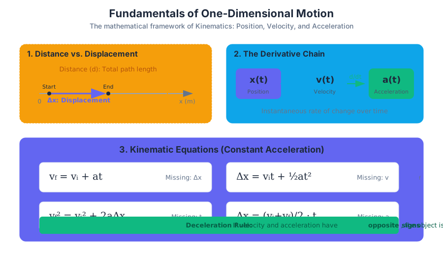
Most introductory physics problems assume Constant Acceleration (Uniformly Accelerated Motion). This allows us to derive the "Kinematic Equations," a suite of formulas that link displacement, initial velocity, final velocity, acceleration, and time.
| Equation | Missing Variable | Condition |
|---|---|---|
| $v_f = v_i + at$ | $\Delta x$ | Constant $a$ |
| $\Delta x = v_i t + \frac{1}{2}at^2$ | $v_f$ | Constant $a$ |
| $v_f^2 = v_i^2 + 2a\Delta x$ | $t$ | Constant $a$ |
| $\Delta x = \frac{v_i + v_f}{2}t$ | $a$ | Constant $a$ |
Deceleration vs. Negative Acceleration
A critical conceptual hurdle is the distinction between "slowing down" and "negative acceleration."
- If velocity and acceleration have the same sign (both positive or both negative), the object is speeding up.
- If velocity and acceleration have opposite signs, the object is slowing down (decelerating).
Free Fall
Free Fall is a specific type of one-dimensional motion where the only force acting upon an object is gravity. In a vacuum (ignoring air resistance), all objects fall toward the center of the Earth with the same constant acceleration, regardless of their mass.
The Acceleration due to Gravity ($g$)
On the surface of the Earth, this acceleration is approximately: $$g \approx 9.81 , \text{m/s}^2$$ By convention, if we define "up" as the positive y-direction, then the acceleration for an object in free fall is $a = -g$.
Worked Example: The Cliff Diver
A diver drops from a cliff that is 20 meters high. How long does it take to hit the water, and what is their impact velocity?
- Identify Knowns: $y_i = 20m$, $y_f = 0m$, $v_i = 0$ (dropped), $a = -9.8m/s^2$.
- Find Time ($t$): Use $\Delta y = v_i t + \frac{1}{2}at^2$ $-20 = 0 + \frac{1}{2}(-9.8)t^2$ $-20 = -4.9t^2 \implies t^2 \approx 4.08 \implies t \approx 2.02 , \text{s}$
- Find Final Velocity ($v_f$): Use $v_f = v_i + at$ $v_f = 0 + (-9.8)(2.02) = -19.8 , \text{m/s}$
Real-World Usage: Physics Engine Integration
In game development or robotics simulation, we use numerical integration to solve for free fall in real-time. The most common method is Euler Integration, though more stable methods like Verlet are preferred for precision.
// Simple Euler Integration for 1D Free Fall in C++
#include <iostream>

struct RigidBody1D {
    double position;
    double velocity;
    double acceleration;
};

void update_physics(RigidBody1D &body, double deltaTime) {
    // Standard gravity constant
    const double g = -9.81;
    body.acceleration = g;

    // Update velocity: v = v0 + a*dt
    body.velocity += body.acceleration * deltaTime;

    // Update position: x = x0 + v*dt
    body.position += body.velocity * deltaTime;
}

int main() {
    RigidBody1D ball = {100.0, 0.0, 0.0}; // Start at 100m
    double dt = 0.1; // 100ms steps

    for (int i = 0; i < 50; ++i) {
        update_physics(ball, dt);
        if (ball.position <= 0) {
            std::cout << "Impact at step " << i << std::endl;
            break;
        }
        std::cout << "Time: " << i*dt << "s | Height: " << ball.position << "m" << std::endl;
    }
    return 0;
}
Graphical Analysis of Motion
Visualizing motion through graphs is often more intuitive than algebraic manipulation. There are three primary types of motion graphs:
1. Position vs. Time ($x-t$)
- Slope: Represents the velocity.
- Curvature: A curved line indicates acceleration. A straight line indicates constant velocity.
- Y-Intercept: The initial position ($x_i$).
2. Velocity vs. Time ($v-t$)
- Slope: Represents the acceleration.
- Area Under Curve: Represents the displacement ($\Delta x$).
- Horizontal Line: Indicates constant velocity (zero acceleration).
3. Acceleration vs. Time ($a-t$)
- Slope: Represents "jerk" (rate of change of acceleration).
- Area Under Curve: Represents the change in velocity ($\Delta v$).
| Graph Type | Slope Meaning | Area Meaning |
|---|---|---|
| Position-Time | Velocity | N/A |
| Velocity-Time | Acceleration | Displacement |
| Acceleration-Time | Jerk | Change in Velocity |
Advanced Considerations: Non-Uniform Acceleration
In the real world, acceleration is rarely perfectly constant. Air resistance (drag) is a prime example, where acceleration decreases as velocity increases until Terminal Velocity is reached.
Terminal Velocity Derivation
When an object falls through a fluid (like air), the drag force $F_d$ eventually equals the gravitational force $F_g$. $$F_{net} = ma = mg - \frac{1}{2}\rho v^2 C_d A$$ At terminal velocity, $a = 0$, therefore: $$v_t = \sqrt{\frac{2mg}{\rho C_d A}}$$ Where $\rho$ is fluid density, $C_d$ is the drag coefficient, and $A$ is the cross-sectional area. This demonstrates that while kinematics describes the motion, dynamics (forces) eventually dictates the limits of that motion.
Graphical Analysis of Motion
Key concepts: Position-time graphs · Velocity-time graphs · Slope as Velocity · Area under the curve
Techniques for interpreting position-time and velocity-time graphs to extract physical data about an object's movement.
Graphical Analysis of Motion
In the study of kinematics, graphical analysis serves as a bridge between abstract mathematical models and physical reality. While algebraic equations provide precise solutions for idealized scenarios, graphs offer a continuous, visual narrative of an object's behavior over time. For engineers and physicists, the ability to "read" a graph is equivalent to performing calculus by sight: the slope represents a derivative, and the area under a curve represents an integral.
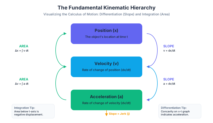
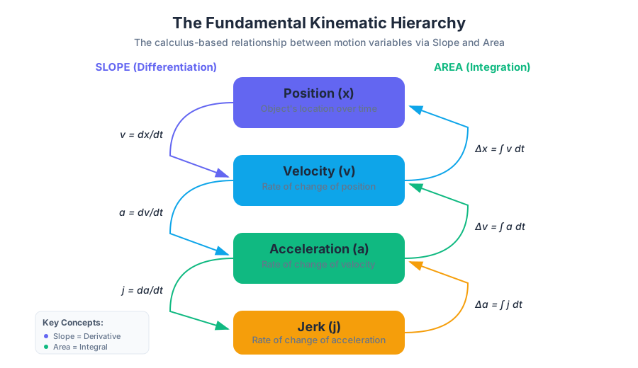
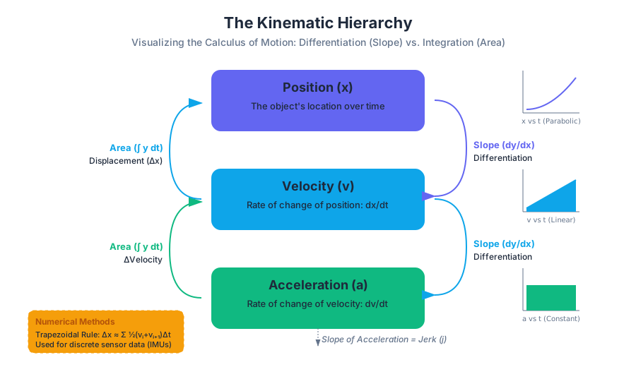
The Fundamental Kinematic Hierarchy
To master graphical analysis, one must understand the hierarchical relationship between position ($x$), velocity ($v$), and acceleration ($a$). These variables are linked through time ($t$) via the operations of differentiation and integration.
| Graph Type | Slope ($dy/dx$) | Area Under Curve ($\int y , dt$) |
|---|---|---|
| Position vs. Time ($x$ vs. $t$) | Velocity ($v$) | No standard physical significance |
| Velocity vs. Time ($v$ vs. $t$) | Acceleration ($a$) | Displacement ($\Delta x$) |
| Acceleration vs. Time ($a$ vs. $t$) | Jerk ($j$) | Change in Velocity ($\Delta v$) |
Position-Time Graphs ($x$ vs. $t$)
The Position-Time Graph is the most intuitive representation of motion. It maps an object's coordinate on a specific axis against the progression of time.
1. Interpreting the Slope
The slope of a position-time graph at any point $t$ is the instantaneous velocity $v(t)$.
Theorem: For a function $x(t)$, the velocity is defined as $v = \lim_{\Delta t \to 0} \frac{\Delta x}{\Delta t} = \frac{dx}{dt}$.
- Linear Slope: Indicates constant velocity. If the line is straight, the object is not accelerating.
- Curvature (Concavity): Indicates acceleration.
- Concave Up (Parabolic): Positive acceleration (velocity is becoming more positive).
- Concave Down: Negative acceleration (velocity is becoming more negative).
- Zero Slope: A horizontal line indicates the object is at rest ($v = 0$).
2. Distance vs. Displacement
A common pitfall in graphical analysis is conflating distance (a scalar) with displacement (a vector).
- Displacement ($\Delta x$): The change in position, calculated as $x_{final} - x_{initial}$. On a graph, this is simply the difference in the y-values between two points.
- Total Distance: The sum of the absolute values of all path segments. If an object moves from $x=0$ to $x=10$ and back to $x=5$, the displacement is $5$, but the distance is $15$.
Velocity-Time Graphs ($v$ vs. $t$)
The Velocity-Time Graph is arguably the most powerful tool in kinematics because it encodes information about position, velocity, and acceleration simultaneously.
1. Slope as Acceleration
The gradient of the $v$ vs. $t$ curve represents the instantaneous acceleration.
- A positive slope means the object is accelerating in the positive direction.
- A negative slope means the object is accelerating in the negative direction (often called deceleration, though this term can be ambiguous if the object is already moving in the negative direction).
2. Area as Displacement
The definite integral of the velocity function with respect to time yields the displacement. $$\Delta x = \int_{t_1}^{t_2} v(t) , dt$$ In a piecewise linear graph (composed of triangles and rectangles), we calculate this area using basic geometry.
| Shape on Graph | Motion Description | Area Calculation |
|---|---|---|
| Rectangle | Constant Velocity | $v \times \Delta t$ |
| Triangle | Constant Acceleration (starting from rest or ending at rest) | $\frac{1}{2} (v_{max} \times \Delta t)$ |
| Trapezoid | Constant Acceleration (between two non-zero velocities) | $\frac{1}{2} (v_1 + v_2) \times \Delta t$ |
3. The "Negative Area" Problem
When the velocity curve dips below the t-axis (negative y-values), the object is moving in the negative direction.
- Net Displacement: Subtract the area below the axis from the area above the axis.
- Total Distance: Add the absolute values of all areas.
Computational Implementation: Discrete Integration
In real-world engineering, such as processing data from an IMU (Inertial Measurement Unit), we do not have continuous functions. Instead, we have discrete data points. We use numerical methods like the Trapezoidal Rule to derive displacement from velocity samples.
import numpy as np

def calculate_kinematics(time_series, velocity_series):
    """
    Computes displacement and acceleration from discrete velocity data.

    Args:
        time_series (np.array): Time stamps in seconds.
        velocity_series (np.array): Velocity samples in m/s.

    Returns:
        displacement (float): Total net displacement.
        acceleration (np.array): Instantaneous acceleration between samples.
    """
    # Calculate acceleration using central differences (slope)
    # a = dv/dt
    acceleration = np.diff(velocity_series) / np.diff(time_series)

    # Calculate displacement using the Trapezoidal Rule (area under curve)
    # dx = integral(v dt)
    displacement = np.trapz(velocity_series, time_series)

    # Calculate total distance (integral of absolute velocity)
    total_distance = np.trapz(np.abs(velocity_series), time_series)

    return displacement, total_distance, acceleration

# Example Data: A car accelerating then braking
t = np.array([0, 2, 4, 6, 8])
v = np.array([0, 10, 20, 10, 0])

disp, dist, acc = calculate_kinematics(t, v)
print(f"Net Displacement: {disp}m, Total Distance: {dist}m")
print(f"Acceleration segments: {acc} m/s^2")
Mathematical Derivation: From Geometry to Equations
The standard kinematic equations for constant acceleration are actually derived from the geometry of a $v$ vs. $t$ graph. Consider an object with initial velocity $v_0$ accelerating at a constant rate $a$ for time $t$.
1. The final velocity (v_f) is the initial velocity plus the change:
   v_f = v_0 + (slope * time)
   v_f = v_0 + at

2. The displacement (delta x) is the area of the trapezoid:
   Area = Area_rectangle + Area_triangle
   delta x = (v_0 * t) + 1/2 * (base * height)
   delta x = v_0 * t + 1/2 * (t * (v_f - v_0))

   Since (v_f - v_0) = at:
   delta x = v_0 * t + 1/2 * a * t^2
Advanced Concept: Curvature and the Second Derivative
In a position-time graph, the "sharpness" of a curve tells us about the magnitude of acceleration. A senior engineer looking at a telemetry log doesn't just look for "up or down"—they look for the Radius of Curvature.
- Inflection Points: A point where the graph changes from concave up to concave down. This represents a local maximum or minimum in velocity and a point where acceleration is zero.
- Jerk ($j$): If the $v$ vs. $t$ graph is itself curved (not a straight line), the acceleration is changing. The rate of change of acceleration is Jerk, which is the slope of the $a$ vs. $t$ graph. High jerk is what humans perceive as "uncomfortable" motion (e.g., a jerky elevator).
Real-World Usage: Embedded Systems Control
In robotics, we often use a PID Controller (Proportional-Integral-Derivative). The "Derivative" term looks at the slope of the error graph (position), while the "Integral" term looks at the area under the error graph.
// C++ snippet for a simple PD controller loop
// Demonstrating the use of slope (derivative) to stabilize motion

float calculate_control_signal(float target_pos, float current_pos, float dt) {
    static float last_error = 0;

    float error = target_pos - current_pos;

    // Proportional term: How far are we?
    float P = Kp * error;

    // Derivative term: How fast are we approaching/leaving? (Slope of error)
    // This acts as a 'damper' to prevent overshoot.
    float D = Kd * (error - last_error) / dt;

    last_error = error;
    return P + D;
}
Common Pitfalls and Misconceptions
1. The "Crossing the Axis" Confusion
On a Velocity-Time graph, crossing the x-axis (from positive to negative velocity) means the object has stopped and reversed direction. It does not necessarily mean the acceleration changed sign. A ball thrown upward has a constant negative acceleration ($g$), but its velocity graph crosses the axis at the peak of its flight.
2. Slope vs. Height
- On an $x$ vs. $t$ graph, the height is where you are; the slope is how fast you're going.
- On a $v$ vs. $t$ graph, the height is how fast you're going; the slope is your acceleration. Users often confuse the two, assuming that because a graph is "high up," the object is moving fast (only true for $v$ vs. $t$).
3. Average vs. Instantaneous
- Average Velocity: The slope of the secant line connecting two points on an $x$ vs. $t$ graph.
- Instantaneous Velocity: The slope of the tangent line at a single point.
| Scenario | $x$ vs. $t$ Shape | $v$ vs. $t$ Shape | $a$ vs. $t$ Shape |
|---|---|---|---|
| Stationary | Horizontal Line | Line on X-axis ($y=0$) | Line on X-axis |
| Constant Velocity | Sloped Straight Line | Horizontal Line | Line on X-axis |
| Constant Acceleration | Parabola | Sloped Straight Line | Horizontal Line |
| Changing Acceleration | Higher-order Curve | Parabola | Sloped Straight Line |
Summary of Problem-Solving Workflow
When faced with a complex motion graph, follow this pipeline:
- Identify the Axes: Is this position, velocity, or acceleration?
- Determine the Goal: Are you looking for a rate of change (slope) or an accumulation (area)?
- Segment the Graph: Break the motion into intervals where the behavior is consistent (e.g., $t=0$ to $t=5$ is constant velocity).
- Calculate Geometric Primitives:
- For slopes: $m = \frac{y_2 - y_1}{x_2 - x_1}$
- For areas: $A = \text{width} \times \text{average height}$
- Check Signs: Is the object moving backward? Is it slowing down? Ensure the signs of your slopes and areas reflect the physical direction.
- Slope of $x-t$ graph: Represents instantaneous velocity ($v$).
- Slope of $v-t$ graph: Represents instantaneous acceleration ($a$).
- Area under $v-t$ graph: Represents displacement ($\Delta x$).
- Area under $a-t$ graph: Represents change in velocity ($\Delta v$).
- Concavity of $x-t$ graph: Indicates the sign of acceleration (Up = Positive, Down = Negative).
- Instantaneous vs Average: Tangent line slope vs. Secant line slope.
- Distance vs Displacement: Total path length (scalar) vs. net change in position (vector).
- If a velocity-time graph is a straight line with a negative slope that crosses the t-axis, what is happening to the object? (Answer: It is slowing down in the positive direction, stops momentarily, then speeds up in the negative direction).
- True or False: An object with a negative velocity and a negative acceleration is slowing down. (Answer: False. It is speeding up in the negative direction).
- How do you find the total distance traveled from a velocity-time graph? (Answer: Sum the absolute values of the areas of all shapes between the curve and the t-axis).
- What does a horizontal line on an acceleration-time graph represent? (Answer: Constant acceleration).
- If the position-time graph is a downward-opening parabola, what can you say about the velocity? (Answer: The velocity is decreasing linearly over time).
Deep Dive Checklist:
- Can you derive the three kinematic equations using only a $v$ vs. $t$ graph?
- Do you understand why the area under a position-time graph has no standard physical meaning? (Units would be $meter \cdot seconds$).
- Can you identify the point of maximum velocity on an $x$ vs. $t$ graph? (Look for the steepest slope).
- Are you comfortable using the Trapezoidal Rule for discrete data sets?
- Can you explain the difference between a "decelerating" object and an object with "negative acceleration"?
Newton's Laws of Motion
Key concepts: Inertia · F=ma · Action-Reaction Pairs · Free-body diagrams · Weight
An exploration of the relationship between forces and motion through Isaac Newton's three fundamental laws.
Newton's Laws of Motion
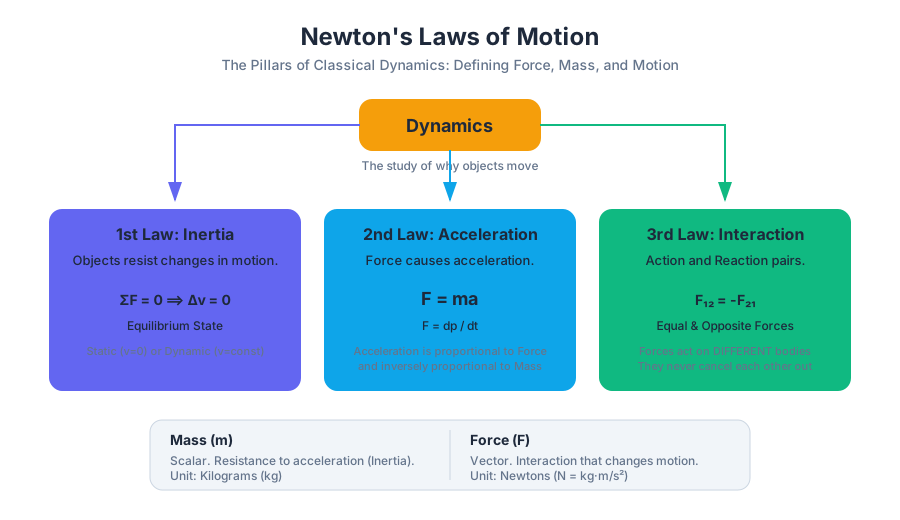
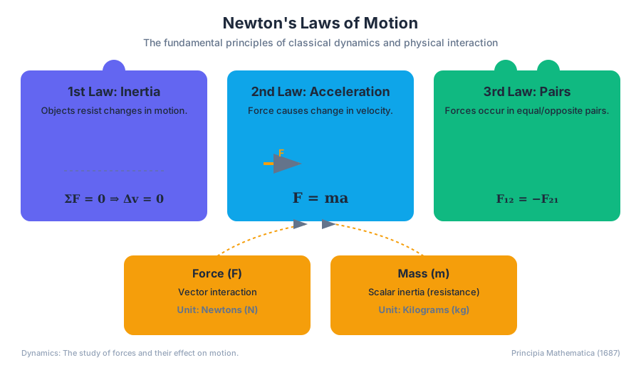
Dynamics is the branch of classical mechanics that addresses the causes of motion. While kinematics describes how objects move (position, velocity, acceleration), dynamics asks why they move. The foundation of this field rests upon three pillars formulated by Sir Isaac Newton in his 1687 masterpiece, Philosophiæ Naturalis Principia Mathematica. These laws are not merely empirical observations; they define the very concepts of mass, force, and momentum within a Galilean reference frame.
The Concept of Force and Mass
Before dissecting the laws, we must establish a rigorous definition of the two primary actors: Force and Mass.
- Force ($\vec{F}$): A vector quantity representing an interaction that, when unopposed, will change the motion of an object. It is measured in Newtons ($N$), where $1 N = 1 kg \cdot m/s^2$.
- Mass ($m$): A scalar quantity representing the intrinsic property of matter that resists acceleration. This is often referred to as Inertial Mass.
| Property | Mass ($m$) | Weight ($W$) | Force ($\vec{F}$) |
|---|---|---|---|
| Definition | Quantity of matter/Inertia | Gravitational pull on mass | Push or pull interaction |
| Type | Scalar | Vector (downward) | Vector |
| Unit | Kilograms ($kg$) | Newtons ($N$) | Newtons ($N$) |
| Variability | Constant regardless of location | Changes with gravity ($g$) | Dependent on interaction |
Newton’s First Law: The Law of Inertia
Theorem: Every object continues in its state of rest, or of uniform motion in a straight line, unless it is compelled to change that state by forces impressed upon it.
The First Law introduces the concept of Inertia—the tendency of an object to resist changes in its state of motion. It essentially defines a special class of reference frames known as Inertial Reference Frames. In these frames, an object with zero net force acting upon it maintains a constant velocity vector ($\vec{v} = \text{constant}$).
The Significance of Equilibrium
When the vector sum of all forces acting on an object is zero ($\sum \vec{F} = 0$), the object is in Translational Equilibrium.
- Static Equilibrium: The object is at rest ($\vec{v} = 0$).
- Dynamic Equilibrium: The object is moving at a constant velocity ($\vec{v} \neq 0, \vec{a} = 0$).
Common Pitfall: The "Force of Motion"
A frequent misconception among students is the "Aristotelian view" that a force is required to keep an object moving. Newton’s First Law explicitly denies this. If a puck slides across an infinite, frictionless ice rink, it requires no force to maintain its velocity. Force is the agent of change, not the agent of existence for motion.
Newton’s Second Law: The Fundamental Equation of Dynamics
Theorem: The acceleration of an object is directly proportional to the net force acting on it and inversely proportional to its mass. The direction of the acceleration is in the direction of the net force.
Mathematically, this is expressed as: $$\sum \vec{F} = m\vec{a}$$
Where $\sum \vec{F}$ (or $\vec{F}_{net}$) is the vector sum of all external forces. This law provides the quantitative link between force and kinematics.
Derivation from Momentum
Newton originally framed the Second Law in terms of Momentum ($\vec{p} = m\vec{v}$). He stated that force is the rate of change of momentum: $$\vec{F} = \frac{d\vec{p}}{dt}$$ If mass is constant: $$\vec{F} = \frac{d(m\vec{v})}{dt} = m\frac{d\vec{v}}{dt} = m\vec{a}$$
Implementation in Computational Physics
In modern engineering, we solve Newton's Second Law using numerical integration. Below is a Python implementation using the Euler-Cromer method to simulate a particle under a constant force (e.g., gravity and drag).
import numpy as np

def simulate_motion(mass, initial_pos, initial_vel, force_func, dt, steps):
    """
    Simulates motion using Newton's Second Law: a = F/m
    """
    # Initialize arrays for position, velocity, and time
    pos = np.zeros((steps, 3))
    vel = np.zeros((steps, 3))
    time = np.linspace(0, steps*dt, steps)

    pos[0] = initial_pos
    vel[0] = initial_vel

    for t in range(1, steps):
        # 1. Calculate Net Force at current state
        net_force = force_func(pos[t-1], vel[t-1])

        # 2. Calculate Acceleration (F = ma => a = F/m)
        accel = net_force / mass

        # 3. Update Velocity (Euler-Cromer for better stability)
        vel[t] = vel[t-1] + accel * dt

        # 4. Update Position
        pos[t] = pos[t-1] + vel[t] * dt

    return time, pos, vel

# Example: Gravity (9.81) and linear air resistance (k=0.1)
def gravity_with_drag(p, v):
    g = np.array([0, -9.81, 0])
    m = 1.0
    k = 0.1
    f_grav = m * g
    f_drag = -k * v
    return f_grav + f_drag

# Usage
t, p, v = simulate_motion(1.0, [0, 100, 0], [10, 0, 0], gravity_with_drag, 0.01, 1000)
Newton’s Third Law: Action and Reaction
Theorem: Whenever one object exerts a force on a second object, the second object exerts an equal and opposite force on the first.
This law is often stated as "For every action, there is an equal and opposite reaction." However, this phrasing leads to the mistake of thinking the forces cancel out. They cannot cancel out because they act on different objects.
Action-Reaction Pairs
An action-reaction pair must satisfy three criteria:
- The forces are equal in magnitude.
- The forces are opposite in direction.
- The forces act on different bodies.
| Situation | Action Force | Reaction Force | Result |
|---|---|---|---|
| Walking | Foot pushes backward on Earth | Earth pushes forward on foot | Person moves forward |
| Rocketry | Rocket pushes gas downward | Gas pushes rocket upward | Rocket accelerates up |
| Gravity | Earth pulls down on Moon | Moon pulls up on Earth | Orbital motion |
| Tug of War | Person A pulls rope | Rope pulls Person A | Tension in rope |
Mathematical Proof of Momentum Conservation
The Third Law is the physical basis for the Law of Conservation of Momentum. If we have two isolated particles interacting:
\begin{aligned}
\vec{F}_{12} &= -\vec{F}_{21} \quad \text{(Newton's 3rd Law)} \\
\frac{d\vec{p}_1}{dt} &= -\frac{d\vec{p}_2}{dt} \quad \text{(Substituting 2nd Law)} \\
\frac{d\vec{p}_1}{dt} + \frac{d\vec{p}_2}{dt} &= 0 \\
\frac{d}{dt}(\vec{p}_1 + \vec{p}_2) &= 0 \\
\vec{p}_{total} &= \text{constant}
\end{aligned}
Free-Body Diagrams (FBDs)
The Free-Body Diagram is the essential analytical tool for applying Newton's Laws. It involves isolating a single body from its environment and representing every external force acting upon it as a vector.
Steps to Construct an FBD
- Isolate the object: Replace the object with a dot (representing the center of mass).
- Identify Field Forces: Draw the weight vector ($W = mg$) pointing straight down.
- Identify Contact Forces: Look for surfaces (Normal force), ropes (Tension), or rough textures (Friction).
- Coordinate System: Choose an axis that aligns with the expected acceleration (e.g., parallel to an inclined plane).
- Decompose Vectors: Resolve any forces not aligned with the axes into $x$ and $y$ components using trigonometry.
Common Forces in FBDs
| Force Name | Symbol | Direction | Magnitude |
|---|---|---|---|
| Weight | $\vec{F}_g$ | Toward center of Earth | $mg$ |
| Normal Force | $\vec{F}_N$ | Perpendicular to surface | Variable (depends on $\sum F_y$) |
| Tension | $\vec{T}$ | Along the string/cable | Variable (equal throughout rope) |
| Friction | $\vec{f}$ | Parallel to surface, opposes motion | $f_s \leq \mu_s F_N$ or $f_k = \mu_k F_N$ |
Weight and Apparent Weight
Weight is the force of gravity acting on an object. Unlike mass, weight is a vector and varies depending on the local gravitational field strength ($g$).
The Normal Force and Apparent Weight
What we "feel" as our weight is actually the Normal Force ($F_N$) exerted by the floor on our feet. In an accelerating frame, such as an elevator, $F_N$ changes, leading to the sensation of being heavier or lighter.
The Elevator Problem Case Study: Consider a person of mass $m$ in an elevator accelerating upward at $a$. Using $\sum F_y = ma$: $$F_N - mg = ma$$ $$F_N = m(g + a)$$
- If $a > 0$ (accelerating up): $F_N > mg$ (You feel heavier).
- If $a < 0$ (accelerating down): $F_N < mg$ (You feel lighter).
- If $a = -g$ (free fall): $F_N = 0$ (Apparent weightlessness).
Real-World Usage: Physics Engine Configuration
In game development or engineering simulations, these laws are codified into "Physics Materials" and "World Settings."
# PhysicsWorldConfig.yaml
world_settings:
  gravity: [0, -9.80665, 0]
  air_density: 1.225 # kg/m^3
  solver_iterations: 10
  allowed_penetration: 0.001

materials:
  steel_on_ice:
    static_friction: 0.03
    kinetic_friction: 0.01
    restitution: 0.5 # Bounciness
  rubber_on_asphalt:
    static_friction: 0.9
    kinetic_friction: 0.8
    restitution: 0.2
Worked Example: The Inclined Plane with Friction
Problem: A block of mass $m = 5 kg$ is placed on a ramp inclined at $\theta = 30^\circ$. The coefficient of kinetic friction is $\mu_k = 0.2$. Calculate the acceleration of the block down the ramp.
1. Identify Forces:
- Gravity ($mg$) acting straight down.
- Normal Force ($F_N$) perpendicular to the ramp.
- Friction ($f_k$) acting up the ramp.
2. Set up Axes: Let $x$ be parallel to the ramp (downward) and $y$ be perpendicular to the ramp.
3. Decompose Gravity:
- $F_{gx} = mg \sin \theta$
- $F_{gy} = mg \cos \theta$
4. Solve for $F_N$ (y-axis equilibrium): $$\sum F_y = F_N - mg \cos \theta = 0 \implies F_N = mg \cos \theta$$
5. Solve for $a$ (x-axis dynamics): $$\sum F_x = mg \sin \theta - f_k = ma$$ Since $f_k = \mu_k F_N = \mu_k mg \cos \theta$: $$mg \sin \theta - \mu_k mg \cos \theta = ma$$ $$a = g(\sin \theta - \mu_k \cos \theta)$$
6. Plug in values: $$a = 9.8 (\sin 30^\circ - 0.2 \cos 30^\circ)$$ $$a = 9.8 (0.5 - 0.2 \times 0.866) = 9.8 (0.5 - 0.1732) = 3.20 \text{ m/s}^2$$
Advanced Extensions: Non-Inertial Frames
When we observe motion from an accelerating frame (like a turning car or a rotating space station), Newton's Laws appear to fail unless we introduce Fictitious Forces (or Inertial Forces).
- Centrifugal Force: The outward "force" felt in a rotating frame.
- Coriolis Force: The force that deflects moving objects in a rotating frame, crucial for atmospheric science.
In these frames, the Second Law is modified to: $$\vec{F}{net} + \vec{F}{fictitious} = m\vec{a}_{observed}$$
This highlights that Newton's Laws are not just equations, but a definition of the geometry of the space in which we measure motion.

Two-Dimensional Motion and Vectors
Key concepts: Vector Analysis · Projectile Motion · Inclined Planes · Static and Kinetic Friction
Expanding motion analysis to two dimensions using vector components, projectile motion, and friction.
Two-Dimensional Motion and Vectors
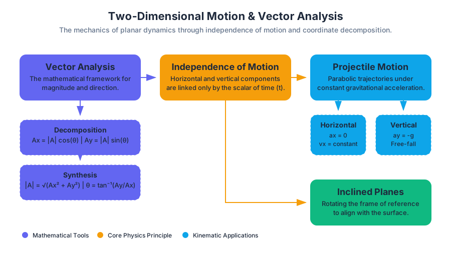
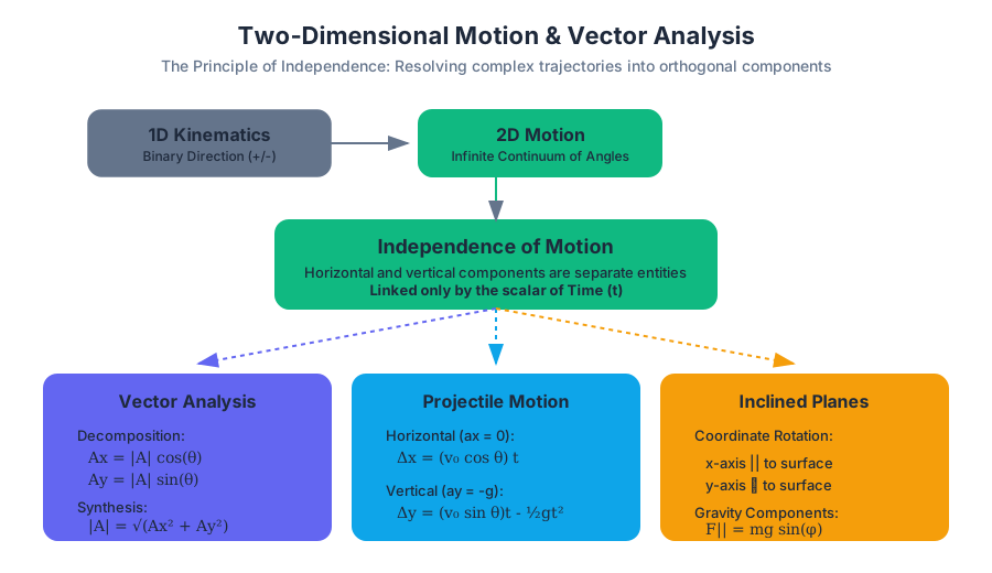
The transition from one-dimensional kinematics to two-dimensional motion represents a fundamental leap in classical mechanics. In a 1D world, direction is binary (positive or negative). In 2D, we must contend with an infinite continuum of directions, requiring a robust mathematical framework to maintain precision. This section explores the mechanics of objects moving through a plane, governed by the principle of independence of motion, where horizontal and vertical components are treated as separate yet simultaneous entities linked only by the scalar of time.
Vector Analysis: The Language of 2D Space
At the heart of multidimensional physics lies Vector Analysis. Unlike scalars (such as mass or temperature), which only possess magnitude, vectors (such as displacement, velocity, and force) require both magnitude and direction. To manipulate these effectively, we employ orthonormal decomposition—breaking a single vector into its constituent $x$ (horizontal) and $y$ (vertical) components.
Vector Decomposition and Synthesis
Any vector $\vec{A}$ at an angle $\theta$ relative to the positive x-axis can be resolved into components using basic trigonometry:
- $A_x = |\vec{A}| \cos(\theta)$
- $A_y = |\vec{A}| \sin(\theta)$
Conversely, the magnitude and direction can be recovered from the components:
- $|\vec{A}| = \sqrt{A_x^2 + A_y^2}$
- $\theta = \tan^{-1}\left(\frac{A_y}{A_x}\right)$
| Operation | Mathematical Definition | Physical Interpretation |
|---|---|---|
| Addition | $\vec{R} = (A_x + B_x)\hat{i} + (A_y + B_y)\hat{j}$ | Finding the net effect of multiple forces or displacements. |
| Scalar Multi. | $k\vec{A} = (kA_x)\hat{i} + (kA_y)\hat{j}$ | Scaling a vector (e.g., $F = ma$ scales acceleration by mass). |
| Dot Product | $\vec{A} \cdot \vec{B} = \vert \vec{A}\vert \vert \vec{B}\vert \cos(\phi)$ | Calculating work done or projecting one vector onto another. |
| Unit Vector | $\hat{u} = \frac{\vec{A}}{\vert \vec{A}\vert }$ | Defining a pure direction with a magnitude of 1. |
The Principle of Superposition: The net response of a system at a given place and time caused by two or more stimuli is the sum of the responses that would have been caused by each stimulus individually. In 2D motion, this means we can solve the $x$-dynamics and $y$-dynamics independently.
import numpy as np

class Vector2D:
    """
    Low-level implementation of 2D Vector operations for physics simulations.
    Uses NumPy for high-performance floating-point arithmetic.
    """
    def __init__(self, x, y):
        self.components = np.array([float(x), float(y)])

    @property
    def x(self): return self.components[0]

    @property
    def y(self): return self.components[1]

    def magnitude(self):
        return np.linalg.norm(self.components)

    def angle(self, degrees=False):
        angle_rad = np.arctan2(self.y, self.x)
        return np.degrees(angle_rad) if degrees else angle_rad

    def __add__(self, other):
        res = self.components + other.components
        return Vector2D(res[0], res[1])

    def dot(self, other):
        return np.dot(self.components, other.components)

    def __repr__(self):
        return f"Vector2D(x={self.x:.2f}, y={self.y:.2f}, mag={self.magnitude():.2f})"

# Example: Resolving a force of 50N at 30 degrees
force_mag = 50
angle = np.radians(30)
f_vec = Vector2D(force_mag * np.cos(angle), force_mag * np.sin(angle))
print(f_vec)
Projectile Motion: Dynamics under Gravity
Projectile Motion is the motion of an object thrown or projected into the air, subject only to the acceleration of gravity. In an idealized vacuum, the horizontal component of velocity remains constant because no horizontal forces act upon the object (ignoring air resistance). The vertical component, however, is in a state of constant free-fall acceleration.
The Kinematic Framework
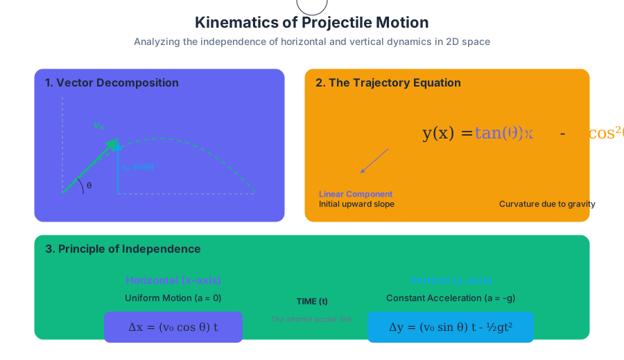
To solve projectile problems, we split the motion into two sets of equations. Let $v_0$ be the initial velocity and $\theta$ be the launch angle.
Horizontal ($x$):
- $a_x = 0$
- $v_x = v_0 \cos(\theta)$
- $\Delta x = (v_0 \cos(\theta))t$
Vertical ($y$):
- $a_y = -g$ (where $g \approx 9.81 , \text{m/s}^2$)
- $v_y = v_0 \sin(\theta) - gt$
- $\Delta y = (v_0 \sin(\theta))t - \frac{1}{2}gt^2$
Derivation: The Trajectory Equation
By isolating $t$ in the horizontal equation ($t = \frac{x}{v_0 \cos(\theta)}$) and substituting it into the vertical displacement equation, we derive the path of the projectile:
y(x) = \tan(\theta)x - \frac{g}{2v_0^2 \cos^2(\theta)}x^2
This is the equation of a parabola. This mathematical reality explains why every thrown ball, launched missile, or leaping athlete follows a parabolic arc.
| Parameter | Impact on Trajectory |
|---|---|
| Launch Angle ($\theta$) | Determines the balance between "hang time" and horizontal reach. $45^\circ$ yields max range. |
| Initial Velocity ($v_0$) | Scales the entire trajectory; range increases with the square of $v_0$. |
| Gravity ($g$) | Inversely proportional to range and height; lower gravity (Moon) leads to longer arcs. |
| Initial Height ($h_0$) | Shifts the parabola upward, increasing time in air and horizontal range. |
Inclined Planes: Rotating the Frame of Reference
When an object moves along a slope, gravity no longer acts purely along the axis of motion. To simplify the mathematics, we perform a coordinate rotation. Instead of using standard horizontal and vertical axes, we align the $x$-axis parallel to the surface of the incline and the $y$-axis perpendicular to it.
Force Decomposition on a Slope
Consider an object of mass $m$ on a plane inclined at angle $\phi$. Gravity ($F_g = mg$) acts straight down. We resolve $F_g$ into:
- Parallel Component ($F_{g\parallel}$): $mg \sin(\phi)$. This is the force pulling the object down the slope.
- Perpendicular Component ($F_{g\perp}$): $mg \cos(\phi)$. This component presses the object into the surface and is countered by the Normal Force ($F_N$).
The Normal Force ($F_N$): On an inclined plane with no other vertical forces, $F_N = mg \cos(\phi)$. As the angle $\phi$ increases, $\cos(\phi)$ decreases, meaning the surface "feels" less weight from the object.
Acceleration on a Frictionless Incline
Using Newton’s Second Law ($F = ma$): $mg \sin(\phi) = ma$ $a = g \sin(\phi)$
This elegant result shows that the acceleration of an object down a frictionless ramp is independent of its mass and depends solely on the tilt of the ramp.
Static and Kinetic Friction
Friction is the resistive force that opposes the relative motion (or intended motion) of two surfaces in contact. It is a complex electromagnetic interaction between surface atoms, but for classical mechanics, we use the Coulomb Friction Model.
Static Friction ($f_s$)
Static friction acts on objects that are not yet moving. It is a "responsive" force—it only pushes back as hard as you push it, up to a certain threshold.
- Formula: $f_s \leq \mu_s F_N$
- $\mu_s$: The coefficient of static friction.
- Threshold: The moment $F_{applied} > \mu_s F_N$, the object breaks free and begins to move.
Kinetic Friction ($f_k$)
Once the object is in motion, the bonds between surfaces cannot fully reform, leading to a lower resistive force.
- Formula: $f_k = \mu_k F_N$
- $\mu_k$: The coefficient of kinetic friction.
- Rule: Generally, $\mu_k < \mu_s$. This is why it is harder to start sliding a heavy box than it is to keep it moving.
| Feature | Static Friction ($f_s$) | Kinetic Friction ($f_k$) |
|---|---|---|
| State of Motion | Stationary | Moving |
| Magnitude | Variable (0 up to $f_{s,max}$) | Constant (mostly) |
| Direction | Opposes potential motion | Opposes actual velocity vector |
| Coefficient | Higher ($\mu_s$) | Lower ($\mu_k$) |
Worked Example: The Angle of Repose
What is the maximum angle $\phi$ an incline can have before a block starts to slide? At the verge of sliding, the parallel gravitational force equals the maximum static friction: $mg \sin(\phi) = \mu_s (mg \cos(\phi))$ $\frac{\sin(\phi)}{\cos(\phi)} = \mu_s$ $\tan(\phi) = \mu_s$
The angle $\phi = \tan^{-1}(\mu_s)$ is known as the Angle of Repose.
# Example: Physics Engine Configuration for Friction Materials
materials:
  rubber_on_asphalt:
    static_friction: 0.9
    kinetic_friction: 0.67
    restitution: 0.5 # Bounciness
  ice_on_steel:
    static_friction: 0.03
    kinetic_friction: 0.02
    restitution: 0.1
  wood_on_wood:
    static_friction: 0.4
    kinetic_friction: 0.2
Common Pitfalls and Misconceptions
- The "Gravity acts on the x-axis" Error: Students often forget that in projectile motion, $a_x$ is strictly zero (in the absence of air resistance). There is no force pushing the projectile forward after it leaves the launcher.
- Normal Force Misconception: $F_N$ is not always equal to $mg$. On an incline, it is $mg \cos(\phi)$. If you are in an elevator or being pulled at an angle, $F_N$ changes. Always use a Free Body Diagram (FBD) to sum forces in the perpendicular direction.
- Friction Direction: Friction does not always oppose the "direction of the object." It opposes the relative motion between surfaces. In the case of walking, static friction actually points forward, as it prevents your foot from sliding backward, thus propelling you.
- The $\mu$ limit: The coefficients of friction $\mu$ are empirical approximations. In extreme cases (high speeds, high pressures, or very smooth surfaces like silicon wafers), the linear $f = \mu F_N$ model breaks down.
Summary of 2D Dynamics Pipeline
To solve any complex 2D motion problem (e.g., a block sliding down a ramp and then becoming a projectile), follow this engineering pipeline:
- Identify the Phases: Break the motion into distinct segments (e.g., Phase 1: Incline, Phase 2: Free fall).
- Establish Coordinate Systems: Rotate axes for inclines; use standard Cartesian for projectiles.
- Free Body Diagrams: Draw all forces ($F_g, F_N, f, F_{app}$).
- Component Resolution: Use $\sin$ and $\cos$ to align all forces/velocities with your chosen axes.
- Apply Newton's Second Law: $\sum F_x = ma_x$ and $\sum F_y = ma_y$.
- Link via Time: Use kinematic equations to solve for unknowns, using $t$ as the bridge between $x$ and $y$ components.
Core Equations Reference
- Range of Projectile: $R = \frac{v_0^2 \sin(2\theta)}{g}$
- Max Height of Projectile: $H = \frac{v_0^2 \sin^2(\theta)}{2g}$
- Acceleration on Incline with Friction: $a = g(\sin(\phi) - \mu_k \cos(\phi))$
- Vector Magnitude: $v = \sqrt{v_x^2 + v_y^2}$
Work, Energy, and Power
Key concepts: Work-Energy Theorem · Kinetic Energy · Potential Energy · Conservation of Energy · Power
Defining work and energy, and exploring the law of conservation of energy in physical systems.
Work, Energy, and Power
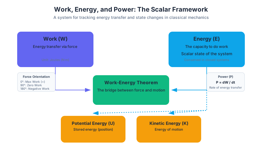
In classical mechanics, we often begin by analyzing motion through the lens of Newton’s Laws. However, as systems grow in complexity—involving varying forces or intricate paths—the vector-based approach of $\vec{F} = m\vec{a}$ becomes computationally taxing. The study of Work, Energy, and Power provides a scalar alternative: a powerful "accounting system" for the universe. By focusing on the state of a system rather than the instantaneous forces acting upon it, we can solve complex trajectories and predict final states with remarkable precision.
The Concept of Work
In physics, Work ($W$) is not merely effort; it is the measure of energy transfer that occurs when a force is applied over a displacement. If a force has no component in the direction of motion, no work is performed on the object, regardless of how much "effort" is expended.
What it is
Mathematically, for a constant force, work is the dot product of the force vector $\vec{F}$ and the displacement vector $\vec{d}$:
$$W = \vec{F} \cdot \vec{d} = Fd \cos \theta$$
Where $\theta$ is the angle between the force and the displacement. In a more general sense, where force varies along a path, work is defined as a line integral:
$$W = \int_{C} \vec{F} \cdot d\vec{r}$$
Why it matters
Work bridges the gap between dynamics (forces) and kinematics (motion). It quantifies how an external influence changes the energy state of an object. Without the concept of work, we would have no formal way to describe how a battery moves a car or how a star's gravity pulls a planet into a tighter orbit.
Mechanics and Scenarios
The value of work depends entirely on the orientation of the force relative to the displacement.
| Scenario | Angle ($\theta$) | Work Done ($W$) | Physical Meaning |
|---|---|---|---|
| Aligned | $0^\circ$ | $Fd$ (Maximum Positive) | Force adds energy to the system (e.g., pushing a sled). |
| Opposed | $180^\circ$ | $-Fd$ (Maximum Negative) | Force removes energy (e.g., kinetic friction slowing a block). |
| Perpendicular | $90^\circ$ | $0$ | Force changes direction but not speed (e.g., centripetal force). |
| Obtuse | $90^\circ < \theta \leq 180^\circ$ | Negative | The force hinders the motion. |
Concrete Example: Numerical Integration of Work
In real-world engineering, forces are rarely constant. Consider a variable force $F(x) = kx^2$ acting on a particle. To find the work done from $x=0$ to $x=5$, we must integrate.
/*
 * Low-level implementation: Numerical Integration of Work
 * Using the Trapezoidal Rule to calculate work done by a variable force.
 */

#include <stdio.h>

double variable_force(double x) {
    // Example: F(x) = 10 * x^2 (a non-linear spring or resistance)
    return 10.0 * (x * x);
}

double calculate_work(double start, double end, int intervals) {
    double dx = (end - start) / intervals;
    double total_work = 0.0;

    for (int i = 0; i < intervals; i++) {
        double x1 = start + i * dx;
        double x2 = start + (i + 1) * dx;
        // Trapezoidal area: (f(x1) + f(x2)) / 2 * dx
        total_work += (variable_force(x1) + variable_force(x2)) / 2.0 * dx;
    }
    return total_work;
}

int main() {
    double work = calculate_work(0.0, 5.0, 1000);
    printf("Total Work Done: %.4f Joules\n", work);
    return 0;
}
Kinetic Energy and the Work-Energy Theorem
Kinetic Energy ($K$ or $KE$) represents the energy an object possesses due to its motion. It is a scalar quantity, always non-negative, and depends on the square of the velocity.
The Derivation
We can derive the expression for Kinetic Energy using Newton's Second Law and kinematic equations. For a constant force $F$ acting on a mass $m$ over distance $d$:
- $W = Fd$
- From $F = ma$, we get $W = mad$
- From kinematics, $v_f^2 = v_i^2 + 2ad$, which implies $ad = \frac{v_f^2 - v_i^2}{2}$
- Substituting $ad$ into the work equation: $W = m(\frac{v_f^2 - v_i^2}{2})$
- $W = \frac{1}{2}mv_f^2 - \frac{1}{2}mv_i^2$
The Work-Energy Theorem: The net work done by all forces acting on a particle equals the change in the particle's kinetic energy. $$W_{net} = \Delta K = K_f - K_i$$
Why it Matters
This theorem is a shortcut. If you know the initial speed of a car and the work done by the brakes (friction), you can calculate the final speed without ever calculating the time elapsed or the instantaneous acceleration.
Common Pitfalls
- Velocity is Squared: Doubling the speed of a vehicle quadruples its kinetic energy ($2^2 = 4$). This is why high-speed crashes are significantly more lethal than low-speed ones.
- Frame of Reference: While energy is a scalar, velocity is relative. Kinetic energy depends on the observer's frame of reference.
Potential Energy: Stored Capability
Potential Energy ($U$ or $PE$) is the energy stored within a system due to the configuration or position of its parts. It represents the "potential" to do work.
Gravitational Potential Energy ($U_g$)
Near the Earth's surface, the gravitational potential energy is proportional to the height $h$ relative to a chosen reference point (datum): $$U_g = mgh$$
Elastic Potential Energy ($U_s$)
When a spring is compressed or stretched, it stores energy. This follows Hooke's Law ($F = -kx$), where $k$ is the spring constant.
\begin{aligned}
W_s &= \int_{0}^{x} F_{ext} \, dx \\
W_s &= \int_{0}^{x} kx \, dx \\
U_s &= \frac{1}{2}kx^2
\end{aligned}
Conservative vs. Non-Conservative Forces
Potential energy can only be defined for conservative forces.
| Feature | Conservative Forces (e.g., Gravity, Elastic) | Non-Conservative Forces (e.g., Friction, Air Drag) |
|---|---|---|
| Path Dependency | Independent of path taken. | Dependent on path taken. |
| Work on Closed Loop | Zero. | Non-zero (usually negative). |
| Energy Recovery | Energy can be fully recovered. | Energy is dissipated as heat/sound. |
| Potential Energy | Can be defined ($U$). | Cannot be defined. |
Conservation of Energy
The Law of Conservation of Energy states that the total energy of an isolated system remains constant. Energy is neither created nor destroyed; it only transforms from one form to another.
Mechanical Energy
In systems where only conservative forces act, the Total Mechanical Energy ($E_{mech}$) is conserved: $$E_i = E_f \implies K_i + U_i = K_f + U_f$$
The General Energy Equation
In the presence of non-conservative forces like friction ($W_{fric}$), the equation expands: $$K_i + U_i + W_{other} = K_f + U_f$$ Here, $W_{other}$ is usually negative, representing energy leaving the mechanical system (often turning into thermal energy).
Worked Example: The Roller Coaster
A 500 kg roller coaster car starts from rest at the top of a 40m hill. How fast is it going at the bottom of the hill (assume no friction)?
- Initial State: $v_i = 0 \implies K_i = 0$. $h_i = 40m \implies U_i = mgh_i$.
- Final State: $h_f = 0 \implies U_f = 0$. $K_f = \frac{1}{2}mv_f^2$.
- Conservation: $mgh_i = \frac{1}{2}mv_f^2$
- Solve for $v_f$: $v_f = \sqrt{2gh_i} = \sqrt{2 \cdot 9.8 \cdot 40} \approx 28 \text{ m/s}$.
Note that the mass $m$ cancels out—a heavy car and a light car will reach the bottom at the same speed (ignoring air resistance).
Power: The Rate of Energy Transfer
Power ($P$) is the rate at which work is done or energy is transformed. In engineering, power is often more critical than the total energy; a powerful engine isn't just one that can move a heavy load, but one that can move it quickly.
Mathematical Definition
Average power is work divided by time: $$P_{avg} = \frac{W}{\Delta t}$$
Instantaneous power is the derivative of work with respect to time: $$P = \frac{dW}{dt} = \vec{F} \cdot \vec{v}$$
Units and Conversions
The SI unit of power is the Watt (W), defined as 1 Joule per second.
| Unit | Equivalent in Watts | Context |
|---|---|---|
| 1 Watt (W) | $1 \text{ J/s}$ | Electronics, light bulbs. |
| 1 Kilowatt (kW) | $1,000 \text{ W}$ | Household appliances, small motors. |
| 1 Horsepower (hp) | $\approx 746 \text{ W}$ | Automotive and industrial engines. |
| 1 Megawatt (MW) | $10^6 \text{ W}$ | Power plants, locomotives. |
Real-World Usage Example: Performance Analysis
Engineers use power-to-weight ratios to determine the acceleration capabilities of vehicles.
import numpy as np

def analyze_vehicle_power(velocity_m_s, force_n, mass_kg):
    """
    Calculates instantaneous power and acceleration.
    """
    # P = F * v
    power_watts = force_n * velocity_m_s
    power_hp = power_watts / 745.7

    # F = m * a -> a = F / m
    acceleration = force_n / mass_kg

    return {
        "Power (W)": round(power_watts, 2),
        "Power (hp)": round(power_hp, 2),
        "Acceleration (m/s^2)": round(acceleration, 2)
    }

# Example: A 1500kg car moving at 30 m/s (approx 67 mph)
# with a driving force of 4000 N.
stats = analyze_vehicle_power(30, 4000, 1500)
print(f"Vehicle Stats: {stats}")
Simple Machines and Mechanical Advantage
Simple machines (levers, pulleys, inclined planes) do not reduce the amount of work required to perform a task. Instead, they allow us to perform that work by applying a smaller force over a larger distance.
Efficiency
In the real world, no machine is 100% efficient due to friction. $$\text{Efficiency} (\eta) = \frac{W_{out}}{W_{in}} \times 100%$$
Mechanical Advantage (MA)
- Ideal Mechanical Advantage (IMA): The ratio of distances ($d_{in} / d_{out}$).
- Actual Mechanical Advantage (AMA): The ratio of forces ($F_{out} / F_{in}$).
| Machine | IMA Formula | How it works |
|---|---|---|
| Lever | $L_{effort} / L_{resistance}$ | Trades distance from fulcrum for force. |
| Inclined Plane | $L / h$ | Spreads the lift over a longer horizontal distance. |
| Pulley System | Number of rope segments | Distributes weight across multiple tension points. |
Summary of Pitfalls and Edge Cases
- The "Holding a Box" Fallacy: If you hold a 50kg box perfectly still, you are doing zero physical work ($d=0$), even though your muscles are consuming chemical energy and you feel tired.
- Centripetal Force: A planet orbiting a star in a perfect circle has a force (gravity) acting on it, but because the force is always perpendicular to the velocity, the work done by gravity is zero, and the kinetic energy remains constant.
- Negative Work: Friction always does negative work because it opposes motion. This energy isn't "lost" from the universe; it is converted into internal (thermal) energy of the surfaces.

Linear Momentum and Collisions
Key concepts: Linear Momentum · Impulse · Conservation of Momentum · Elastic vs. Inelastic Collisions · Center of Mass
The study of momentum, impulse, and the behavior of objects during elastic and inelastic collisions.
Linear Momentum and Collisions
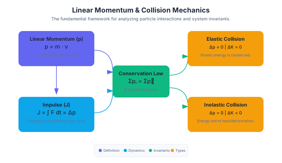
Linear momentum is the fundamental metric of an object's motion, encapsulating both its inertia and its velocity. While Newton’s Second Law is often introduced as $F = ma$, Newton’s original formulation was more profound: force is the rate of change of momentum. This section explores the mechanics of how objects interact, the invariants that govern those interactions, and the mathematical frameworks used to predict the outcomes of everything from subatomic scattering to galactic mergers.
Linear Momentum: The Quantity of Motion
Linear momentum, denoted by the vector p, is defined as the product of an object's mass and its velocity. It is a vector quantity, meaning it possesses both magnitude and direction.
Definition: The linear momentum $\vec{p}$ of a particle of mass $m$ moving with velocity $\vec{v}$ is defined as: $$\vec{p} = m\vec{v}$$ The SI unit of momentum is the kilogram-meter per second ($kg \cdot m/s$).
Why Momentum Matters
While kinetic energy ($K = \frac{1}{2}mv^2$) describes the scalar "scalar energy" of motion, momentum describes the "directed persistence" of motion. Because momentum is proportional to $\vec{v}$ (rather than $v^2$), it is conserved in a way that kinetic energy is not. In any closed system, the total vector momentum remains constant, regardless of the complexity of the internal interactions.
Relativistic Considerations
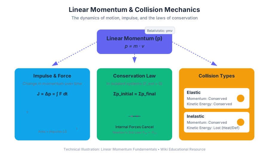
At velocities approaching the speed of light $c$, the classical definition fails. Senior engineers working with particle accelerators or high-energy physics must use the relativistic momentum: $$\vec{p} = \gamma m \vec{v} = \frac{m\vec{v}}{\sqrt{1 - \frac{v^2}{c^2}}}$$
| Parameter | Symbol | Type | Description |
|---|---|---|---|
| Mass | $m$ | Scalar | The inertial resistance to acceleration (kg). |
| Velocity | $\vec{v}$ | Vector | The rate of change of position (m/s). |
| Momentum | $\vec{p}$ | Vector | The product of mass and velocity ($kg \cdot m/s$). |
| Force | $\vec{F}$ | Vector | The time-derivative of momentum ($dp/dt$). |
Impulse and the Impulse-Momentum Theorem
When a force acts on an object over a duration of time, it changes the object's momentum. This change is defined as Impulse ($\vec{J}$).
The Derivation
Starting from Newton's Second Law in its differential form: $$\vec{F} = \frac{d\vec{p}}{dt}$$ Integrating both sides with respect to time from $t_1$ to $t_2$: $$\int_{t_1}^{t_2} \vec{F} dt = \int_{p_1}^{p_2} d\vec{p} = \vec{p}_2 - \vec{p}_1 = \Delta \vec{p}$$
The integral of force over time is the Impulse: $$\vec{J} = \int \vec{F} dt = \Delta \vec{p}$$
Force-Time Graphs
In real-world collisions (like a bat hitting a ball), the force is not constant. It spikes rapidly and then decays. The impulse is the area under the Force-vs-Time curve. For practical engineering, we often use the Average Force ($F_{avg}$): $$\vec{J} = \vec{F}_{avg} \Delta t$$
Implementation: Numerical Integration of Impulse
In physics engines or telemetry analysis, we often have discrete force samples. We can calculate the resulting change in velocity using the trapezoidal rule.
/*
 * Low-level implementation of Impulse-Momentum integration.
 * Calculates the final velocity of a body given a series of force samples.
 */
#include <stdio.h>

typedef struct {
    double mass;
    double velocity;
} RigidBody;

double calculate_final_velocity(RigidBody *body, double force_samples[], double dt, int n) {
    double impulse = 0.0;

    // Numerical integration using the Trapezoidal Rule
    for (int i = 0; i < n - 1; i++) {
        impulse += 0.5 * (force_samples[i] + force_samples[i+1]) * dt;
    }

    // Delta V = Impulse / Mass
    double delta_v = impulse / body->mass;
    body->velocity += delta_v;

    return body->velocity;
}

int main() {
    RigidBody car = {1500.0, 0.0}; // 1500kg car at rest
    double forces[] = {0, 5000, 10000, 8000, 2000, 0}; // Force in Newtons
    double dt = 0.01; // 10ms sampling rate

    double v_final = calculate_final_velocity(&car, forces, dt, 6);
    printf("Final Velocity: %.2f m/s\n", v_final);
    return 0;
}
Conservation of Momentum
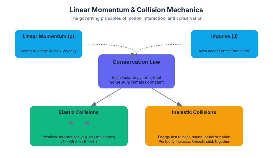
The Law of Conservation of Momentum states that if the net external force acting on a system is zero, the total momentum of the system remains constant.
The Principle: $$\sum \vec{p}{initial} = \sum \vec{p}{final}$$ This holds true even if kinetic energy is lost, as long as no external forces (like friction or gravity) interfere with the system during the interaction.
Internal vs. External Forces
- Internal Forces: Forces between objects within the system (e.g., two billiard balls hitting each other). These occur in action-reaction pairs ($F_{12} = -F_{21}$) and cancel out in the total momentum sum.
- External Forces: Forces from outside the system (e.g., gravity, friction). These are the only forces capable of changing the system's total momentum.
| System Type | External Forces | Momentum | Energy |
|---|---|---|---|
| Isolated | Zero | Conserved | Conserved (Total) |
| Closed | Non-zero | Not Conserved | Conserved (Total) |
| Open | Non-zero | Not Conserved | Not Conserved |
Elastic vs. Inelastic Collisions
Collisions are categorized based on whether Kinetic Energy ($K$) is conserved alongside momentum.
1. Elastic Collisions
In a perfectly elastic collision, both momentum and kinetic energy are conserved. These are common in subatomic particles or idealized gas molecules.
- Momentum: $m_1 v_{1i} + m_2 v_{2i} = m_1 v_{1f} + m_2 v_{2f}$
- Kinetic Energy: $\frac{1}{2}m_1 v_{1i}^2 + \frac{1}{2}m_2 v_{2i}^2 = \frac{1}{2}m_1 v_{1f}^2 + \frac{1}{2}m_2 v_{2f}^2$
The Relative Velocity Theorem: In a 1D elastic collision, the relative speed of approach equals the relative speed of recession: $$v_{1i} - v_{2i} = -(v_{1f} - v_{2f})$$
2. Inelastic Collisions
In an inelastic collision, momentum is conserved, but some kinetic energy is converted into other forms (heat, sound, deformation).
- Perfectly Inelastic: The objects stick together after impact ($v_{1f} = v_{2f} = V$). This results in the maximum possible loss of kinetic energy.
- Partially Inelastic: The objects bounce, but with reduced speed.
The Coefficient of Restitution ($e$)
The "bounciness" of a collision is quantified by $e$: $$e = \frac{|v_{2f} - v_{1f}|}{|v_{1i} - v_{2i}|}$$
- $e = 1$: Perfectly Elastic
- $e = 0$: Perfectly Inelastic
- $0 < e < 1$: Real-world Inelastic
/* Mathematical Derivation of 1D Elastic Collision Final Velocities */

Given: m1, m2, v1i, v2i
Solve for v1f, v2f:

Step 1: Conservation of Momentum
m1*v1i + m2*v2i = m1*v1f + m2*v2f

Step 2: Relative Velocity Theorem (derived from KE conservation)
v1i - v2i = v2f - v1f  => v2f = v1f + v1i - v2i

Step 3: Substitute (2) into (1)
m1*v1i + m2*v2i = m1*v1f + m2*(v1f + v1i - v2i)

Resulting Formulas:
v1f = [ (m1 - m2)/(m1 + m2) ] * v1i + [ (2*m2)/(m1 + m2) ] * v2i
v2f = [ (2*m1)/(m1 + m2) ] * v1i + [ (m2 - m1)/(m1 + m2) ] * v2i
Center of Mass (COM)
The Center of Mass is the unique point where the weighted relative position of the distributed mass sums to zero. It is the point that moves as if all the system's mass were concentrated there and all external forces were applied there.
Mathematical Definition
For a system of $n$ particles: $$\vec{R}{cm} = \frac{1}{M} \sum{i=1}^{n} m_i \vec{r}i$$ Where $M = \sum m_i$. For continuous objects, we use integration: $$\vec{R}{cm} = \frac{1}{M} \int \vec{r} dm$$
Motion of the Center of Mass
The velocity of the center of mass ($\vec{V}{cm}$) is directly related to the total momentum of the system ($\vec{P}{tot}$): $$\vec{P}{tot} = M \vec{V}{cm}$$ If the net external force is zero, $\vec{V}_{cm}$ is constant. This leads to a powerful insight: Internal explosions or collisions do not change the trajectory of the center of mass. If a projectile explodes in mid-air, the center of mass of the fragments continues to follow the original parabolic path (ignoring air resistance).
| Geometry | Center of Mass Location |
|---|---|
| Uniform Rod | Geometric center ($L/2$). |
| Solid Sphere | Geometric center. |
| Right Triangle | $1/3$ height from the base, $1/3$ width from the vertical. |
| Semicircle (Wire) | $2r/\pi$ from the diameter. |
| Semicircle (Disk) | $4r/3\pi$ from the diameter. |
Example: Calculating COM for a Point Cloud
In robotics or computer vision, we often need to find the centroid of a set of detected points (masses).
import numpy as np

def calculate_center_of_mass(points, masses):
    """
    Calculates the COM of a system of particles.
    :param points: Nx3 array of (x, y, z) coordinates
    :param masses: N-length array of mass values
    :return: 1x3 array representing the COM coordinate
    """
    total_mass = np.sum(masses)
    if total_mass == 0:
        raise ValueError("Total mass cannot be zero.")

    # Weighted sum of positions: sum(m_i * r_i)
    weighted_positions = np.sum(points * masses[:, np.newaxis], axis=0)

    return weighted_positions / total_mass

# Real-world usage: A drone with 4 motors
motor_positions = np.array([
    [0.2, 0.2, 0],   # Motor 1
    [-0.2, 0.2, 0],  # Motor 2
    [-0.2, -0.2, 0], # Motor 3
    [0.2, -0.2, 0]   # Motor 4
])
motor_masses = np.array([0.1, 0.1, 0.1, 0.1]) # 100g each
frame_mass = 0.5
frame_pos = np.array([0, 0, 0.05])

all_points = np.vstack([motor_positions, frame_pos])
all_masses = np.append(motor_masses, frame_mass)

com = calculate_center_of_mass(all_points, all_masses)
print(f"System Center of Mass: {com}")
Multi-Dimensional Collisions
In two or three dimensions, momentum conservation must be applied independently to each axis ($x, y, z$).
Strategy for 2D Collisions
- Decompose initial velocities into $v_x$ and $v_y$ components using trigonometry.
- Apply Conservation for each axis:
- $\sum p_{ix} = \sum p_{fx}$
- $\sum p_{iy} = \sum p_{fy}$
- Solve the resulting system of equations.
- Reconstruct the final velocity vectors using the Pythagorean theorem and $\arctan(v_y/v_x)$.
Common Pitfall: Glancing Collisions
In a glancing elastic collision between two identical masses ($m_1 = m_2$) where one is initially at rest, the two masses will always move away at a 90-degree angle to each other. This is a favorite concept in physics exams and billiards.
Summary of Collision Dynamics
| Feature | Elastic | Inelastic | Perfectly Inelastic |
|---|---|---|---|
| Momentum Conserved? | Yes | Yes | Yes |
| Kinetic Energy Conserved? | Yes | No | No (Max loss) |
| Objects Stick Together? | No | No | Yes |
| Coefficient of Restitution | $e = 1$ | $0 < e < 1$ | $e = 0$ |
| Example | Subatomic particles | Car crash (bouncing) | Clay hitting a wall |
Common Pitfalls and Misconceptions
- The "Energy is Conserved" Trap: Students often try to use conservation of kinetic energy for every collision. Remember: Momentum is always conserved in an isolated system, but kinetic energy is only conserved in elastic collisions.
- Vector Neglect: Momentum is a vector. If two objects of equal mass and speed collide head-on and stick, the final momentum is zero, not $2mv$. You must account for signs/directions.
- Impulse vs. Force: A large impulse doesn't necessarily mean a large force. A small force applied over a long time (like an ion thruster) can produce the same change in momentum as a massive force applied for a millisecond (like a hammer blow).
- Center of Mass vs. Geometric Center: The COM only coincides with the geometric center if the object is of uniform density. For a hammer, the COM is much closer to the heavy head than the light handle.
Simple Harmonic Motion
Key concepts: Amplitude · Period and Frequency · Spring-mass systems · Simple pendulums
Analyzing oscillatory motion in systems like springs and pendulums.
Simple Harmonic Motion (SHM)
Simple Harmonic Motion (SHM) is the foundational "clockwork" of the physical universe. It describes a specific class of periodic motion where an object oscillates about a central equilibrium point, driven by a restoring force that is linearly proportional to its displacement from that center. From the vibration of atoms in a crystal lattice to the swaying of skyscrapers in the wind, SHM provides the mathematical framework for understanding stability and resonance in mechanical systems.
The Mathematical Foundation of SHM
To understand SHM, we must first define it through the lens of Newtonian mechanics. An oscillator is "simple" and "harmonic" if it obeys a linear restoring force, most famously characterized by Hooke’s Law:
Definition: Hooke's Law The force $F$ exerted by a spring is equal to the displacement $x$ multiplied by a negative constant $k$ (the spring constant): $$F = -kx$$ The negative sign indicates that the force always acts in the direction opposite to the displacement, seeking to return the system to $x = 0$ (equilibrium).
The Second-Order Differential Equation
By applying Newton’s Second Law ($F = ma$), we can derive the equation of motion for any SHM system: $$ma = -kx$$ $$m \frac{d^2x}{dt^2} + kx = 0$$ $$\frac{d^2x}{dt^2} + \frac{k}{m}x = 0$$
This is a linear second-order homogeneous differential equation. The solution to this equation must be a function whose second derivative is the negative of itself (scaled by a constant). This naturally leads us to sinusoidal functions (sine and cosine).
Kinematic Equations of SHM
The general solution for the position $x$ as a function of time $t$ is: $$x(t) = A \cos(\omega t + \phi)$$
Where:
- $A$ (Amplitude): The maximum displacement from equilibrium (meters).
- $\omega$ (Angular Frequency): The rate of oscillation in radians per second ($\omega = \sqrt{k/m}$).
- $\phi$ (Phase Constant): Determines the starting position of the oscillator at $t=0$.
| Variable | Definition | Unit | Relationship |
|---|---|---|---|
| Displacement ($x$) | Distance from equilibrium | $m$ | $x(t) = A \cos(\omega t + \phi)$ |
| Velocity ($v$) | Rate of change of position | $m/s$ | $v(t) = -A\omega \sin(\omega t + \phi)$ |
| Acceleration ($a$) | Rate of change of velocity | $m/s^2$ | $a(t) = -A\omega^2 \cos(\omega t + \phi)$ |
| Jerk ($j$) | Rate of change of acceleration | $m/s^3$ | $j(t) = A\omega^3 \sin(\omega t + \phi)$ |
Amplitude, Period, and Frequency
The "heartbeat" of an oscillator is defined by how far it travels and how often it repeats its cycle. Unlike many complex systems, the Period of an ideal simple harmonic oscillator is independent of its Amplitude—a property known as isochronism.
Defining the Temporal Parameters
- Amplitude ($A$): This represents the energy of the system. In a perfect vacuum without friction, the amplitude remains constant.
- Period ($T$): The time required to complete one full cycle (e.g., from peak to peak).
- Frequency ($f$): The number of cycles per unit time, measured in Hertz (Hz).
- Angular Frequency ($\omega$): Often more useful in calculations, representing the frequency in terms of circular motion (rad/s).
Key Insight: The relationship between these variables is strictly defined: $$f = \frac{1}{T}, \quad \omega = 2\pi f = \frac{2\pi}{T}$$
Worked Example: Calculating System Parameters
Suppose a $0.5\text{ kg}$ mass is attached to a spring with $k = 200\text{ N/m}$. It is pulled $0.1\text{ m}$ from equilibrium and released.
- Find $\omega$: $\omega = \sqrt{k/m} = \sqrt{200/0.5} = \sqrt{400} = 20\text{ rad/s}$.
- Find $f$: $f = \omega / 2\pi \approx 3.18\text{ Hz}$.
- Find $T$: $T = 1/f \approx 0.314\text{ s}$.
- Max Velocity: $v_{max} = A\omega = (0.1)(20) = 2.0\text{ m/s}$.
Spring-Mass Systems
The spring-mass system is the quintessential model for SHM. While we often visualize it horizontally on a frictionless surface, the physics applies equally to vertical systems, with one crucial distinction: the equilibrium position.
Vertical Springs and Gravity
In a vertical system, gravity stretches the spring by an amount $\Delta y$ to a new equilibrium point where $mg = k\Delta y$. When the mass oscillates, it moves around this shifted equilibrium. Surprisingly, the Period remains identical to the horizontal case because the constant force of gravity does not change the linear nature of the restoring force.
Low-Level Implementation: Simulating a Spring-Mass System
In computational physics, we often use numerical integration to solve the equations of motion. Below is a C implementation using the Euler-Cromer method, which preserves energy better than standard Euler integration for oscillatory systems.
#include <stdio.h>

/**
 * Simple Harmonic Motion Simulation (Euler-Cromer Method)
 * This method updates velocity first, then position, which
 * ensures stability in periodic orbits.
 */

int main() {
    double mass = 1.0;      // kg
    double k = 10.0;        // N/m
    double x = 0.5;         // Initial displacement (m)
    double v = 0.0;         // Initial velocity (m/s)
    double dt = 0.01;       // Time step (s)
    double total_time = 5.0; // Total simulation time (s)

    printf("Time(s),Position(m),Velocity(m/s)\n");

    for (double t = 0; t <= total_time; t += dt) {
        // Calculate acceleration: a = -k/m * x
        double a = -(k / mass) * x;

        // Euler-Cromer Update
        v = v + a * dt;     // Update velocity first
        x = x + v * dt;     // Use updated velocity for position

        printf("%.2f, %.4f, %.4f\n", t, x, v);
    }

    return 0;
}
Simple Pendulums
A simple pendulum consists of a point mass (bob) suspended by a massless, unstretchable string. Unlike the spring-mass system, the pendulum is only "simple" under specific conditions.
The Small Angle Approximation
The restoring force for a pendulum is the component of gravity acting tangent to the arc: $$F_{restoring} = -mg \sin(\theta)$$
Since $F = ma$ and the tangential acceleration $a = L \frac{d^2\theta}{dt^2}$, we have: $$mL \frac{d^2\theta}{dt^2} = -mg \sin(\theta)$$ $$\frac{d^2\theta}{dt^2} + \frac{g}{L} \sin(\theta) = 0$$
This equation is non-linear because of the $\sin(\theta)$ term. To treat it as SHM, we apply the Small Angle Approximation: for small $\theta$ (typically $< 15^\circ$), $\sin(\theta) \approx \theta$ (in radians).
Derivation of the Period
With the approximation, the equation becomes: $$\frac{d^2\theta}{dt^2} + \frac{g}{L} \theta = 0$$ By comparing this to the standard SHM form $\frac{d^2x}{dt^2} + \omega^2 x = 0$, we find: $$\omega = \sqrt{\frac{g}{L}} \implies T = 2\pi \sqrt{\frac{L}{g}}$$
Comparison: Spring vs. Pendulum
It is vital for engineers to distinguish which physical properties influence the timing of these systems.
| Feature | Spring-Mass System | Simple Pendulum |
|---|---|---|
| Restoring Force | Elasticity (Hooke's Law) | Gravity (Component) |
| Angular Frequency ($\omega$) | $\sqrt{k/m}$ | $\sqrt{g/L}$ |
| Period ($T$) | $2\pi \sqrt{m/k}$ | $2\pi \sqrt{L/g}$ |
| Mass Dependence | Period increases with mass | Period is independent of mass |
| Amplitude Dependence | Independent (Ideal) | Independent (Small angles only) |
| Location Dependence | Works in Zero-G | Requires Gravity |
Mathematical Derivation: Taylor Expansion
The reason the small angle approximation works is found in the Taylor Series expansion of the sine function:
\sin(\theta) = \sum_{n=0}^{\infty} \frac{(-1)^n}{(2n+1)!} \theta^{2n+1} = \theta - \frac{\theta^3}{3!} + \frac{\theta^5}{5!} - \dots
When $\theta$ is small, the $\theta^3$ and higher-order terms become negligible, leaving $\sin(\theta) \approx \theta$. If an engineer requires higher precision for large swings, they must use the Elliptic Integral of the First Kind to calculate the period.
Energy in Harmonic Oscillators
In an ideal SHM system, energy is perfectly conserved, constantly sloshing back and forth between Kinetic Energy ($K$) and Potential Energy ($U$).
- Potential Energy: For a spring, $U = \frac{1}{2}kx^2$. It is maximum at the amplitudes ($x = \pm A$).
- Kinetic Energy: $K = \frac{1}{2}mv^2$. It is maximum at the equilibrium position ($x = 0$).
- Total Energy ($E$): The sum is constant at any point in time. $$E = \frac{1}{2}kA^2 = \frac{1}{2}mv_{max}^2$$
Energy Distribution Table
Understanding where energy resides at specific points in the cycle is crucial for solving complex mechanics problems.
| Position ($x$) | Velocity ($v$) | Potential Energy ($U$) | Kinetic Energy ($K$) | Total Energy ($E$) |
|---|---|---|---|---|
| $\pm A$ (Max) | $0$ | $\frac{1}{2}kA^2$ | $0$ | $\frac{1}{2}kA^2$ |
| $0$ (Equil.) | $v_{max}$ | $0$ | $\frac{1}{2}mv_{max}^2$ | $\frac{1}{2}kA^2$ |
| $A/2$ | $v_{max} \sqrt{3}/2$ | $\frac{1}{4} E_{total}$ | $\frac{3}{4} E_{total}$ | $\frac{1}{2}kA^2$ |
Visualization with Python
Using scientific libraries like NumPy and Matplotlib allows us to visualize the phase relationship between energy types.
import numpy as np
import matplotlib.pyplot as plt

# Parameters
k = 50.0  # Spring constant
m = 2.0   # Mass
A = 0.5   # Amplitude
omega = np.sqrt(k/m)
t = np.linspace(0, 2 * np.pi / omega, 500)

# Kinematics
x = A * np.cos(omega * t)
v = -A * omega * np.sin(omega * t)

# Energy calculations
U = 0.5 * k * x**2
K = 0.5 * m * v**2
E_total = U + K

# Plotting
plt.figure(figsize=(10, 5))
plt.plot(t, U, label='Potential Energy (U)', color='blue')
plt.plot(t, K, label='Kinetic Energy (K)', color='red')
plt.plot(t, E_total, '--', label='Total Energy (E)', color='black')
plt.title('Energy Conservation in Simple Harmonic Motion')
plt.xlabel('Time (s)')
plt.ylabel('Energy (J)')
plt.legend()
plt.grid(True)
plt.show()
Variations: Damping and Resonance
Real-world systems are rarely "simple." They are subject to non-conservative forces.
Damped Harmonic Motion
When friction or air resistance is present, the amplitude decays over time. The force becomes $F = -kx - bv$, where $b$ is the damping coefficient.
- Underdamped: The system oscillates with decreasing amplitude.
- Critically Damped: The system returns to equilibrium as quickly as possible without oscillating.
- Overdamped: The system returns to equilibrium slowly without oscillating.
Driven Oscillations and Resonance
If an external periodic force is applied, we have a driven oscillator. If the driving frequency matches the natural frequency ($\omega_0$) of the system, the amplitude increases dramatically. This is Resonance.
Configuration for a Physics Engine
In modern game engines or physics simulators, SHM properties are often defined in configuration files (YAML/JSON) to allow for hot-swapping of physical properties.
{
  "simulation_id": "oscillator_001",
  "type": "spring_mass",
  "parameters": {
    "mass": 1.25,
    "spring_constant": 450.0,
    "damping_ratio": 0.05,
    "initial_conditions": {
      "displacement": 0.2,
      "velocity": 0.0
    }
  },
  "environment": {
    "gravity": 9.81,
    "medium_density": 1.225
  },
  "solver_settings": {
    "method": "Runge-Kutta-4",
    "step_size": 0.001
  }
}
Common Pitfalls and Misconceptions
- Confusion between Frequency and Angular Frequency: Students often use $f$ where $\omega$ is required in the sine/cosine argument. Remember: $x(t) = A \cos(2\pi f t)$.
- Mass in Pendulums: A common trick question asks how the period of a pendulum changes if the mass of the bob is doubled. The answer is: it doesn't. Mass cancels out in the pendulum derivation.
- The "Simple" in Simple Pendulum: Many forget that $T = 2\pi \sqrt{L/g}$ is an approximation. At large angles (e.g., $90^\circ$), the actual period is significantly longer than the formula predicts.
- Spring Constant Units: Ensure $k$ is in N/m. If given in N/cm, a factor of 100 error will propagate through the entire calculation.
- Phase Shifts: If the mass starts at the equilibrium position moving right, the equation is $x(t) = A \sin(\omega t)$, not $A \cos(\omega t)$. This is a phase shift of $\pi/2$.
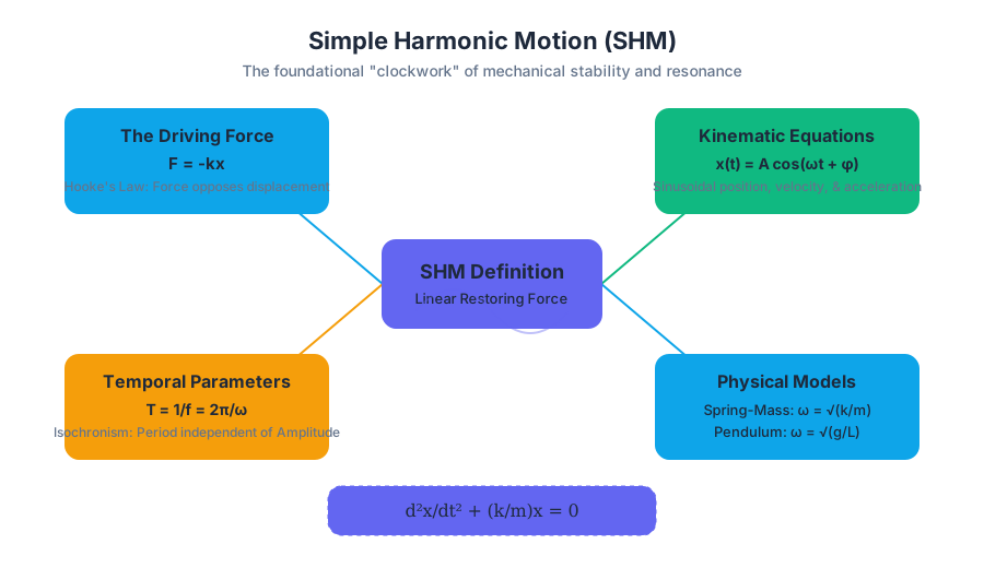
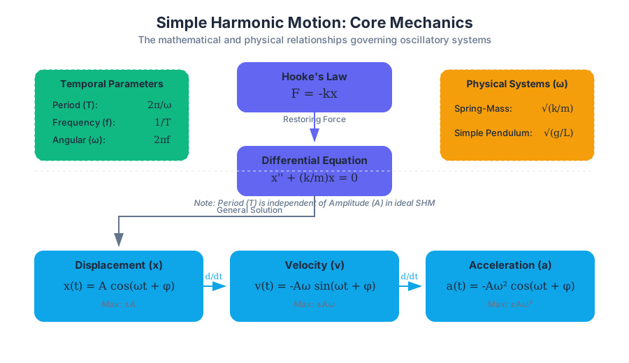
Mechanical Waves and Properties
Key concepts: Transverse and Longitudinal Waves · Wave Speed Equation · Standing Waves · Interference
The physics of wave propagation, including wave types, speed calculations, and interference patterns.
Mechanical Waves and Properties
Overview
At its most fundamental level, a mechanical wave is a disturbance that propagates through a medium—be it solid, liquid, or gas—transferring energy from one location to another without the permanent displacement of the medium's particles. Unlike electromagnetic waves, which can traverse the vacuum of space, mechanical waves are inextricably linked to the physical properties of the matter they inhabit. They rely on the elastic and inertial properties of the medium to "reset" particles to their equilibrium positions, creating the oscillatory behavior we observe as a wave.
In this deep dive, we will explore the taxonomy of waves, the rigorous mathematics governing their speed, the complex beauty of their interactions, and the specialized case of standing waves that forms the basis of musical acoustics and structural engineering.
Classification by Particle Motion: Transverse and Longitudinal
Mechanical waves are categorized primarily by the relationship between the direction of the wave's travel (propagation) and the direction of the individual particles' oscillation.
Transverse Waves
In a transverse wave, the particles of the medium oscillate perpendicularly to the direction of energy transfer. Imagine a plucked guitar string; while the wave travels down the length of the string, the string fibers move up and down.
- Crest: The point of maximum positive displacement.
- Trough: The point of maximum negative displacement.
- Polarization: A unique property of transverse waves where the oscillation can be restricted to a single plane.
Longitudinal Waves
In a longitudinal wave, the particles oscillate parallel to the direction of wave propagation. Sound waves in air are the quintessential example. Instead of peaks and valleys, these waves consist of alternating regions of high and low density.
- Compression: A region where the medium is squashed together (high pressure).
- Rarefaction: A region where the medium is stretched apart (low pressure).
| Feature | Transverse Waves | Longitudinal Waves |
|---|---|---|
| Particle Motion | Perpendicular to propagation | Parallel to propagation |
| Medium Requirement | Solids and liquid surfaces (requires shear strength) | Solids, liquids, and gases |
| Key Components | Crests and Troughs | Compressions and Rarefactions |
| Example | S-waves (Seismic), String vibrations | Sound waves, P-waves (Seismic) |
| Polarization | Possible | Impossible |
The Wave Speed Equation: A Derivation
The speed of a wave ($v$) is not arbitrary; it is a fixed property of the medium. To understand the relationship between velocity, frequency ($f$), and wavelength ($\lambda$), we must look at the kinematics of a single wave cycle.
The Wave Equation: $v = f \lambda$
Where:
- $v$ is the wave speed (m/s)
- $f$ is the frequency (Hz or $s^{-1}$)
- $\lambda$ is the wavelength (m)
Mathematical Derivation
- Velocity Definition: By definition, velocity is displacement over time: $v = \frac{\Delta x}{\Delta t}$.
- The Single Cycle: Consider the time it takes for one full wave cycle to pass a fixed point. This time is defined as the Period ($T$).
- The Distance: In the span of one period, the wave travels exactly one Wavelength ($\lambda$).
- Substitution: Substituting these into the velocity formula gives $v = \frac{\lambda}{T}$.
- Frequency Relation: Since frequency is the reciprocal of the period ($f = \frac{1}{T}$), we arrive at the final form: $v = f \lambda$.
Implementation: Simulating Wave Propagation
To visualize how these parameters interact in a computational environment, we can use Python with NumPy to model a discrete wave function over time.
import numpy as np

def simulate_wave(amplitude, frequency, wavelength, time_steps, space_steps):
    """
    Generates a 2D array representing a transverse wave moving through space.
    v = f * lambda
    """
    # Calculate wave speed and angular parameters
    velocity = frequency * wavelength
    k = 2 * np.pi / wavelength  # Wave number
    omega = 2 * np.pi * frequency # Angular frequency

    x = np.linspace(0, 10, space_steps)
    t = np.linspace(0, 2, time_steps)

    # Create a grid for space and time
    X, T = np.meshgrid(x, t)

    # Wave function: y(x, t) = A * sin(kx - wt)
    # This represents a wave traveling in the positive x direction
    wave_data = amplitude * np.sin(k * X - omega * T)

    return x, t, wave_data

# Example parameters: A=1.0, f=2Hz, lambda=0.5m
# Resulting wave speed: 1.0 m/s
x_coords, t_coords, displacement = simulate_wave(1.0, 2.0, 0.5, 100, 500)
The Principle of Superposition and Interference
When two mechanical waves meet while traveling through the same medium, they do not "bounce" off each other like billiard balls. Instead, they pass through one another, and at the point of intersection, their displacements add algebraically. This is known as the Principle of Superposition.
Constructive Interference
Occurs when waves are in phase (crests align with crests). The resulting amplitude is the sum of the individual amplitudes ($A_{total} = A_1 + A_2$).
Destructive Interference
Occurs when waves are out of phase (crests align with troughs). If the amplitudes are equal, they completely cancel each other out, resulting in zero displacement at that point.
The Math of Phase Difference
The nature of interference is determined by the phase difference ($\phi$) or the Path Difference ($\Delta L$) between two sources.
\text{Constructive Interference: } \Delta L = n\lambda \quad (n = 0, 1, 2, ...)
\text{Destructive Interference: } \Delta L = (n + \frac{1}{2})\lambda \quad (n = 0, 1, 2, ...)
| Parameter | Constructive | Destructive |
|---|---|---|
| Phase Difference | $0, 2\pi, 4\pi...$ | $\pi, 3\pi, 5\pi...$ |
| Path Difference | Integer wavelengths ($n\lambda$) | Half-integer wavelengths ($(n+0.5)\lambda$) |
| Resulting Amplitude | Maximum ($A_1 + A_2$) | Minimum ($ |
| Energy Density | Concentrated | Dissipated/Redistributed |
Standing Waves and Resonance
A standing wave is a special interference pattern formed when two waves of the same frequency and amplitude travel in opposite directions in the same medium. This usually occurs when a wave reflects off a boundary and interferes with the incoming wave.
Unlike traveling waves, standing waves do not appear to move through the medium. Instead, certain points remain stationary while others oscillate with maximum intensity.
Nodes and Antinodes
- Nodes: Points of zero displacement caused by continuous destructive interference.
- Antinodes: Points of maximum displacement caused by continuous constructive interference.
Boundary Conditions and Harmonics
The frequencies at which standing waves form are called resonant frequencies or harmonics. These are dictated by the boundary conditions of the medium.
- Fixed-Fixed (e.g., Guitar String): Both ends must be nodes.
- Fundamental ($n=1$): $L = \frac{1}{2}\lambda \rightarrow \lambda = 2L$
- Second Harmonic ($n=2$): $L = \lambda \rightarrow \lambda = L$
- General Formula: $f_n = \frac{nv}{2L}$
- Open-Closed (e.g., Organ Pipe): One end is a node, the other is an antinode.
- General Formula: $f_n = \frac{nv}{4L}$ (where $n$ is odd)
Real-World Usage: Signal Generation
In audio engineering, we often need to generate these specific harmonic frequencies. Below is a shell command using sox (Sound eXchange) to generate a fundamental frequency and its first two harmonics for a string of length $L$ where $v/2L = 440$ Hz.
# Generate 440Hz (Fundamental), 880Hz (2nd Harmonic), and 1320Hz (3rd Harmonic)
# Mix them into a single output file to simulate a complex standing wave tone
sox -n -r 44100 output.wav synth 3.0 \
    sine 440 \
    sine 880 \
    sine 1320 \
    remix -
Energy and Power in Mechanical Waves
Waves are, above all, a mechanism for energy transport. The energy of a mechanical wave is stored in both the kinetic energy of the moving particles and the potential energy of the deformed medium.
Key Insight: The power ($P$) transmitted by a wave is proportional to the square of the amplitude ($A^2$) and the square of the frequency ($f^2$).
Intensity
Intensity ($I$) is the power delivered per unit area. For a point source emitting waves in three dimensions (like a sound source), the intensity follows the Inverse Square Law:
$$I = \frac{P}{4\pi r^2}$$
This explains why sound gets significantly quieter as you move away; doubling the distance ($r$) reduces the intensity to one-fourth of its original value.
Common Pitfalls and Misconceptions
- Medium vs. Wave Velocity: A common mistake is confusing the speed of the wave ($v = f\lambda$) with the speed of the individual particles. In a transverse wave, the particles move at a speed determined by the derivative of the wave function, which changes throughout the cycle, while the wave speed remains constant.
- Frequency vs. Medium: Frequency is determined solely by the source of the wave. Once a wave is created, its frequency does not change, even if it enters a different medium. Only its speed and wavelength change.
- Sound in Vacuum: Students often forget that sound is mechanical. It requires a medium. In space, "no one can hear you scream" because there are no particles to compress or rarefy.
- Standing Wave "Movement": Standing waves do not "travel." If you track a crest, it doesn't move horizontally; it simply grows and shrinks in place.
Summary of Wave Parameters
| Parameter | Symbol | Definition | Dependency |
|---|---|---|---|
| Period | $T$ | Time for one cycle | Source |
| Frequency | $f$ | Cycles per second | Source |
| Wavelength | $\lambda$ | Distance between identical points | Source & Medium |
| Wave Speed | $v$ | Speed of energy propagation | Medium Properties |
| Amplitude | $A$ | Max displacement from equilibrium | Source Energy |
Concrete Example: Seismic Wave Analysis
During an earthquake, the Earth's crust acts as the medium for several types of mechanical waves.
- P-waves (Primary): Longitudinal waves that travel fastest and reach seismographs first.
- S-waves (Secondary): Transverse waves that travel slower and cannot pass through the liquid outer core of the Earth (since liquids have no shear strength).
Problem: A seismograph detects a P-wave traveling at $8000 \text{ m/s}$ and an S-wave traveling at $4500 \text{ m/s}$. If the S-wave arrives $20 \text{ seconds}$ after the P-wave, how far away was the earthquake?
Solution: Let $d$ be the distance. Time for P-wave: $t_p = d / 8000$ Time for S-wave: $t_s = d / 4500$ Given $t_s - t_p = 20$: $$\frac{d}{4500} - \frac{d}{8000} = 20$$ Find a common denominator or solve for $d$: $$d \left( \frac{8000 - 4500}{4500 \times 8000} \right) = 20$$ $$d \left( \frac{3500}{36,000,000} \right) = 20$$ $$d \approx 205,714 \text{ meters (or } \sim 206 \text{ km)}$$
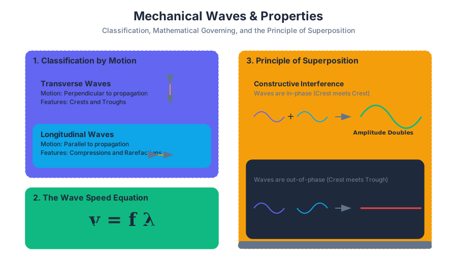
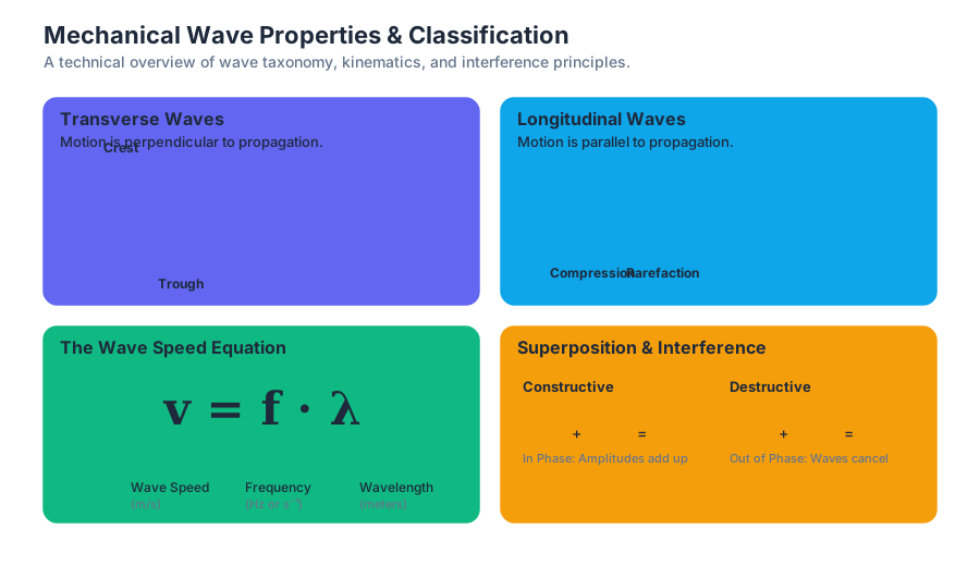
The Physics of Sound
Key concepts: Doppler Effect · Standing Waves in Tubes · Beat Frequency · Sound Intensity
A specialized look at sound waves, focusing on resonance in tubes, beats, and the Doppler effect.
The Physics of Sound
Sound is a mechanical, longitudinal wave that propagates through a medium via the periodic compression and rarefaction of molecules. Unlike electromagnetic waves, sound requires a physical substrate—be it gas, liquid, or solid—to transmit energy. In the context of fluid dynamics and classical mechanics, sound is best understood as a pressure wave. When a source vibrates, it imparts kinetic energy to adjacent particles, creating a local increase in pressure (compression) followed by a decrease (rarefaction).
The velocity of sound ($v$) is not a universal constant but depends on the elastic and inertial properties of the medium. In a fluid, it is defined by the bulk modulus ($B$) and density ($\rho$): $$v = \sqrt{\frac{B}{\rho}}$$ In the atmosphere, temperature is the primary driver of speed variance, approximated at $v \approx 331.3 \sqrt{1 + \frac{T}{273.15}}$ m/s. Understanding sound requires moving beyond simple wave propagation into the complex interactions of boundary conditions, relative motion, and interference patterns.
Standing Waves in Tubes
When sound waves are confined within a cylindrical cavity, such as a flute, a pipe organ, or a human vocal tract, they undergo reflection at the boundaries. The interference between the incident wave and the reflected wave creates standing waves. These are stationary patterns where certain points (nodes) remain at rest while others (antinodes) oscillate with maximum amplitude.
Boundary Conditions: Displacement vs. Pressure
It is critical to distinguish between displacement nodes and pressure nodes.
- At a closed end, air molecules are physically stopped by a barrier, creating a displacement node. However, because molecules pile up against this wall, this point experiences the maximum pressure fluctuation, making it a pressure antinode.
- At an open end, the air is free to move, creating a displacement antinode. Because the open end is exposed to the constant atmospheric pressure of the outside environment, it remains a pressure node.
Harmonic Series in Open and Closed Tubes
The geometry of the tube determines which wavelengths ($\lambda$) can survive through constructive interference.
| Tube Type | Boundary Conditions | Fundamental Wavelength ($\lambda_1$) | Harmonic Sequence | Allowed Harmonics ($n$) |
|---|---|---|---|---|
| Open-Open | Antinode at both ends | $2L$ | $f_n = \frac{nv}{2L}$ | $n = 1, 2, 3, \dots$ (All) |
| Open-Closed | Node at one, Antinode at other | $4L$ | $f_n = \frac{nv}{4L}$ | $n = 1, 3, 5, \dots$ (Odd only) |
| Closed-Closed | Node at both ends | $2L$ | $f_n = \frac{nv}{2L}$ | $n = 1, 2, 3, \dots$ (All) |
The End Correction Factor: In real-world acoustics, the displacement antinode at an open end does not occur exactly at the tube's exit but slightly beyond it. For a tube of radius $r$, the effective length $L_{eff}$ is approximately $L + 0.6r$ for each open end. This is why professional instrument tuning involves physical adjustments to the bore length.
Worked Example: The Pipe Organ
Consider an organ pipe that is 2.5 meters long, open at one end and closed at the other, in a room where the speed of sound is 343 m/s.
- Fundamental Frequency ($f_1$): $$f_1 = \frac{v}{4L} = \frac{343}{4(2.5)} = 34.3 \text{ Hz}$$
- Third Harmonic ($f_3$): $$f_3 = 3 \times f_1 = 102.9 \text{ Hz}$$ Note that the second harmonic ($n=2$) cannot exist in this configuration because the boundary conditions (Node-Antinode) cannot be satisfied by a full half-wavelength.
/*
 * low-level implementation: Harmonic Frequency Calculator
 * This C program calculates the first N harmonics for a given tube length
 * and temperature, accounting for the type of tube boundary.
 */

#include <stdio.h>
#include <math.h>

#define ADIABATIC_INDEX 1.4
#define GAS_CONSTANT 287.05 // J/(kg*K) for air

double calculate_speed_of_sound(double temp_celsius) {
    double temp_kelvin = temp_celsius + 273.15;
    return sqrt(ADIABATIC_INDEX * GAS_CONSTANT * temp_kelvin);
}

void print_harmonics(double L, double v, int open_both_ends, int count) {
    printf("Speed of Sound: %.2f m/s\n", v);
    printf("Fundamental and Overtones:\n");

    for (int n = 1; n <= count; n++) {
        if (open_both_ends) {
            double f = (n * v) / (2 * L);
            printf("Harmonic %d: %.2f Hz\n", n, f);
        } else {
            // Only odd harmonics for open-closed tubes
            int harmonic_num = 2 * n - 1;
            double f = (harmonic_num * v) / (4 * L);
            printf("Harmonic %d: %.2f Hz\n", harmonic_num, f);
        }
    }
}

int main() {
    double length = 1.2; // meters
    double temp = 20.0;  // Celsius
    double v = calculate_speed_of_sound(temp);

    printf("--- Open-Open Tube ---\n");
    print_harmonics(length, v, 1, 5);

    printf("\n--- Open-Closed Tube ---\n");
    print_harmonics(length, v, 0, 5);

    return 0;
}
The Doppler Effect
The Doppler Effect is the observed change in frequency of a wave when there is relative motion between the source and the observer. It is not a change in the frequency emitted by the source, but rather a result of the "bunching up" or "stretching out" of wave fronts in the medium.
The General Doppler Equation
The perceived frequency $f'$ is related to the source frequency $f_s$ by: $$f' = f_s \left( \frac{v \pm v_o}{v \mp v_s} \right)$$ Where:
- $v$: Speed of sound in the medium.
- $v_o$: Velocity of the observer.
- $v_s$: Velocity of the source.
Sign Convention Logic:
- The numerator $(v \pm v_o)$ concerns the observer. Use + if the observer moves toward the source (increasing perceived frequency).
- The denominator $(v \mp v_s)$ concerns the source. Use - if the source moves toward the observer (decreasing the denominator, thus increasing $f'$).
| Scenario | Numerator Sign | Denominator Sign | Resulting $f'$ |
|---|---|---|---|
| Observer moving toward stationary Source | $+$ | $v$ | $f' > f_s$ |
| Source moving toward stationary Observer | $v$ | $-$ | $f' > f_s$ |
| Both moving away from each other | $-$ | $+$ | $f' < f_s$ |
| Source moving at $v_s = v$ | $v$ | $0$ | $f' \to \infty$ (Shockwave) |
Derivation for a Moving Source
Consider a source moving toward a stationary observer at velocity $v_s$. In one period $T$, the source moves a distance $d_s = v_s T$. The wave itself travels $d_w = v T$. The new wavelength $\lambda'$ is the distance between successive wave fronts: $$\lambda' = d_w - d_s = (v - v_s)T$$ Since $T = 1/f_s$ and $f' = v/\lambda'$: $$f' = \frac{v}{(v - v_s)/f_s} = f_s \left( \frac{v}{v - v_s} \right)$$ This confirms that as the source approaches, the wavelength decreases, causing the pitch to rise.
Applications and Extensions
- Astronomy (Redshift/Blueshift): While light follows relativistic Doppler equations, the principle is the same: objects moving away appear "redder" (lower frequency).
- Medical Imaging: Doppler Ultrasound measures the velocity of blood flow by detecting the frequency shift of sound waves reflected off moving red blood cells.
- Sonic Booms: When $v_s > v$, the wave fronts overlap to form a conical pressure ridge known as a Mach cone. The angle of this cone is $\sin \theta = v / v_s = 1/M$, where $M$ is the Mach number.
Beat Frequency
When two sound waves of slightly different frequencies, $f_1$ and $f_2$, overlap at the same point in space, they interfere. Because their frequencies differ, they alternate between being in-phase (constructive interference) and out-of-phase (destructive interference). This results in a periodic variation in volume called beats.
Mathematical Derivation
Assume two waves of equal amplitude $A$: $$y_1 = A \sin(2\pi f_1 t)$$ $$y_2 = A \sin(2\pi f_2 t)$$ Using the trigonometric identity $\sin \alpha + \sin \beta = 2 \sin(\frac{\alpha+\beta}{2}) \cos(\frac{\alpha-\beta}{2})$: $$y_{total} = \left[ 2A \cos\left(2\pi \frac{f_1 - f_2}{2} t\right) \right] \sin\left(2\pi \frac{f_1 + f_2}{2} t\right)$$ The term in the brackets represents a slowly varying amplitude (the envelope). The frequency of this envelope is $\frac{f_1 - f_2}{2}$. However, because a "beat" is heard at every maximum amplitude (both positive and negative peaks of the cosine), the human ear perceives two beats per cycle of the envelope. Therefore, the Beat Frequency ($f_b$) is: $$f_b = |f_1 - f_2|$$
Usage in Instrument Tuning
Musicians use beats to tune instruments to a reference pitch (like a tuning fork). If a piano string and a 440 Hz tuning fork produce 3 beats per second, the string is vibrating at either 437 Hz or 443 Hz. The tuner then tightens or loosens the string; if the beat frequency decreases, they are moving toward the correct pitch.
# Mathematical representation and signal generation for Beats
import numpy as np
import matplotlib.pyplot as plt

def generate_beats(f1, f2, duration, fs=44100):
    t = np.linspace(0, duration, int(fs * duration))
    # Two sine waves with slightly different frequencies
    wave1 = np.sin(2 * np.pi * f1 * t)
    wave2 = np.sin(2 * np.pi * f2 * t)

    # Superposition
    combined = wave1 + wave2

    # The theoretical beat frequency
    f_beat = abs(f1 - f2)
    print(f"Theoretical Beat Frequency: {f_beat} Hz")
    return t, combined

# Parameters: 440Hz (A4) and 444Hz
t, signal = generate_beats(440, 444, 0.5)

# Plotting the first 0.25 seconds to see the envelope
plt.figure(figsize=(10, 4))
plt.plot(t, signal)
plt.title("Interference Pattern (Beats)")
plt.xlabel("Time (s)")
plt.ylabel("Amplitude")
plt.grid(True)
plt.show()
Sound Intensity and the Decibel Scale
Sound intensity ($I$) is the rate at which energy is transported per unit area perpendicular to the direction of propagation. $$I = \frac{P}{A} = \frac{P}{4\pi r^2}$$ This Inverse Square Law implies that if you double your distance from a point source, the intensity drops to one-fourth of its original value.
The Logarithmic Nature of Hearing
The human ear can detect intensities ranging from $10^{-12} \text{ W/m}^2$ (the Threshold of Hearing) to over $10 \text{ W/m}^2$ (the threshold of pain). Because this range spans 13 orders of magnitude, we use a logarithmic scale called the Sound Intensity Level ($\beta$), measured in Decibels (dB).
$$\beta = 10 \log_{10} \left( \frac{I}{I_0} \right)$$ Where $I_0 = 10^{-12} \text{ W/m}^2$.
| Sound Source | Intensity ($W/m^2$) | Intensity Level (dB) | Perception |
|---|---|---|---|
| Threshold of Hearing | $10^{-12}$ | 0 | Barely audible |
| Rustling Leaves | $10^{-11}$ | 10 | Very quiet |
| Normal Conversation | $10^{-6}$ | 60 | Comfortable |
| Power Lawn Mower | $10^{-2}$ | 100 | Potentially damaging |
| Jet Engine (30m) | $10^{2}$ | 140 | Painful / Immediate damage |
Key Insight: Every increase of 10 dB represents a 10-fold increase in intensity. However, a 10 dB increase is generally perceived by the human ear as only a "doubling" of loudness. This is a physiological artifact described by the Weber-Fechner Law.
Combining Sound Sources
If you have two independent sound sources (e.g., two violins) playing at 60 dB each, the total intensity level is not 120 dB. Instead, you must sum the intensities:
- $I_{total} = I_1 + I_2$
- Since $I_1 = I_2 = 10^{-6} \text{ W/m}^2$, $I_{total} = 2 \times 10^{-6} \text{ W/m}^2$.
- $\beta_{total} = 10 \log_{10} (2 \times 10^{-6} / 10^{-12}) = 10 \log_{10} (2 \times 10^6) \approx 63 \text{ dB}$. Doubling the power of a sound source results in a mere 3 dB increase.
# Real-world usage: Using FFmpeg to analyze or generate sound properties
# Generate a 440Hz tone and a 441Hz tone to hear a 1Hz beat
ffmpeg -f lavfi -i "sine=frequency=440:duration=5" -f lavfi -i "sine=frequency=441:duration=5" \
-filter_complex "amix=inputs=2" output_beats.wav

# Measure the decibel level (RMS) of an existing audio file
ffmpeg -i output_beats.wav -filter:a volumedetect -f null /dev/null
Common Pitfalls and Misconceptions
- Medium Dependency: A common mistake is assuming the speed of sound is constant. In underwater acoustics (SONAR), the speed of sound varies significantly with salinity and depth, creating "shadow zones" where sound waves refract away, making objects invisible to sonar.
- Frequency vs. Speed: Increasing the frequency of a sound wave does not increase its speed. Speed is a property of the medium. $v = f\lambda$; if $f$ increases, $\lambda$ must decrease proportionally.
- The "Vacuum" Myth: Science fiction often depicts loud explosions in space. Since sound is a mechanical wave requiring a medium for particle-to-particle interaction, space is silent.
- Doppler Sign Errors: Students often confuse the signs in the Doppler formula. Remember: Toward = Higher Frequency. If your calculation results in a lower frequency for an approaching source, your signs are reversed.
- Longitudinal Wave: A wave where particle displacement is parallel to the direction of energy transport.
- Node: A point in a standing wave with zero displacement (or zero pressure change).
- Antinode: A point in a standing wave with maximum displacement (or maximum pressure change).
- Fundamental Frequency: The lowest frequency of a standing wave that can be supported by a given geometry.
- Harmonics: Integer multiples of the fundamental frequency.
- Beat Frequency: The absolute difference between two interfering frequencies ($|f_1 - f_2|$).
- Intensity: Power per unit area ($W/m^2$).
- Decibel (dB): A logarithmic unit used to express the ratio of a sound's intensity to a reference level.
- Doppler Shift: The change in frequency caused by relative motion between source and observer.
- Bulk Modulus: A measure of a substance's resistance to uniform compression, key to determining sound speed in fluids.
- Why do open-closed tubes only produce odd harmonics?
- If a source moves away from an observer at the speed of sound, what is the perceived frequency?
- Calculate the decibel level of a sound with an intensity of $10^{-4} \text{ W/m}^2$.
- Two tuning forks of 256 Hz and 260 Hz are struck simultaneously. How many beats are heard in 5 seconds?
- How does the speed of sound change if the air temperature rises from 0°C to 30°C?
- Explain the difference between a pressure node and a displacement node at the open end of a pipe.
Key Formulas to Memorize:
- Speed in gas: $v \approx 331 + 0.6T$
- Open Tube: $f_n = \frac{nv}{2L}$
- Closed Tube: $f_n = \frac{(2n-1)v}{4L}$
- Doppler: $f' = f \frac{v \pm v_o}{v \mp v_s}$
- Intensity Level: $\beta = 10 \log \frac{I}{I_0}$
- Beats: $f_b = |f_1 - f_2|$
Problem Solving Strategy:
- Identify the Medium: Check for temperature or material properties to find $v$.
- Check Boundaries: Is the tube open at both ends or closed at one? This dictates the harmonic formula.
- Determine Motion: For Doppler problems, draw a vector diagram. Define the "positive" direction from observer to source to keep signs consistent.
- Logarithmic Math: Remember that adding 3 dB doubles the intensity, and adding 10 dB increases intensity by 10x.
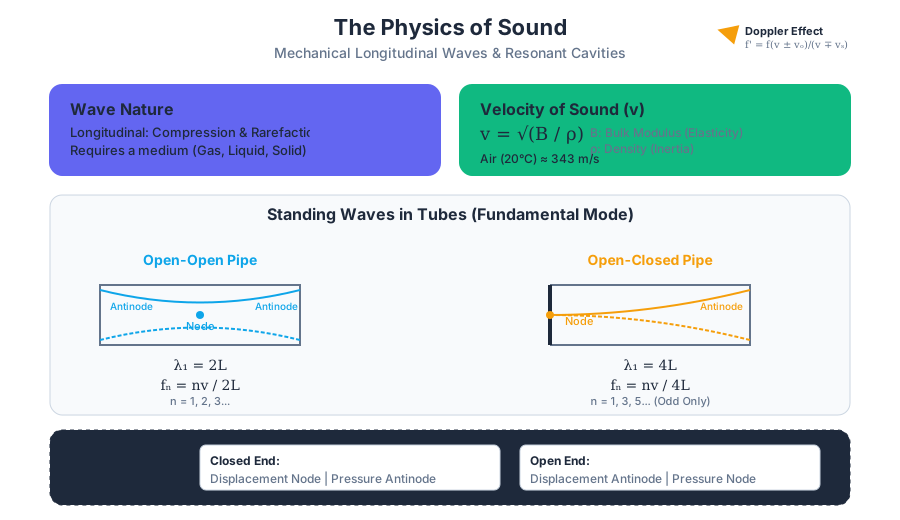
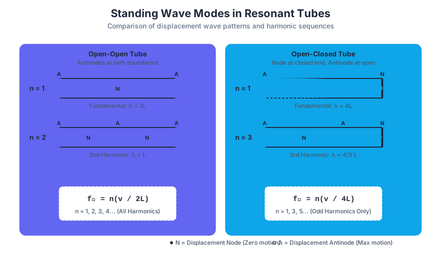
Static Electricity and Electric Force
Key concepts: Electric Charge · Conservation of Charge · Coulomb's Law · Conductors and Insulators
Introduction to electric charge, methods of charging, and Coulomb's Law.
Static Electricity and Electric Force
Electrostatics is the branch of physics that deals with the phenomena and properties of stationary or slow-moving electric charges. While the term "static" implies a lack of motion, the field is fundamentally about the potential for interaction—the invisible "action-at-a-distance" that governs everything from the structure of the atom to the catastrophic discharge of a lightning bolt.
The Nature of Electric Charge
At its most fundamental level, Electric Charge is an intrinsic physical property of matter that causes it to experience a force when placed in an electromagnetic field. Unlike mass, which is always positive and only attractive in a Newtonian sense, electric charge comes in two distinct varieties: positive and negative.
The Quantization of Charge
In the macroscopic world, charge appears continuous. However, at the subatomic scale, charge is quantized. This means it exists only in discrete integer multiples of a fundamental unit, known as the elementary charge ($e$).
The Quantization Principle: The charge $q$ of any object is given by $q = ne$, where $n$ is an integer (positive or negative) and $e \approx 1.602 \times 10^{-19}$ Coulombs.
Fundamental Particles and Charge
The primary carriers of charge in ordinary matter are protons and electrons. While their masses differ by nearly three orders of magnitude, their charge magnitudes are identical.
| Particle | Charge (C) | Mass (kg) | Location |
|---|---|---|---|
| Proton | $+1.602 \times 10^{-19}$ | $1.673 \times 10^{-27}$ | Nucleus |
| Electron | $-1.602 \times 10^{-19}$ | $9.109 \times 10^{-31}$ | Orbitals/Shells |
| Neutron | $0$ | $1.675 \times 10^{-27}$ | Nucleus |
# Low-level implementation: Simulating Charge Quantization and Basic Interaction
import math

class Particle:
    ELEMENTARY_CHARGE = 1.602176634e-19  # Coulombs

    def __init__(self, name, n_electrons, n_protons):
        self.name = name
        # Charge is quantized: net charge = (protons - electrons) * e
        self.net_charge = (n_protons - n_electrons) * self.ELEMENTARY_CHARGE

    def get_charge_in_coulombs(self):
        return self.net_charge

    def calculate_electrostatic_force(self, other_particle, distance):
        """
        Calculates the magnitude of force between two particles using Coulomb's Law.
        F = k * |q1 * q2| / r^2
        """
        k = 8.9875517923e9  # Coulomb's constant in N·m²/C²
        if distance <= 0:
            raise ValueError("Distance must be greater than zero.")

        force = k * abs(self.net_charge * other_particle.net_charge) / (distance**2)
        return force

# Example usage: Force between a proton and an electron at Bohr radius
proton = Particle("Proton", 0, 1)
electron = Particle("Electron", 1, 0)
bohr_radius = 5.29177e-11 # meters

force = proton.calculate_electrostatic_force(electron, bohr_radius)
print(f"Force at Bohr radius: {force:.2e} Newtons")
Conservation of Charge
The Law of Conservation of Charge is a foundational pillar of physics. It states that the net electric charge of an isolated system remains constant regardless of any internal changes. Charge is neither created nor destroyed; it is merely transferred from one body to another.
Mechanics of Transfer
In most terrestrial applications, "charging" an object involves the movement of electrons. Protons are bound tightly within the atomic nucleus by the strong nuclear force; moving them would require nuclear levels of energy. Electrons, particularly those in the outer "valence" shells of conductors, are much more mobile.
- Negative Charge Acquisition: An object gains electrons.
- Positive Charge Acquisition: An object loses electrons (leaving behind uncompensated protons).
Conductors, Insulators, and Semiconductors
The behavior of static charge on an object depends entirely on the material's internal atomic structure and how easily electrons can migrate through the lattice.
| Material Type | Electron Mobility | Mechanism | Common Examples |
|---|---|---|---|
| Conductor | High | "Sea of electrons" move freely across the lattice. | Copper, Silver, Aluminum, Salt Water |
| Insulator | Low | Electrons are tightly bound to specific atoms/molecules. | Rubber, Glass, Plastic, Dry Wood |
| Semiconductor | Variable | Conductivity depends on impurities (doping) or temperature. | Silicon, Germanium, Gallium Arsenide |
| Superconductor | Infinite | Zero resistance below a critical temperature ($T_c$). | Mercury (<4.2K), YBCO |
Charge Distribution in Conductors
In a conductor, like charges repel each other. Consequently, any excess charge placed on a conductor will migrate to the outer surface to maximize the distance between individual charges. Inside the bulk of a static conductor, the net electric field is always zero.
Mechanisms of Charging
Understanding how objects become "static" requires looking at the interface of materials.
1. The Triboelectric Effect (Charging by Friction)
When two different materials are brought into contact and then separated, one may "steal" electrons from the other. This is governed by the Triboelectric Series, a ranking of materials based on their electron affinity.
| Material | Tendency |
|---|---|
| Rabbit Fur | Highly Positive (Loses Electrons) |
| Glass | Positive |
| Human Hair | Positive |
| Silk | Neutral / Slightly Negative |
| Hard Rubber | Negative |
| PVC / Teflon | Highly Negative (Gains Electrons) |
2. Charging by Conduction (Contact)
This involves the direct physical transfer of electrons from a charged object to a neutral (or differently charged) object. If a negatively charged rod touches a neutral metal sphere, electrons flow onto the sphere until a state of equilibrium is reached.
3. Charging by Induction
Induction is a method used to charge an object without touching it.
- Bring a charged object (e.g., a negative rod) near a neutral conductor.
- The electrons in the conductor are repelled to the far side (Polarization).
- "Ground" the far side of the conductor, allowing the repelled electrons to escape to the Earth.
- Remove the ground, then remove the rod. The conductor is now left with a net positive charge.
Coulomb’s Law
Coulomb's Law provides the mathematical framework for calculating the magnitude and direction of the force between two stationary point charges.
Coulomb's Law: The magnitude of the electric force $F$ between two point charges $q_1$ and $q_2$ is directly proportional to the product of the charges and inversely proportional to the square of the distance $r$ between them.
\mathbf{F}_{12} = k \frac{q_1 q_2}{r^2} \mathbf{\hat{r}}_{21}
Where:
- $F$ is the force in Newtons (N).
- $q_1, q_2$ are the charges in Coulombs (C).
- $r$ is the separation distance in meters (m).
- $k$ is Coulomb's constant, $k = \frac{1}{4\pi\epsilon_0} \approx 8.99 \times 10^9 \text{ N}\cdot\text{m}^2/\text{C}^2$.
- $\epsilon_0$ is the permittivity of free space ($\approx 8.854 \times 10^{-12} \text{ C}^2/\text{N}\cdot\text{m}^2$).
Vector Nature and Superposition
Electrostatic force is a vector. If multiple charges are present, the net force on any single charge is the vector sum of the individual forces exerted by all other charges. This is known as the Principle of Superposition.
Comparison: Electrostatic vs. Gravitational Force
Coulomb's Law bears a striking resemblance to Newton's Law of Universal Gravitation. Both are inverse-square laws, but they differ significantly in scale and nature.
| Feature | Electrostatic Force ($F_e$) | Gravitational Force ($F_g$) |
|---|---|---|
| Equation | $k \frac{q_1 q_2}{r^2}$ | $G \frac{m_1 m_2}{r^2}$ |
| Constant | $8.99 \times 10^9$ | $6.67 \times 10^{-11}$ |
| Nature | Attractive or Repulsive | Always Attractive |
| Strength | Extremely Strong | Extremely Weak |
| Range | Infinite | Infinite |
Proof of Strength: Compare the $F_e$ and $F_g$ between two protons. The ratio $F_e / F_g \approx 10^{36}$. Gravity is only dominant on a cosmic scale because large bodies are usually electrically neutral.
Worked Example: The Three-Charge System
Consider three point charges arranged in a line:
- $q_1 = +2.0 \mu\text{C}$ at $x = 0$
- $q_2 = -3.0 \mu\text{C}$ at $x = 0.4\text{ m}$
- $q_3 = -5.0 \mu\text{C}$ at $x = 1.2\text{ m}$
Goal: Find the net force on $q_2$.
-
Force from $q_1$ on $q_2$ ($F_{12}$): Since $q_1$ is positive and $q_2$ is negative, the force is attractive. $q_2$ is pulled toward $x=0$ (the negative x-direction). $F_{12} = k \frac{|q_1 q_2|}{r_{12}^2} = (8.99 \times 10^9) \frac{(2 \times 10^{-6})(3 \times 10^{-6})}{(0.4)^2} = 0.337 \text{ N}$ (Left)
-
Force from $q_3$ on $q_2$ ($F_{32}$): Since both $q_3$ and $q_2$ are negative, the force is repulsive. $q_2$ is pushed away from $q_3$ (toward the negative x-direction). $r_{32} = 1.2 - 0.4 = 0.8\text{ m}$ $F_{32} = k \frac{|q_3 q_2|}{r_{32}^2} = (8.99 \times 10^9) \frac{(5 \times 10^{-6})(3 \times 10^{-6})}{(0.8)^2} = 0.211 \text{ N}$ (Left)
-
Net Force ($F_{net}$): Both forces point in the same direction. $F_{net} = 0.337 + 0.211 = 0.548 \text{ N}$ in the $-x$ direction.
# Real-world usage: Using a CLI tool (units) to verify constants and conversions
# This demonstrates how an engineer might check the permittivity of free space

# Check the value of the Coulomb constant k in SI units
units "1 / (4 * pi * epsilon0)" "N m^2 / C^2"

# Output would be:
#   * 8987551787.37
#   / 1.11265005605e-10

# Calculate the force between 1C and 1C at 1m
units "coulomb_constant * 1 coulomb^2 / (1 meter)^2" "newtons"
# Output: 8.9875518e+09 newtons
Common Pitfalls and Misconceptions
- The "Static" Misnomer: Static electricity doesn't mean the charges don't move; it means they are not part of a continuous, closed-loop current. A spark is a very rapid movement of "static" charge.
- Mass vs. Charge: Students often confuse the behavior of electrons and protons. Remember: In solids, only electrons move. If an object is positively charged, it has lost electrons, not gained protons.
- The Inverse Square Law: Doubling the distance doesn't halve the force; it reduces it to one-fourth ($1/2^2$). Tripling the distance reduces it to one-ninth.
- Permittivity of the Medium: Coulomb's constant $k$ is for a vacuum. If charges are in water or oil, the force is significantly reduced because the medium polarizes and partially cancels the field. This is why the formula often uses $\epsilon$ instead of $\epsilon_0$.
Advanced Concept: Polarization in Insulators
While insulators do not allow electrons to flow across the material, they can still experience electrostatic effects through Polarization. When a charged object is brought near an insulator, the individual molecules within the insulator distort. The electron clouds shift slightly away from (or toward) the external charge.
This creates a layer of surface charge that allows a neutral insulator (like a balloon) to stick to a neutral wall. The balloon's charge polarizes the wall's molecules, creating an attractive force between the balloon and the shifted charges in the wall.
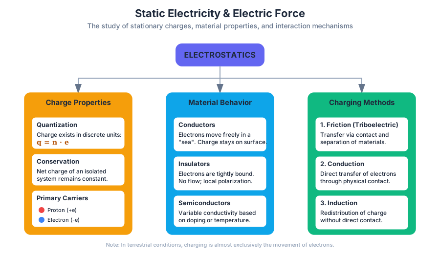
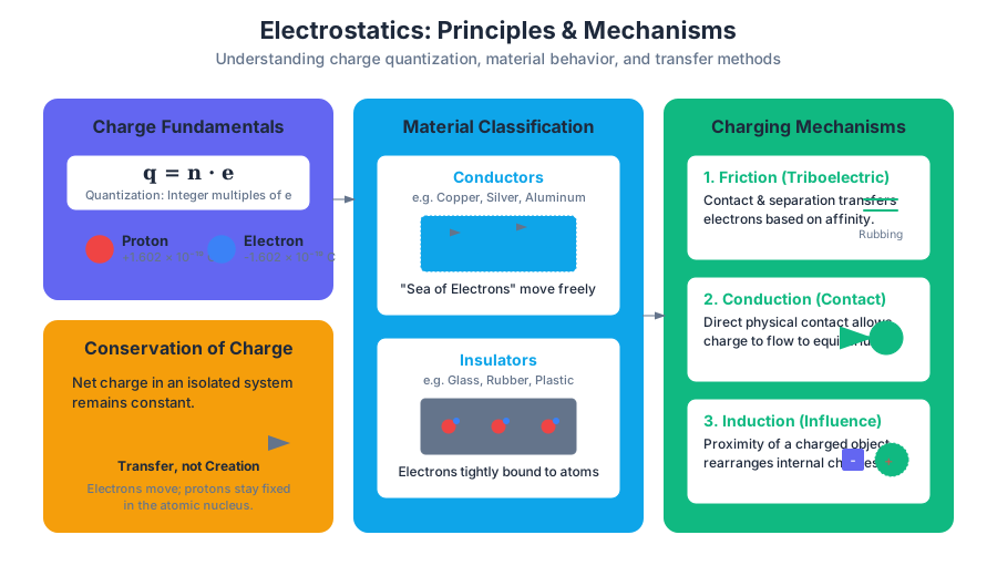
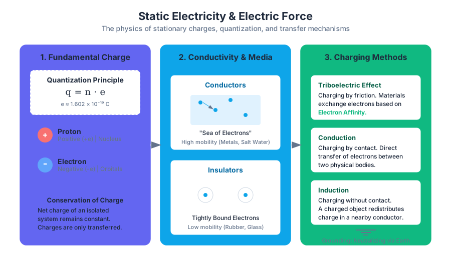
Direct Current (DC) Circuits
Key concepts: Ohm's Law (V=IR) · Series and Parallel Resistors · Electric Power · Ammeters and Voltmeters
Analyzing the flow of electric current through circuits using Ohm's Law and circuit rules.
Direct Current (DC) Circuits
Direct Current (DC) circuits represent the foundational architecture of modern electronics. Unlike Alternating Current (AC), where the flow of charge periodically reverses direction, DC maintains a constant unidirectional flow. This stability makes it the preferred medium for digital logic, battery-powered systems, and the internal rails of almost every computing device in existence. To master DC circuits is to understand the fundamental interplay between energy, charge, and resistance.
The Foundations: Charge, Current, and Potential
Before diving into specific laws, we must establish the physical quantities that define a circuit. A circuit is essentially a closed loop through which charge ($Q$) flows. This flow is driven by a potential difference ($V$), often provided by a battery or power supply, which acts as a "pump" for electrons.
| Parameter | Symbol | Unit | Physical Interpretation |
|---|---|---|---|
| Voltage | $V$ | Volts (V) | The electrical potential energy per unit charge. |
| Current | $I$ | Amperes (A) | The rate of flow of electric charge ($I = dQ/dt$). |
| Resistance | $R$ | Ohms ($\Omega$) | The opposition to the flow of electric current. |
| Conductance | $G$ | Siemens (S) | The ease with which current flows ($G = 1/R$). |
The Principle of Conventional Current: By historical convention (established by Benjamin Franklin), current is defined as the flow of positive charge. In reality, in metallic conductors, it is the negatively charged electrons that move. Thus, conventional current flows from the positive terminal to the negative terminal, while actual electron flow is the reverse.
Ohm’s Law: The Governing Equation
Ohm’s Law is the constitutive relation for a linear resistor. It states that the current through a conductor between two points is directly proportional to the voltage across the two points.
The Mathematical Formulation
The macroscopic form of Ohm's Law is: $$V = I \cdot R$$
However, for a deeper understanding, we look at the microscopic form, which relates the current density ($\mathbf{J}$) to the electric field ($\mathbf{E}$): $$\mathbf{J} = \sigma \mathbf{E}$$ where $\sigma$ is the conductivity of the material. This derivation highlights that resistance is not just a value on a component, but a property derived from the material's geometry and intrinsic resistivity ($\rho = 1/\sigma$).
Derivation of Resistance from Geometry
For a uniform conductor of length $L$ and cross-sectional area $A$: $$R = \rho \frac{L}{A}$$ This explains why longer wires have higher resistance and thicker wires have lower resistance—a crucial consideration in high-power DC distribution.
Kirchhoff’s Laws: The Conservation Principles
While Ohm's Law describes individual components, Kirchhoff’s Laws describe how those components interact within a network. They are the electrical equivalents of the conservation of charge and the conservation of energy.
Kirchhoff’s Current Law (KCL)
Theorem: The algebraic sum of currents entering a node (or a closed boundary) is zero. $$\sum_{k=1}^{n} I_k = 0$$ KCL is a statement of the Conservation of Charge. Since charge cannot build up at a point in a steady-state DC circuit, every electron entering a junction must leave it.
Kirchhoff’s Voltage Law (KVL)
Theorem: The algebraic sum of all voltages around any closed loop in a circuit is zero. $$\sum_{k=1}^{n} V_k = 0$$ KVL is a statement of the Conservation of Energy. If a charge travels in a complete loop and returns to its starting point, it must have the same potential energy it started with.
Circuit Configurations: Series and Parallel
Analyzing complex circuits requires simplifying networks into "equivalent" resistances.
Series Configurations
In a series circuit, components are connected end-to-end, forming a single path for current.
- Current is constant: $I_{total} = I_1 = I_2 = ... = I_n$.
- Voltages add up: $V_{total} = V_1 + V_2 + ... + V_n$.
- Equivalent Resistance: $R_{eq} = \sum R_i$.
Parallel Configurations
In a parallel circuit, components are connected across the same two nodes.
- Voltage is constant: $V_{total} = V_1 = V_2 = ... = V_n$.
- Currents add up: $I_{total} = I_1 + I_2 + ... + I_n$.
- Equivalent Resistance: $\frac{1}{R_{eq}} = \sum \frac{1}{R_i}$.
| Feature | Series Circuit | Parallel Circuit |
|---|---|---|
| Current Path | Single path | Multiple paths |
| Current Value | Same through all resistors | Divided among branches |
| Voltage Value | Divided across resistors | Same across all branches |
| Failure Result | One break stops all current | One break only affects that branch |
| Total Resistance | $R_{eq} >$ largest individual $R$ | $R_{eq} <$ smallest individual $R$ |
Implementation: Simulating a Resistor Network
To analyze these circuits computationally, we often use the Nodal Analysis method, which applies KCL at each node. Below is a low-level implementation in C that solves for the equivalent resistance of a simple series-parallel ladder.
#include <stdio.h>

/**
 * @brief Calculates the equivalent resistance of a DC network.
 * This example assumes a simple ladder: (R1 in series with (R2 parallel R3))
 */

typedef struct {
    double r1; // Series resistor
    double r2; // Parallel branch 1
    double r3; // Parallel branch 2
} LadderNetwork;

double calculate_equivalent_resistance(LadderNetwork net) {
    // Step 1: Calculate parallel portion (R2 || R3)
    // Formula: (R2 * R3) / (R2 + R3)
    double r_parallel = (net.r2 * net.r3) / (net.r2 + net.r3);

    // Step 2: Add the series resistor R1
    double r_total = net.r1 + r_parallel;

    return r_total;
}

int main() {
    LadderNetwork myCircuit = {100.0, 200.0, 200.0}; // Ohms
    double result = calculate_equivalent_resistance(myCircuit);

    printf("Network Configuration:\n");
    printf("R1: %.2f Ohms (Series)\n", myCircuit.r1);
    printf("R2: %.2f Ohms (Parallel Branch A)\n", myCircuit.r2);
    printf("R3: %.2f Ohms (Parallel Branch B)\n", myCircuit.r3);
    printf("------------------------------------\n");
    printf("Equivalent Resistance: %.2f Ohms\n", result);

    return 0;
}
Electric Power and Joule Heating
Electric power ($P$) is the rate at which electrical energy is transferred by an electric circuit. In a resistor, this energy is converted into heat—a phenomenon known as Joule Heating.
The Power Formulas
Using Ohm's Law, we can derive three equivalent expressions for power:
- Primary: $P = V \cdot I$
- Current-centric: $P = I^2 \cdot R$ (Useful for series circuits)
- Voltage-centric: $P = \frac{V^2}{R}$ (Useful for parallel circuits)
Derivation of the $I^2R$ Relation
Work (W) = V \cdot Q
Power (P) = \frac{dW}{dt} = V \cdot \frac{dQ}{dt} = V \cdot I
Substitute V = IR:
P = (IR) \cdot I = I^2R
This relationship is critical in power distribution. To minimize power loss ($I^2R$) in transmission lines, engineers increase the voltage ($V$) to decrease the current ($I$) for a given power level.
Measurement: Ammeters and Voltmeters
To observe these theoretical values in the real world, we use measurement instruments. However, the act of measuring a circuit inevitably changes it.
Ammeters
An Ammeter measures current.
- Connection: Must be connected in series with the component.
- Ideal Characteristic: Zero internal resistance ($R_a = 0$).
- Real-world Pitfall: If an ammeter has significant resistance, it reduces the current it is trying to measure (Loading Effect).
Voltmeters
A Voltmeter measures potential difference.
- Connection: Must be connected in parallel with the component.
- Ideal Characteristic: Infinite internal resistance ($R_v = \infty$).
- Real-world Pitfall: If a voltmeter has low resistance, it draws current away from the circuit branch, lowering the measured voltage.
| Instrument | Ideal Resistance | Connection Type | Measured Quantity |
|---|---|---|---|
| Ammeter | $0$ | Series | Current (Flow) |
| Voltmeter | $\infty$ | Parallel | Potential (Pressure) |
| Ohmmeter | N/A | Parallel (Powered Off) | Resistance |
Advanced Analysis: The Loading Effect
When using a real voltmeter, we create a parallel path. If the circuit's Thevenin resistance is high, the voltmeter's resistance ($R_m$) significantly alters the total resistance.
import numpy as np
import matplotlib.pyplot as plt

def measured_voltage(v_source, r_source, r_meter):
    """
    Calculates the voltage measured by a real voltmeter.
    v_source: The actual voltage to be measured
    r_source: The internal resistance of the circuit being measured
    r_meter: The internal resistance of the voltmeter
    """
    # The meter and source resistance form a voltage divider
    return v_source * (r_meter / (r_source + r_meter))

# Simulation: Measuring a 10V source with 10k Ohm internal resistance
r_src = 10000
v_src = 10.0
meter_resistances = np.logspace(3, 7, 100) # 1k to 10M Ohms
measured_vals = [measured_voltage(v_src, r_src, rm) for rm in meter_resistances]

plt.figure(figsize=(10, 5))
plt.semilogx(meter_resistances, measured_vals, label="Measured Voltage")
plt.axhline(y=10, color='r', linestyle='--', label="Ideal Voltage (10V)")
plt.xlabel("Voltmeter Internal Resistance (Ohms)")
plt.ylabel("Voltage Reading (V)")
plt.title("The Loading Effect: Voltmeter Resistance vs. Accuracy")
plt.legend()
plt.grid(True, which="both", ls="-")
plt.show()
Common Pitfalls in DC Analysis
- Short Circuits: Connecting a wire directly across a voltage source ($R \approx 0$). According to $I = V/R$, the current approaches infinity, leading to heat, fire, or component failure.
- Open Circuits: A break in the path ($R = \infty$). No current flows, but the full source voltage may still be present across the break.
- Grounding Misconceptions: "Ground" is simply a reference point (0V). It is not a magical sink for electrons, but a node we choose to call zero for the sake of calculation.
- Power Rating Overlook: Resistors are rated in Watts. Even if the resistance is correct, exceeding the power rating ($I^2R$) will cause the component to burn out.
Worked Example: Multi-Loop Analysis
Problem: A 12V battery is connected to a 4$\Omega$ resistor in series with a parallel combination of a 6$\Omega$ and a 12$\Omega$ resistor. Find the total current and the power dissipated by the 6$\Omega$ resistor.
Step 1: Find Equivalent Resistance ($R_{eq}$)
- Parallel part: $R_p = \frac{6 \cdot 12}{6 + 12} = \frac{72}{18} = 4\Omega$.
- Total resistance: $R_{total} = R_{series} + R_p = 4\Omega + 4\Omega = 8\Omega$.
Step 2: Find Total Current ($I_{total}$)
- $I_{total} = \frac{V}{R_{total}} = \frac{12V}{8\Omega} = 1.5A$.
Step 3: Find Voltage across the Parallel Branch ($V_p$)
- $V_p = I_{total} \cdot R_p = 1.5A \cdot 4\Omega = 6V$.
Step 4: Find Power in the 6$\Omega$ Resistor
- $P = \frac{V_p^2}{R} = \frac{6^2}{6} = \frac{36}{6} = 6W$.
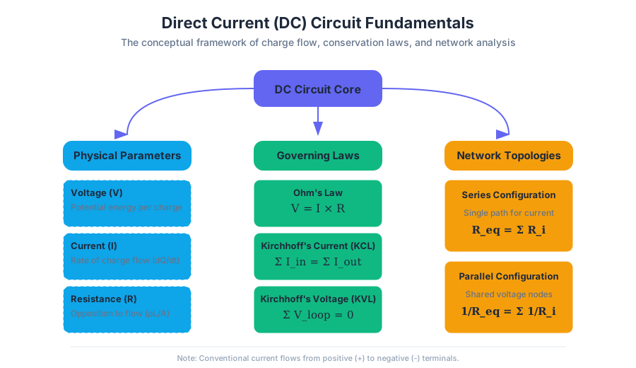
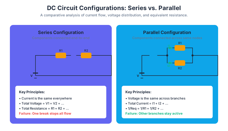
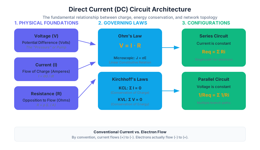
Course Challenge and Mastery
Key concepts: Cumulative Review · Mastery Points · Problem Solving
A final cumulative assessment covering all units of the High School Physics curriculum.
Course Challenge and Mastery
The Course Challenge represents the terminal phase of the pedagogical lifecycle within a technical curriculum. It is not merely a "final exam" in the traditional sense; rather, it is a high-entropy diagnostic tool designed to evaluate a learner's ability to synthesize disparate concepts into a unified mental model. In the context of a Physics curriculum, this involves transitioning from isolated unit-level proficiency to a state of Global Mastery, where the learner can navigate the intersections of kinematics, dynamics, energy, and electromagnetism without the scaffolding provided by modular instruction.
Achieving "Mastery" requires more than just a high score. It demands a demonstration of retention over time and transferability of skill. The Course Challenge serves as the gatekeeper for Mastery Points, the quantitative metric used to track a learner's progression from "Familiar" to "Proficient" and, ultimately, to "Mastered."
The Mechanics of Mastery Points
Mastery is a dynamic state, not a static achievement. The system utilizes a tiered progression model that rewards consistent performance across multiple attempts. Unlike traditional grading, which often penalizes early failures, a mastery-based system views errors as data points in a convergent learning trajectory.
The Mastery Tier Hierarchy
The progression toward mastery is typically divided into four distinct levels. Each level represents a higher degree of cognitive reliability and a lower probability of "false positive" proficiency.
| Level | State | Description | Point Threshold |
|---|---|---|---|
| L0 | Not Started | The learner has not engaged with the material or has failed initial diagnostics. | 0% |
| L1 | Familiar | The learner can solve basic problems with significant prompting or within a narrow context. | 40-60% |
| L2 | Proficient | The learner demonstrates consistent accuracy in unit-level assessments. | 70-90% |
| L3 | Mastered | The learner successfully completes the Course Challenge, demonstrating synthesis and long-term retention. | 100% |
The Mastery Theorem: A concept is considered "Mastered" only when the learner can successfully apply it in a cumulative, randomized environment (the Course Challenge) after a significant temporal delay from the initial instruction phase.
Cumulative Review: The Spacing and Interleaving Effects
The Course Challenge leverages two primary psychological principles: Spaced Repetition and Interleaving. While unit tests focus on "blocked practice" (solving many problems of the same type), the Course Challenge forces the brain to constantly switch between different physical laws and mathematical frameworks.
Blocked vs. Interleaved Practice
| Feature | Blocked Practice (Unit Test) | Interleaved Practice (Course Challenge) |
|---|---|---|
| Context Switching | Low | High |
| Problem Identification | Obvious (based on current unit) | Difficult (must determine which law applies) |
| Long-term Retention | Lower | Significantly Higher |
| Cognitive Load | Moderate | High (Simulates real-world engineering) |
In a Course Challenge, a question on Linear Momentum might be immediately followed by a question on DC Circuits. This "contextual interference" forces the learner to retrieve information from long-term memory more aggressively, strengthening the neural pathways associated with that knowledge.
Synthesis-Level Problem Solving
The hallmark of a senior-level understanding is the ability to solve Synthesis Problems. These are problems where the solution to one part of the problem (e.g., finding velocity using the Work-Energy Theorem) serves as the input for another part of the problem (e.g., using that velocity to calculate the centripetal force in a magnetic field).
The Synthesis Pipeline
- Deconstruction: Identify all physical constants and variables provided.
- Domain Mapping: Determine which domains of physics are involved (e.g., "This is a Kinematics problem disguised as an Energy problem").
- Variable Bridging: Identify the "bridge variable"—the value that connects two different formulas.
- Execution: Perform the algebraic or numerical computation.
- Validation: Check units and order-of-magnitude feasibility.
Worked Example: The Ballistic Pendulum Synthesis
Consider a projectile of mass $m$ moving at velocity $v$ that embeds itself into a stationary pendulum bob of mass $M$. To find the maximum height $h$ reached by the pendulum, the learner must synthesize Conservation of Momentum (the collision) and Conservation of Energy (the swing).
# Low-level implementation of a Ballistic Pendulum Simulation
# Purpose: Calculate the final height of a pendulum after an inelastic collision.

import math

def calculate_pendulum_height(m_projectile, v_projectile, m_bob, g=9.81):
    """
    Synthesizes Linear Momentum and Gravitational Potential Energy.

    Step 1: Conservation of Momentum (Inelastic Collision)
    m*v + M*0 = (m + M) * V_final
    V_final = (m * v) / (m + M)
    """
    total_mass = m_projectile + m_bob
    v_final_system = (m_projectile * v_projectile) / total_mass

    """
    Step 2: Conservation of Energy
    0.5 * (m + M) * V_final^2 = (m + M) * g * h
    h = V_final^2 / (2 * g)
    """
    height = (v_final_system ** 2) / (2 * g)

    return {
        "system_velocity_post_collision": v_final_system,
        "max_height_meters": height,
        "energy_lost_joules": (0.5 * m_projectile * v_projectile**2) - (0.5 * total_mass * v_final_system**2)
    }

# Example Usage: 0.01kg bullet at 400m/s hitting a 2kg bob
result = calculate_pendulum_height(0.01, 400, 2.0)
print(f"Max Height: {result['max_height_meters']:.4f}m")
Technical Prerequisites: The "Client Challenge"
A significant, yet often overlooked, aspect of the Course Challenge is the technical environment in which it is delivered. As noted in the system requirements, the Client Challenge—the browser-side execution of the exam—is heavily dependent on JavaScript (JS).
The Course Challenge is not a static document; it is a dynamic application that handles:
- State Management: Tracking which of the 30 questions have been answered.
- Real-time Validation: Checking answers against an encrypted solution key.
- LaTeX Rendering: Using libraries like MathJax or KaTeX to display complex formulas.
- Interactive Diagrams: SVG-based force diagrams that update based on user input.
The JavaScript Dependency
If JavaScript is disabled, the "Client Challenge" fails because the browser cannot execute the logic required to render the DOM (Document Object Model) elements associated with the exam. This is a critical "Access Requirement" for any modern mastery-based platform.
// A conceptual representation of the Client Challenge initialization
// This script checks for environment readiness before loading the exam.

async function initializeCourseChallenge() {
    const requirements = {
        jsEnabled: true,
        mathJaxLoaded: typeof MathJax !== 'undefined',
        userAuthenticated: checkAuthStatus(),
        browserCompatible: navigator.cookieEnabled
    };

    for (const [key, met] of Object.entries(requirements)) {
        if (!met) {
            console.error(`Critical Error: ${key} requirement not met.`);
            displayErrorMessage(`Please enable ${key} to proceed with the Course Challenge.`);
            return false;
        }
    }

    try {
        const examData = await fetchExamData('/api/v1/course-challenge/physics-high-school');
        renderExamInterface(examData);
        startTimer();
    } catch (err) {
        handleNetworkError(err);
    }
}
Domain Deep Dive: Core Physics Concepts Tested
The Course Challenge tests several key domains. Mastery is achieved when the learner can navigate the specific mathematical nuances of each.
1. Kinematics and One-Dimensional Motion
The foundation of mechanics. It focuses on describing motion without regard to its causes.
- Key Equations: The "Big Four" kinematic equations.
- Common Pitfall: Misinterpreting the sign of acceleration in free-fall (e.g., forgetting that $g$ is downward even when an object is moving upward).
2. Dynamics and Newton’s Laws
The study of forces.
- Newton’s Second Law: $\sum F = ma$.
- Mastery Requirement: Proficiency in drawing Free-Body Diagrams (FBDs) for inclined planes and multi-body systems (Atwood machines).
3. Work, Energy, and Power
The scalar approach to mechanics.
- Work-Energy Theorem: $W_{net} = \Delta K$.
- The Power Formula: $P = \frac{dW}{dt} = \vec{F} \cdot \vec{v}$.
4. Linear Momentum and Collisions
The study of impulse and conservation.
- Elastic vs. Inelastic: In elastic collisions, both momentum and kinetic energy are conserved. In inelastic collisions, only momentum is conserved.
5. Static Electricity and DC Circuits
The transition from mechanics to electromagnetism.
- Coulomb's Law: $F = k \frac{q_1 q_2}{r^2}$.
- Ohm's Law: $V = IR$.
Advanced Problem Archetypes
To reach the "Mastery" level, students must be prepared for specific exam patterns that combine these domains.
| Archetype | Concepts Combined | Difficulty | Logic Flow |
|---|---|---|---|
| The Loop-the-Loop | Energy + Centripetal Force | High | Use $mgh$ to find $v$ at the top, then use $F_c = \frac{mv^2}{r}$ to find Normal Force. |
| The Charged Projectile | Kinematics + Electrostatics | Extreme | Use $E = \frac{F}{q}$ to find acceleration, then apply kinematic equations for trajectory. |
| The Frictional Slide | Dynamics + Energy | Medium | Use $\mu_k F_n$ to find work done by friction, then subtract from initial $E_p$. |
| The Power Lifter | Work + Power + Kinematics | Medium | Calculate Work ($Fd$), then divide by time to find Power. |
Mathematical Derivations for Mastery
A senior engineer or physicist doesn't just memorize formulas; they understand the derivation. The Course Challenge often tests this by asking for variables in terms of other constants.
Derivation of the Work-Energy Theorem
The relationship between work and kinetic energy is derived from Newton's Second Law and the kinematic equation for displacement.
\begin{aligned}
1. & \quad F = ma \\
2. & \quad v_f^2 = v_i^2 + 2a\Delta x \implies a = \frac{v_f^2 - v_i^2}{2\Delta x} \\
3. & \quad W = F \Delta x \\
4. & \quad W = (m \cdot \frac{v_f^2 - v_i^2}{2\Delta x}) \cdot \Delta x \\
5. & \quad W = \frac{1}{2}mv_f^2 - \frac{1}{2}mv_i^2 \\
6. & \quad W = \Delta K
\end{aligned}
Mastery Data Management
From a systems perspective, tracking mastery across thousands of students requires a robust data schema. Each "Mastery Point" is a record in a relational database that tracks the relationship between a student, a specific learning objective, and their performance history.
-- Schema for tracking Mastery Points and Course Challenge attempts
CREATE TABLE student_mastery (
    student_id UUID REFERENCES students(id),
    topic_id VARCHAR(255), -- e.g., 'kinematics_free_fall'
    mastery_points INT DEFAULT 0,
    proficiency_level ENUM('L0', 'L1', 'L2', 'L3'),
    last_attempt_timestamp TIMESTAMP,
    PRIMARY KEY (student_id, topic_id)
);

CREATE TABLE course_challenge_results (
    attempt_id SERIAL PRIMARY KEY,
    student_id UUID REFERENCES students(id),
    score_percentage DECIMAL(5, 2),
    correct_answers INT,
    total_questions INT DEFAULT 30,
    completion_time_seconds INT,
    timestamp TIMESTAMP DEFAULT CURRENT_TIMESTAMP
);

-- Query to identify topics requiring review before the next Course Challenge
SELECT topic_id, mastery_points
FROM student_mastery
WHERE student_id = 'user_123' AND mastery_points < 80;
Common Pitfalls in the Course Challenge
Even high-performing students encounter "edge case" errors that prevent them from achieving full mastery points.
- Vector Directionality: In two-dimensional motion (projectiles), failing to decompose vectors into $x$ and $y$ components.
- Unit Mismatches: Mixing grams with kilograms or centimeters with meters. The system expects SI units unless otherwise specified.
- Static vs. Kinetic Friction: Using $\mu_s$ when the object is already in motion, or failing to check if the applied force exceeds the maximum static friction threshold.
- Energy Dissipation: Forgetting that mechanical energy is not conserved when non-conservative forces (friction, air resistance) are present.
- Rounding Errors: Carrying rounded values through a multi-step calculation. Always keep intermediate values in your calculator's memory.
Summary of Mastery Strategy
Achieving mastery is a marathon, not a sprint. The Course Challenge is the final validation of a journey that begins with basic conceptual understanding. To succeed:
- Enable JavaScript: Ensure your technical environment is ready for the "Client Challenge."
- Practice Synthesis: Don't just solve unit-specific problems; look for "bridge" problems.
- Review FBDs: Dynamics is the "engine" of physics; if you can't draw the forces, you can't solve the motion.
- Embrace the Interleave: If the Course Challenge feels harder than the unit tests, it's working. That struggle is the sound of your brain building a more resilient model of the universe.
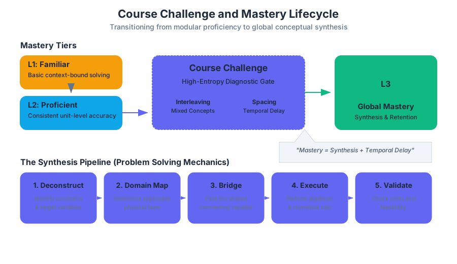

Source Materials
Study High School Physics with AI — Free on Lykke
Sign up for free to generate personalized flashcards, quizzes, and study guides from this course. Chat with an AI tutor that knows the material.
Get Started FreeView this course wiki on Lykke · Browse all public course wikis