High School Chemistry
Institution: MIT
42 study materials · 9 sections
The Client Challenge course is a comprehensive High School Chemistry curriculum meticulously aligned with the Next Generation Science Standards (NGSS). It guides students through eleven core units, beginning with the fundamental building blocks of matter—atoms, isotopes, and ions—and advancing toward complex topics like stoichiometry, thermodynamics, and nuclear chemistry. The course emphasizes the transition from classical atomic models to modern quantum mechanics, providing a robust framework for understanding chemical bonding and periodic trends.
Course Sections
Fundamental Building Blocks: Atoms, Isotopes, and Ions
Key concepts: Protons, neutrons, and electrons · Isotopes and average atomic mass · Cations and anions · Lewis diagrams
An introduction to subatomic particles, the identification of isotopes, and the formation of charged ions.
Fundamental Building Blocks: Atoms, Isotopes, and Ions
Overview
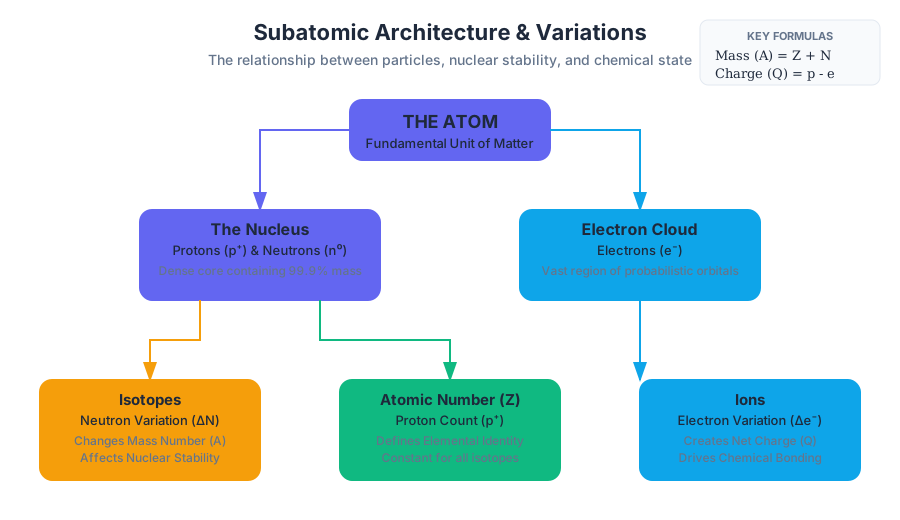
In the study of chemistry, we often treat the atom as the fundamental unit of matter. However, to understand the macroscopic behavior of substances—why sodium explodes in water, why carbon forms the backbone of life, or why certain isotopes are radioactive—we must peer into the subatomic architecture. The properties of matter are not arbitrary; they are the emergent consequences of the arrangement and quantity of three primary subatomic particles: protons, neutrons, and electrons.
This section explores the internal structure of the atom, the variations in nuclear composition known as isotopes, the electrostatic imbalances that create ions, and the symbolic language of Lewis diagrams used to predict chemical reactivity.
The Architecture of the Atom
At its most basic level, an atom is an organized collection of subatomic particles. While modern quantum mechanics describes these particles as wave-functions with probabilistic locations, the "Solar System" or Bohr-inspired model remains a highly effective pedagogical tool for understanding chemical identity and stoichiometry.
The Subatomic Trinity: Protons, Neutrons, and Electrons
The atom is divided into two distinct regions: the nucleus and the electron cloud.
- The Nucleus: A dense, positively charged core containing protons and neutrons (collectively called nucleons). Despite occupying less than 0.01% of the atom's volume, the nucleus contains over 99.9% of its mass.
- The Electron Cloud: A vast, mostly empty region surrounding the nucleus where electrons reside in specific energy levels or orbitals.
| Particle | Symbol | Charge (e) | Mass (amu) | Mass (kg) | Location |
|---|---|---|---|---|---|
| Proton | $p^+$ | +1 | 1.00727 | $1.672 \times 10^{-27}$ | Nucleus |
| Neutron | $n^0$ | 0 | 1.00866 | $1.674 \times 10^{-27}$ | Nucleus |
| Electron | $e^-$ | -1 | 0.00055 | $9.109 \times 10^{-31}$ | Orbitals |
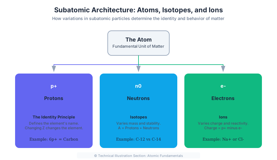
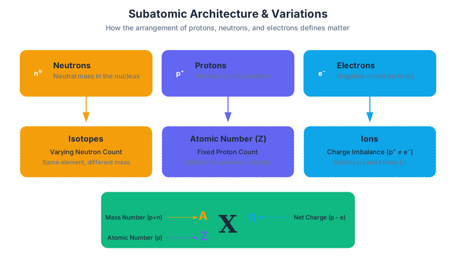
The Identity Principle: The number of protons in the nucleus, known as the Atomic Number ($Z$), uniquely defines the element. If you change the number of protons, you change the element itself. For example, any atom with exactly 6 protons is Carbon, regardless of its neutron or electron count.
Mathematical Representation of Atomic State
To programmatically represent an atom's fundamental state, we can define a structure that tracks these three variables. In a computational chemistry context, an atom's state is the baseline for all further simulations.
class Atom:
    """
    A class representing the fundamental state of an atom.
    Calculates identity, mass number, and net charge.
    """
    def __init__(self, protons, neutrons, electrons):
        self.z = protons         # Atomic Number
        self.n = neutrons        # Neutron Number
        self.e = electrons       # Electron Number

        # Periodic Table Mapping (Simplified)
        self.elements = {1: "H", 6: "C", 7: "N", 8: "O", 11: "Na", 17: "Cl"}

    @property
    def mass_number(self):
        # A = Z + N
        return self.z + self.n

    @property
    def net_charge(self):
        # Charge = Protons - Electrons
        return self.z - self.e

    def get_notation(self):
        symbol = self.elements.get(self.z, "??")
        charge_str = f"{self.net_charge:+}" if self.net_charge != 0 else ""
        return f"[{self.mass_number} / {self.z}] {symbol} {charge_str}"

# Example: Carbon-14 Anion (hypothetical for demonstration)
c14 = Atom(protons=6, neutrons=8, electrons=7)
print(f"Nuclide: {c14.get_notation()}")
# Output: Nuclide: [14 / 6] C -1
Isotopes and the Nuclide Landscape
While the number of protons defines the element, the number of neutrons can vary. These variations are called isotopes.
Defining Isotopes
Isotopes are atoms of the same element (same $Z$) that possess different numbers of neutrons ($N$), resulting in different Mass Numbers ($A$).
Theorem of Isotopic Identity: For any element $X$, isotopes exist as $^A_Z X$, where $Z$ is constant and $A$ varies.
Why Isotopes Matter: Stability and Mass
Neutrons act as the "nuclear glue." Because protons are all positively charged, they exert a powerful electrostatic repulsion against one another. The Strong Nuclear Force, mediated by neutrons, overcomes this repulsion to keep the nucleus intact.
- If there are too few neutrons, the repulsion wins and the nucleus flies apart.
- If there are too many, the nucleus becomes unstable. This instability leads to radioactivity, a core concept in nuclear chemistry and medical imaging.
Calculating Average Atomic Mass
The mass listed on the periodic table (e.g., 35.45 for Chlorine) is not the mass of a single atom. It is the Average Atomic Mass, a weighted average of all naturally occurring isotopes of that element.
\text{Average Atomic Mass} = \sum_{i=1}^{n} (\text{Mass of Isotope}_i \times \text{Abundance}_i)
Worked Example: Chlorine Chlorine has two stable isotopes:
- $^{35}\text{Cl}$: Mass $\approx 34.969$ amu, Abundance $\approx 75.77%$
- $^{37}\text{Cl}$: Mass $\approx 36.966$ amu, Abundance $\approx 24.23%$
Calculation: $(34.969 \times 0.7577) + (36.966 \times 0.2423) = 26.496 + 8.957 = 35.453 \text{ amu}$
| Isotope | Protons | Neutrons | Mass (amu) | Natural Abundance |
|---|---|---|---|---|
| Protium ($^1\text{H}$) | 1 | 0 | 1.0078 | 99.98% |
| Deuterium ($^2\text{H}$) | 1 | 1 | 2.0141 | 0.015% |
| Tritium ($^3\text{H}$) | 1 | 2 | 3.0160 | Trace (Radioactive) |
Ions: The Drivers of Chemical Reactivity
In a neutral atom, the number of protons equals the number of electrons. However, atoms are often "unhappy" in this state. Stability in chemistry is frequently governed by the Octet Rule, where atoms seek to have a full outer shell of electrons (typically eight). To achieve this, atoms will either gain or lose electrons, becoming ions.
Cations: The Electron Losers
Cations are positively charged ions formed when an atom loses one or more electrons. This typically happens to metals (Groups 1, 2, and 13), which have few valence electrons and find it energetically "cheaper" to shed them.
- Example: Sodium ($\text{Na}$) has 11 electrons. Its configuration is $[2, 8, 1]$. By losing 1 electron, it becomes $\text{Na}^+$, achieving the stable configuration of Neon $[2, 8]$.
Anions: The Electron Gainers
Anions are negatively charged ions formed when an atom gains electrons. This typically occurs with non-metals (Groups 15, 16, and 17), which are close to completing their octet.
- Example: Chlorine ($\text{Cl}$) has 17 electrons $[2, 8, 7]$. By gaining 1 electron, it becomes $\text{Cl}^-$, achieving the stable configuration of Argon $[2, 8, 8]$.
The Electrostatic Motivation: The formation of ions is driven by the search for the lowest energy state. The energy required to remove an electron is the Ionization Energy, while the energy released when adding an electron is Electron Affinity.
Comparison of Ion Types
| Feature | Cation | Anion |
|---|---|---|
| Charge | Positive ($+$) | Negative ($-$) |
| Formation | Loss of electrons | Gain of electrons |
| Typical Elements | Metals | Non-metals |
| Atomic Radius | Smaller than parent atom | Larger than parent atom |
| Naming | Element name + "ion" (e.g., Sodium ion) | Element root + "-ide" (e.g., Chloride) |
Technical Representation: Ion Data Structures
In database schemas or configuration files for chemical simulations, ions are often defined by their oxidation states and coordination numbers.
{
  "ion_registry": [
    {
      "element": "Magnesium",
      "symbol": "Mg",
      "common_charge": +2,
      "type": "cation",
      "electron_configuration_change": "-2e",
      "radius_change_pm": -65
    },
    {
      "element": "Oxygen",
      "symbol": "O",
      "common_charge": -2,
      "type": "anion",
      "electron_configuration_change": "+2e",
      "radius_change_pm": +70
    }
  ]
}
Lewis Diagrams: Mapping the Valence Shell
As we move toward understanding chemical bonding, we need a way to visualize the electrons that actually participate in reactions: the valence electrons. Lewis Diagrams (or Lewis Dot Structures) provide a shorthand for this.
The Mechanics of Lewis Dots
A Lewis diagram consists of the element's chemical symbol surrounded by dots representing its valence electrons.
- Identify the Group Number: For main-group elements, the number of valence electrons corresponds to the ones digit of their group number (e.g., Group 14 has 4 valence electrons).
- Place Dots Singly: Following Hund's Rule logic, place one dot on each of the four sides (top, bottom, left, right) before pairing them up.
- Maximum of Eight: Since the valence shell (s and p orbitals) holds a maximum of 8 electrons, no more than 8 dots are shown.
Lewis Diagrams for Ions
When drawing ions:
- Cations: Usually have no dots shown (since they lost their valence shell) and are enclosed in brackets with the charge outside.
- Anions: Usually have a full set of 8 dots and are enclosed in brackets with the charge outside.
| Group | Valence $e^-$ | Lewis Pattern Example |
|---|---|---|
| 1 (Alkali) | 1 | $\text{Li} \cdot$ |
| 2 (Alkaline Earth) | 2 | $\cdot \text{Be} \cdot$ |
| 13 (Boron) | 3 | 3 single dots |
| 14 (Carbon) | 4 | 4 single dots |
| 17 (Halogens) | 7 | 3 pairs, 1 single |
| 18 (Noble Gases) | 8 | 4 pairs (Full Octet) |
Implementation: A Low-Level View of Electron States
In a systems-level simulation (e.g., written in Rust), we might represent the valence state as a bitfield to optimize for speed in bonding calculations.
/// Represents the valence shell of an atom using a bitfield.
/// Each bit represents an electron slot in the s and p orbitals.
struct ValenceShell {
    // 00000000 to 11111111 (8 bits for the octet)
    bits: u8,
}

impl ValenceShell {
    fn new(count: u8) -> Self {
        // Fill bits from right to left based on electron count
        let mut bits = 0u8;
        for i in 0..count {
            bits |= 1 << i;
        }
        ValenceShell { bits }
    }

    fn is_full(&self) -> bool {
        self.bits == 0xFF // 255 in decimal, all 8 bits set
    }

    fn count_unpaired(&self) -> u8 {
        // Simplified logic for Lewis dot pairing
        // In reality, electrons pair after 4 single slots are filled
        let count = self.bits.count_ones();
        if count <= 4 { count as u8 } else { (8 - count) as u8 }
    }
}
Common Pitfalls and Misconceptions
- Mass vs. Weight: Students often confuse "Mass Number" (an integer: $p + n$) with "Atomic Mass" (a decimal average). Remember: an individual atom never has a mass of 35.45 amu; it is either 35 or 37.
- The Electron's Mass: While we often say electrons have "no mass," they actually have about 1/1836th the mass of a proton. In high-precision mass spectrometry, this difference matters.
- Charge Sign Confusion: A common error is thinking that adding electrons makes an atom positive. Remember: Electrons are negative. Adding them increases negativity (Anion); removing them increases positivity (Cation).
- The Nucleus is Not Static: While we treat $Z$ as fixed in chemistry, in nuclear physics, $Z$ can change through beta decay, effectively turning one element into another (transmutation).
Summary
The atom is a balance of forces. The number of protons determines the "soul" of the atom (its element), the neutrons determine its "heaviness" and stability (its isotope), and the electrons determine its "personality" and social life (its ions and bonding). By mastering these building blocks, we gain the ability to predict the behavior of every substance in the known universe.
Modern Atomic Theory and Periodicity
Key concepts: Bohr model · Quantum mechanical model · Electron configurations · Periodic table organization · Atomic spectra
Exploration of the transition from the Bohr model to the quantum mechanical model and how these theories explain periodic trends.
Modern Atomic Theory and Periodicity
The transition from a classical understanding of the atom to the modern quantum mechanical model represents one of the most significant paradigm shifts in scientific history. While the early 20th century viewed atoms as miniature solar systems, we now understand them as complex wave-functions governed by probability and quantization. This article explores the mechanics of the atom, the mathematical underpinnings of electron behavior, and how these microscopic properties manifest as the macroscopic patterns of the Periodic Table.
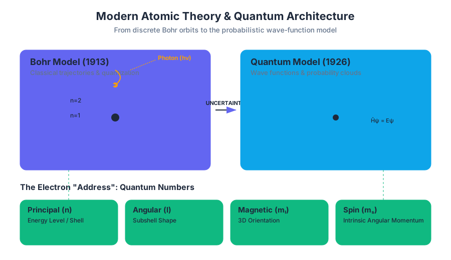
The Bohr Model and the Birth of Quantization
Before the advent of full quantum mechanics, Niels Bohr proposed a model in 1913 that bridged the gap between classical physics and the emerging evidence of energy quantization. Bohr’s model was a direct response to the "ultraviolet catastrophe" and the observed discrete lines in atomic spectra.
The Mechanics of the Bohr Atom
Bohr postulated that electrons travel in defined circular orbits around the nucleus. Unlike a planet orbiting a sun, which can exist at any distance, an electron can only occupy specific, quantized energy levels.
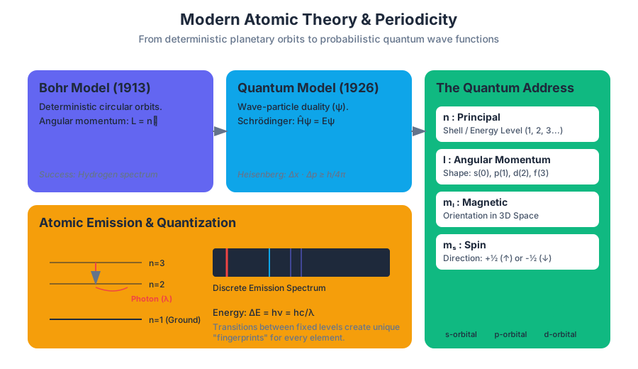
Bohr’s Postulate: The angular momentum of an electron is quantized in integral multiples of $\hbar$ (h-bar), expressed as $L = n\hbar$, where $n$ is the principal quantum number.
Atomic Spectra and Energy Transitions
When an atom absorbs energy (via heat or electricity), an electron is promoted from a ground state to an excited state. When it falls back to a lower energy level, it releases a photon with an energy exactly equal to the difference between the two levels. This is why elements produce distinct spectral lines rather than a continuous rainbow.
The energy of the emitted photon is calculated using the Planck-Einstein relation: $$E = h\nu = \frac{hc}{\lambda}$$
Where:
- $h$ is Planck's constant ($6.626 \times 10^{-34} \text{ J}\cdot\text{s}$)
- $\nu$ is frequency
- $c$ is the speed of light
- $\lambda$ is wavelength
Worked Example: The Rydberg Formula
To calculate the wavelength of light emitted during an electronic transition in a hydrogen atom, we use the Rydberg formula:
import numpy as np

def calculate_rydberg_wavelength(n_final, n_initial):
    """
    Calculates the wavelength (in meters) of light emitted
    during a hydrogen electron transition.

    Formula: 1/λ = R_H * (1/n_f² - 1/n_i²)
    R_H (Rydberg constant) ≈ 1.097 x 10^7 m⁻¹
    """
    R_H = 1.0973731568e7

    if n_initial <= n_final:
        raise ValueError("n_initial must be greater than n_final for emission.")

    inv_lambda = R_H * ( (1 / n_final**2) - (1 / n_initial**2) )
    wavelength = 1 / inv_lambda

    return wavelength

# Example: Transition from n=3 to n=2 (H-alpha line)
wavelength_m = calculate_rydberg_wavelength(2, 3)
print(f"Wavelength: {wavelength_m * 1e9:.2f} nm")
# Output: 656.11 nm (Visible Red Light)
| Feature | Bohr Model | Quantum Mechanical Model |
|---|---|---|
| Electron Path | Defined circular orbits | Probability distributions (orbitals) |
| Certainty | Position and momentum known | Heisenberg Uncertainty Principle applies |
| Energy Levels | Defined by $n$ only | Defined by $n, l, m_l$ |
| Success | Excellent for Hydrogen | Accurate for all elements |
The Quantum Mechanical Model
The Bohr model failed for atoms with more than one electron because it could not account for electron-electron repulsions or the wave-like nature of matter. In 1926, Erwin Schrödinger formulated the wave equation, treating the electron not as a particle, but as a wave function ($\psi$).
The Schrödinger Equation
The fundamental equation of quantum mechanics describes the evolution of a quantum system. For a non-relativistic electron in an atom, the time-independent Schrödinger equation is:
\hat{H}\psi = E\psi
Where:
- $\hat{H}$ is the Hamiltonian operator (representing the sum of kinetic and potential energy).
- $\psi$ (psi) is the wave function.
- $E$ is the energy of the state.
The square of the wave function, $|\psi|^2$, represents the probability density—the likelihood of finding an electron in a specific region of space. This region is what we call an orbital.
The Heisenberg Uncertainty Principle
A cornerstone of the quantum model is the realization that we cannot simultaneously know the exact position ($x$) and momentum ($p$) of a particle.
Heisenberg Uncertainty Principle: $\Delta x \cdot \Delta p \ge \frac{h}{4\pi}$
This principle effectively "smears" the electron into a cloud, replacing Bohr's trajectories with orbital volumes.
Quantum Numbers and Orbital Architecture
To describe the "address" of an electron within an atom, we use four quantum numbers. These numbers emerge naturally from the solutions to the Schrödinger equation.
1. Principal Quantum Number ($n$)
Indicates the main energy level or shell. As $n$ increases, the orbital becomes larger and the electron spends more time further from the nucleus.
- Values: $n = 1, 2, 3, \dots$
2. Angular Momentum Quantum Number ($l$)
Defines the shape of the orbital (subshell).
- Values: $0$ to $(n-1)$
- Mapping: $0=s, 1=p, 2=d, 3=f$
3. Magnetic Quantum Number ($m_l$)
Defines the orientation of the orbital in 3D space.
- Values: $-l$ to $+l$
4. Spin Quantum Number ($m_s$)
Describes the intrinsic angular momentum (spin) of the electron.
- Values: $+1/2$ (spin up) or $-1/2$ (spin down)
| Subshell ($l$) | Shape | Number of Orbitals | Max Electrons |
|---|---|---|---|
| s (0) | Spherical | 1 | 2 |
| p (1) | Dumbbell | 3 | 6 |
| d (2) | Cloverleaf/Complex | 5 | 10 |
| f (3) | Complex | 7 | 14 |
Electron Configurations: The Aufbau Process
Electron configuration is the distribution of electrons among the various orbitals. The "filling" of these orbitals follows three strict principles:
- Aufbau Principle: Electrons occupy the lowest energy orbitals first (e.g., 1s before 2s).
- Pauli Exclusion Principle: No two electrons in an atom can have the same four quantum numbers. Therefore, an orbital can hold a maximum of two electrons with opposite spins.
- Hund’s Rule: For degenerate orbitals (orbitals with the same energy, like the three 2p orbitals), electrons fill them singly first with parallel spins before pairing up.
The Madelung Rule (n + l Rule)
The order of filling is generally determined by the sum of $n + l$. If two orbitals have the same $n + l$, the one with the lower $n$ is filled first.
# Order of orbital filling (The Diagonal Rule)
1s -> 2s -> 2p -> 3s -> 3p -> 4s -> 3d -> 4p -> 5s -> 4d -> 5p -> 6s ...
Noble Gas Notation
To simplify configurations for heavy elements, we use the previous noble gas as a "core" shortcut.
- Sodium (Na): $1s^2 2s^2 2p^6 3s^1 \rightarrow [Ne] 3s^1$
- Iron (Fe): $1s^2 2s^2 2p^6 3s^2 3p^6 4s^2 3d^6 \rightarrow [Ar] 4s^2 3d^6$
Exceptions to the Rule
Transition metals like Chromium (Cr) and Copper (Cu) deviate from the standard Aufbau order to achieve the stability of half-filled or fully-filled d-subshells.
- Cr expected: $[Ar] 4s^2 3d^4$
- Cr actual: $[Ar] 4s^1 3d^5$ (Half-filled stability)
Periodicity and the Organization of the Table
The Periodic Table is not merely a list; it is a map of electron configurations. The layout is divided into blocks ($s, p, d, f$) corresponding to the subshell being filled in the valence shell.
Effective Nuclear Charge ($Z_{eff}$)
The core concept driving periodic trends is Effective Nuclear Charge. While the nucleus has a positive charge ($Z$), the inner-shell electrons "shield" the outer electrons from the full pull of the nucleus.
Formula: $Z_{eff} = Z - S$ Where $Z$ is the atomic number and $S$ is the screening constant (number of core electrons).
Periodic Trends Summary
| Trend | Definition | Direction (Across Period) | Direction (Down Group) |
|---|---|---|---|
| Atomic Radius | Distance from nucleus to valence shell | Decreases (higher $Z_{eff}$ pulls tighter) | Increases (more shells) |
| Ionization Energy | Energy required to remove an electron | Increases (stronger nuclear pull) | Decreases (further from nucleus) |
| Electronegativity | Ability to attract electrons in a bond | Increases (except Noble Gases) | Decreases |
| Electron Affinity | Energy change when an electron is added | Becomes more negative (generally) | Becomes less negative |
Deep Dive: Ionization Energy ($IE$)
Ionization energy provides a direct measurement of how tightly an atom holds its electrons. Successive ionization energies ($IE_1, IE_2, IE_3$) show massive jumps when an electron is removed from a core shell.
Example: Magnesium (Mg)
- $IE_1$: 738 kJ/mol (Remove $3s^1$)
- $IE_2$: 1451 kJ/mol (Remove $3s^2$)
- $IE_3$: 7733 kJ/mol (Remove $2p^6$ — Huge Jump!)
The jump at $IE_3$ confirms that Magnesium has two valence electrons.
Real-World Application: Computational Chemistry
Modern chemical engineering relies on simulating these configurations to predict material properties. Using libraries like mendeleev, engineers can programmatically access these periodic properties for high-throughput screening.
from mendeleev import element

def analyze_element_stability(symbol):
    el = element(symbol)

    print(f"Element: {el.name} ({el.symbol})")
    print(f"Atomic Number: {el.atomic_number}")
    print(f"Electronic Configuration: {el.ec.conf}")
    print(f"First Ionization Energy: {el.ionenergies[1]} eV")

    # Check for valence shell status
    valence_electrons = el.nvalence()
    print(f"Valence Electrons: {valence_electrons}")

    if valence_electrons == 8 or (el.symbol == 'He' and valence_electrons == 2):
        print("Status: Highly stable (Noble Gas configuration)")
    else:
        print("Status: Chemically reactive")

analyze_element_stability('Ar')
# Output: Element: Argon (Ar)... Valence Electrons: 8... Highly stable
Common Pitfalls and Misconceptions
- The "Solar System" Fallacy: Students often visualize electrons moving in tracks. In reality, an electron is "everywhere and nowhere" within its orbital until measured.
- 4s vs 3d Energy: While 4s fills before 3d (Aufbau), once the 3d subshell begins to fill, the energy levels shift. When transition metals form ions, they typically lose 4s electrons before 3d electrons.
- Atomic Radius and $Z$: It is counter-intuitive that adding more protons and electrons (moving right across a period) makes the atom smaller. This happens because the increased $Z_{eff}$ pulls the electron cloud closer, and no new shells are added to counteract the pull.
Summary of Modern Atomic Theory
The modern atom is a balance of electrostatic forces and quantum probabilities. The nucleus provides the central potential, while the electrons arrange themselves into quantized states that minimize energy and maximize stability. This arrangement—the electron configuration—is the fundamental "source code" of the universe, dictating how every element bonds, reacts, and exists.
- Bohr Model: A model of the atom where electrons occupy fixed circular orbits with quantized energy.
- Orbital: A mathematical function describing the 3D region where there is a high probability of finding an electron.
- Aufbau Principle: The rule stating that electrons fill the lowest-energy orbitals first.
- Effective Nuclear Charge ($Z_{eff}$): The net positive charge experienced by an electron in a multi-electron atom.
- Ionization Energy: The minimum energy required to remove an electron from a gaseous atom or ion.
- Degenerate Orbitals: Orbitals that have the same energy level (e.g., the three $p$ orbitals in a single shell).
- Heisenberg Uncertainty Principle: The fundamental limit to the precision with which certain pairs of physical properties, such as position and momentum, can be known.
-
Why does the atomic radius decrease as you move from left to right across a period?
- A) The number of energy shells increases.
- B) The effective nuclear charge increases, pulling electrons closer.
- C) Electrons repel each other more strongly.
- D) The mass of the nucleus decreases. (Correct: B)
-
Which quantum number determines the shape of an orbital?
- A) $n$
- B) $l$
- C) $m_l$
- D) $m_s$ (Correct: B)
-
What is the correct noble gas configuration for Sulfur (S, Atomic No. 16)?
- A) $[Ne] 3s^2 3p^4$
- B) $[Ar] 3s^2 3p^4$
- C) $[Ne] 3s^2 3p^6$
- D) $[He] 2s^2 2p^6 3s^2 3p^4$ (Correct: A)
-
According to Hund's Rule, how are electrons placed in degenerate orbitals?
- A) They pair up immediately to minimize space.
- B) They fill the highest energy orbital first.
- C) They fill each orbital singly with parallel spins before pairing.
- D) They are placed randomly. (Correct: C)
-
A transition from $n=4$ to $n=2$ in a hydrogen atom emits light. Compared to a transition from $n=3$ to $n=2$, the emitted light will have:
- A) Longer wavelength, lower energy.
- B) Shorter wavelength, higher energy.
- C) The same wavelength.
- D) No color (infrared). (Correct: B)
Mastery Checklist:
- Derive the energy of a photon given its wavelength.
- Explain why the Bohr model is considered "semi-classical."
- Write the full and condensed electron configurations for any element up to $Z=54$.
- Identify the four quantum numbers for the valence electron of Potassium.
- Predict the relative ionization energy of two elements based on their position in the Periodic Table.
- Explain the "jump" in successive ionization energies for Group 2 vs Group 13 elements.
- Describe the physical significance of the square of the wave function ($|\psi|^2$).
Chemical Bonding and Molecular Structure
Key concepts: Ionic Bonding · Covalent Bonding · Metallic Bonding · Lewis Structures · Bond Polarity
Detailed study of how atoms and ions interact to form ionic, covalent, and metallic bonds.
Chemical Bonding and Molecular Structure
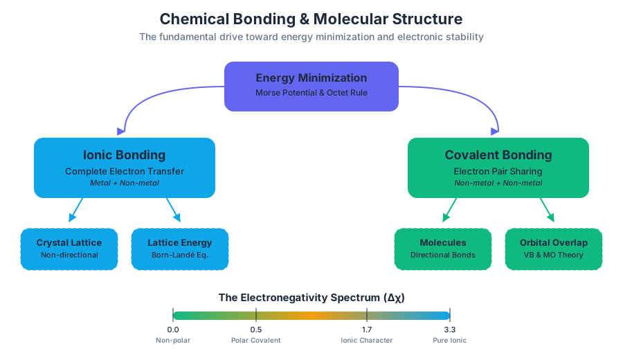
Atoms, in their elemental state, are rarely found in isolation under standard terrestrial conditions. The vast diversity of matter—from the silicon chips in a CPU to the hemoglobin in our blood—is the result of chemical bonding. At its most fundamental level, a chemical bond is a lasting attraction between atoms, ions, or molecules that enables the formation of chemical compounds. This attraction is driven by the universal physical principle of energy minimization: atoms bond because the resulting system has a lower potential energy than the sum of the individual, isolated atoms.
The Energetics of Bonding: Why Atoms Interact
The formation of a bond is governed by the interplay of electrostatic forces: the attraction between nuclei and electrons, and the repulsion between nuclei and between electrons. The Octet Rule serves as a useful heuristic for understanding this behavior, suggesting that atoms are most stable when they possess a full valence shell (typically eight electrons, mimicking the electron configuration of a noble gas).
Mathematically, the stability of a bond can be described by the Morse Potential or the Lennard-Jones Potential, which models the potential energy of a diatomic system as a function of internuclear distance.
Key Insight: The Thermodynamic Drive A chemical bond forms when the change in Gibbs Free Energy ($\Delta G$) for the process is negative. This is primarily achieved through a decrease in enthalpy ($\Delta H$), as the electrostatic attractions release energy when the bond is established.
Ionic Bonding: The Electrostatic Lattice
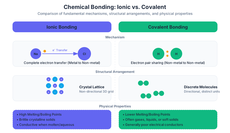
Ionic bonding occurs through the complete transfer of one or more electrons from one atom (typically a metal with low ionization energy) to another (typically a non-metal with high electron affinity). This transfer creates cations (positively charged) and anions (negatively charged), which are then held together by intense Coulombic attraction.
Mechanics of the Ionic Bond
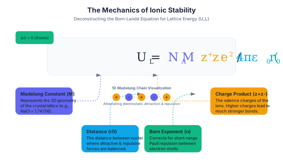
Unlike covalent bonds, ionic bonds are non-directional. A single sodium ion does not "belong" to a single chloride ion; instead, they arrange themselves into a repeating 3D pattern known as a crystal lattice. The strength of this structure is quantified by its Lattice Energy ($U_L$), the energy released when gaseous ions combine to form one mole of an ionic solid.
The Lattice Energy can be approximated using the Born-Landé equation:
U_L = \frac{N_A M z^+ z^- e^2}{4\pi \epsilon_0 r_0} \left( 1 - \frac{1}{n} \right)
Where:
- $N_A$ is Avogadro's constant.
- $M$ is the Madelung constant, representing the geometry of the crystal.
- $z^+, z^-$ are the charges of the ions.
- $e$ is the elementary charge.
- $r_0$ is the equilibrium distance between ions.
- $n$ is the Born exponent.
Properties of Ionic Compounds
| Property | Characteristic | Physical Basis |
|---|---|---|
| Melting/Boiling Point | Very High | Requires breaking strong Coulombic forces throughout the lattice. |
| Brittleness | High | Stress shifts ion layers; like-charges align and repel, shattering the crystal. |
| Electrical Conductivity | Only in molten/aqueous state | Ions must be mobile to carry charge; they are fixed in the solid lattice. |
| Solubility | Often high in polar solvents | Ion-dipole interactions can overcome lattice energy (hydration). |
Worked Example: Calculating Lattice Potential Energy
The following Python script demonstrates how we can programmatically calculate the electrostatic potential energy of a simple linear chain of ions to understand the concept of the Madelung constant.
import numpy as np

def calculate_madelung_linear(num_ions):
    """
    Calculates the Madelung constant for a 1D chain of alternating ions.
    Formula: M = 2 * sum((-1)^(j+1) / j) for j=1 to infinity.
    """
    madelung_sum = 0.0
    for j in range(1, num_ions + 1):
        # Alternating charges: attraction (+), repulsion (-)
        term = ((-1)**(j + 1)) / j
        madelung_sum += term

    # Multiply by 2 for both directions (left and right of the reference ion)
    return 2 * madelung_sum

# Convergence test
for n in [10, 100, 1000, 10000]:
    m = calculate_madelung_linear(n)
    print(f"Ions: {n:5} | Madelung Constant (1D): {m:.6f}")

# The theoretical limit for a 1D chain is 2 * ln(2) ≈ 1.386294
Covalent Bonding: The Shared Electron Model
Covalent bonding involves the sharing of electron pairs between atoms, typically non-metals. This sharing allows each atom to achieve a stable electron configuration. Unlike the electrostatic "clumping" of ionic bonds, covalent bonds are directional and result in the formation of discrete molecules.
Valence Bond Theory vs. Molecular Orbital Theory
- Valence Bond (VB) Theory: Proposes that a bond forms when the atomic orbitals of two atoms overlap. The shared electrons are localized between the two nuclei.
- Molecular Orbital (MO) Theory: Suggests that atomic orbitals combine to form new molecular orbitals that extend over the entire molecule. This explains phenomena like the paramagnetism of $O_2$ which VB theory fails to predict.
Bond Polarity and Electronegativity
Not all sharing is equal. The degree of sharing is determined by Electronegativity ($\chi$), a measure of an atom's ability to attract shared electrons.
- Non-polar Covalent: $\Delta\chi < 0.5$ (Equal sharing, e.g., $H-H$).
- Polar Covalent: $0.5 \le \Delta\chi \le 1.7$ (Unequal sharing, e.g., $H-Cl$).
- Ionic: $\Delta\chi > 1.7$ (Electron transfer, e.g., $Na-Cl$).
Theorem: The Dipole Moment A polar bond creates a bond dipole, quantified by the dipole moment $\mu = Q \times r$, where $Q$ is the partial charge and $r$ is the distance between charges. The net dipole of a molecule is the vector sum of all individual bond dipoles.
Lewis Structures: Mapping the Molecule
Lewis Structures are 2D representations used to visualize the bonding and lone pairs in a molecule. They are essential for predicting molecular geometry via VSEPR theory.
The Algorithm for Drawing Lewis Structures
- Count Valence Electrons: Sum the valence electrons for all atoms. Adjust for charge (add for anions, subtract for cations).
- Identify the Central Atom: Usually the least electronegative atom (never Hydrogen).
- Connect Atoms: Draw single bonds (lines) between the central atom and peripheral atoms.
- Distribute Remaining Electrons: Complete the octets of the peripheral atoms first, then place remaining electrons on the central atom.
- Satisfy the Octet Rule: If the central atom lacks an octet, move lone pairs from peripheral atoms to form double or triple bonds.
Formal Charge Calculation
To determine the most plausible Lewis structure among resonance contributors, we calculate the Formal Charge (FC) for each atom:
FC = [Valence Electrons] - [Non-bonding Electrons] - (1/2)[Bonding Electrons]
The most stable structure is the one where formal charges are closest to zero and negative charges reside on the most electronegative atoms.
Resonance and Exceptions
Some molecules cannot be described by a single Lewis structure. Resonance occurs when multiple valid structures exist; the actual molecule is a hybrid of these forms. Furthermore, some atoms violate the octet rule:
- Incomplete Octets: Boron and Beryllium often form compounds with fewer than 8 electrons (e.g., $BF_3$).
- Expanded Octets: Elements in Period 3 and below can use d-orbitals to hold more than 8 electrons (e.g., $SF_6$, $PCl_5$).
Metallic Bonding: The "Sea of Electrons"
Metallic bonding explains the unique properties of metals. In this model, metal atoms lose their valence electrons to a "delocalized sea" that surrounds a lattice of positive metal cations.
Band Theory
A more advanced view is Band Theory, which treats the delocalized electrons as occupying energy bands.
- Conduction Band: The range of electron energies enough to free an electron from binding with its atom to move freely within the atomic lattice.
- Valence Band: The highest range of electron energies in which electrons are normally present at absolute zero temperature.
- In metals, these bands overlap, allowing for high electrical and thermal conductivity.
Comparison of Bonding Characteristics
| Feature | Ionic | Covalent | Metallic |
|---|---|---|---|
| Bonding Particles | Cations and Anions | Atoms | Cations and Delocalized Electrons |
| Force of Attraction | Electrostatic | Shared electron pairs | Attraction between cations and electron sea |
| State at Room Temp | Solid | Gas, Liquid, or Solid | Solid (except Mercury) |
| Malleability | No (Brittle) | No | Yes |
| Conductivity (Solid) | Low | Low | High |
Common Pitfalls and Misconceptions
- The "Ionic vs. Covalent" Binary: Many students view bonds as either 100% ionic or 100% covalent. In reality, bonding exists on a continuum. Even "ionic" bonds like $Li-F$ have a small degree of covalent character.
- Octet Obsession: The octet rule is a guideline, not a law. Transition metals and heavy non-metals frequently ignore it.
- Geometry Confusion: Lewis structures are 2D. They do not represent the actual 3D shape. For instance, $CH_4$ is drawn as a cross but is actually a tetrahedron ($109.5^\circ$).
- Bond Breaking vs. Phase Change: Boiling water breaks intermolecular forces (Hydrogen bonds), not the intramolecular covalent $O-H$ bonds.
Advanced Representation: Chemical Data Structures
In computational chemistry, molecules are often represented as graphs or strings. The SMILES (Simplified Molecular Input Line Entry System) format is a standard for describing molecular structures in a way that a computer can process.
# Example: Using RDKit (Python library) to process a SMILES string
# Molecule: Aspirin (2-acetoxybenzoic acid)
# SMILES: CC(=O)OC1=CC=CC=C1C(=O)O

# CLI command to generate a 3D structure from SMILES (conceptual)
obabel -:"CC(=O)OC1=CC=CC=C1C(=O)O" -O aspirin.sdf --gen3d
Database Schema for Molecular Storage
When building a chemical database, one must store both the connectivity (bonds) and the properties.
CREATE TABLE molecules (
    molecule_id INT PRIMARY KEY,
    common_name VARCHAR(255),
    iupac_name TEXT,
    smiles_string TEXT UNIQUE,
    molecular_weight DECIMAL(10, 4),
    logp DECIMAL(5, 2) -- Octanol-water partition coefficient
);

CREATE TABLE bonds (
    bond_id INT PRIMARY KEY,
    molecule_id INT REFERENCES molecules(molecule_id),
    atom_1_index INT,
    atom_2_index INT,
    bond_type ENUM('single', 'double', 'triple', 'aromatic'),
    bond_length_angstroms DECIMAL(5, 3)
);
Summary of Molecular Geometry (VSEPR)
The Valence Shell Electron Pair Repulsion (VSEPR) theory predicts the 3D shape of a molecule based on the premise that electron pairs (bonding and lone pairs) will arrange themselves as far apart as possible to minimize repulsion.
| Steric Number | Bonding Pairs | Lone Pairs | Molecular Geometry | Example |
|---|---|---|---|---|
| 2 | 2 | 0 | Linear | $CO_2$ |
| 3 | 3 | 0 | Trigonal Planar | $BF_3$ |
| 4 | 4 | 0 | Tetrahedral | $CH_4$ |
| 4 | 3 | 1 | Trigonal Pyramidal | $NH_3$ |
| 4 | 2 | 2 | Bent | $H_2O$ |
| 5 | 5 | 0 | Trigonal Bipyramidal | $PCl_5$ |
| 6 | 6 | 0 | Octahedral | $SF_6$ |
Ionic Nomenclature and Polyatomic Ions
Key concepts: Nomenclature rules · Polyatomic ions · Chemical formulas · Oxidation states
The rules for naming chemical compounds and writing their formulas, with a focus on polyatomic ions.
Ionic Nomenclature and Polyatomic Ions
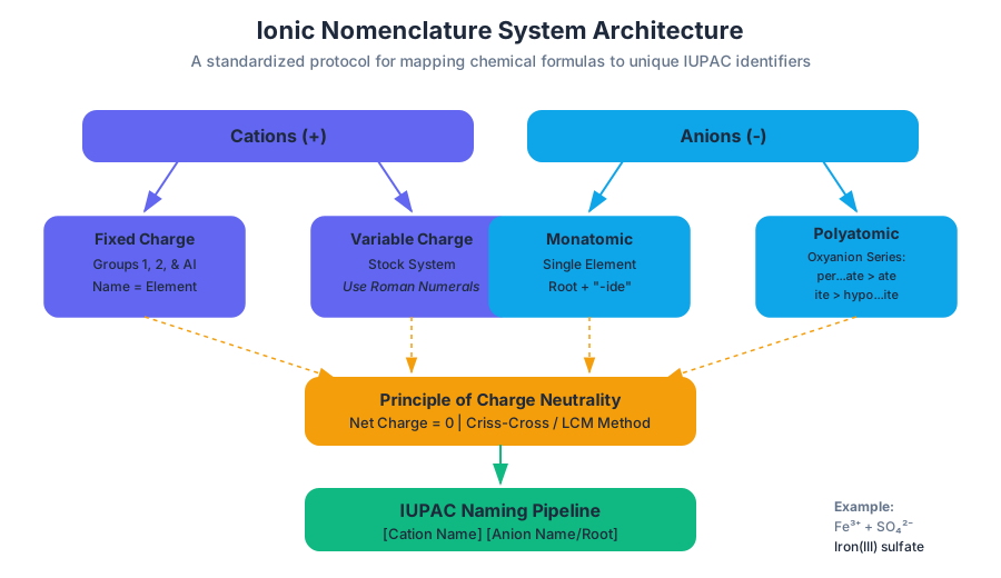
In the rigorous landscape of chemical informatics and structural chemistry, Nomenclature is more than a set of naming conventions; it is a standardized protocol for the lossless transmission of structural data. Just as a software engineer relies on a strictly defined API to ensure interoperability between systems, a chemist uses the IUPAC (International Union of Pure and Applied Chemistry) nomenclature system to ensure that the name of a compound maps uniquely and perfectly to its chemical formula and vice versa.
Ionic nomenclature specifically deals with compounds held together by electrostatic forces—the attraction between positively charged cations and negatively charged anions. This article deconstructs the logic of ionic naming, the behavior of complex polyatomic ions, and the algorithmic approach to formula construction.
The Foundation: Oxidation States and Charge Neutrality
Before naming a compound, one must understand the Oxidation State (or oxidation number). This is a theoretical value representing the number of electrons an atom loses or gains to achieve a stable, often noble-gas-like, electron configuration.
The Principle of Charge Neutrality: A stable ionic compound must have a net charge of zero. The total positive charge contributed by the cations must exactly equal the total negative charge contributed by the anions.
This principle is the "unit test" for any chemical formula. If the charges do not sum to zero, the formula is chemically non-viable under standard conditions.
Fixed vs. Variable Charges
Elements in the periodic table generally follow predictable patterns based on their valence shells. However, the transition metals (Groups 3–12) often exhibit multiple oxidation states due to the proximity of their s and d orbital energy levels.
| Group / Element | Common Ion | Charge | Classification |
|---|---|---|---|
| Group 1 (Alkali Metals) | $Li^+, Na^+, K^+$ | +1 | Fixed |
| Group 2 (Alkaline Earth) | $Mg^{2+}, Ca^{2+}, Ba^{2+}$ | +2 | Fixed |
| Group 17 (Halogens) | $F^-, Cl^-, Br^-$ | -1 | Fixed (in binary) |
| Group 16 (Chalcogens) | $O^{2-}, S^{2-}$ | -2 | Fixed (in binary) |
| Iron (Fe) | $Fe^{2+}, Fe^{3+}$ | +2, +3 | Variable |
| Copper (Cu) | $Cu^+, Cu^{2+}$ | +1, +2 | Variable |
Binary Ionic Compounds (Type I and Type II)
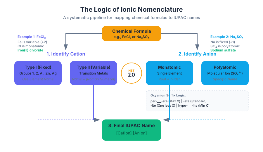
A Binary Ionic Compound consists of exactly two elements: a metal and a non-metal. The naming convention follows a simple pipeline: [Cation Name] [Anion Root + "-ide"].
Type I: Fixed Charge Cations
For metals in Groups 1, 2, and Aluminum, the charge is invariant. We do not specify the charge in the name because it is implied by the element's position on the periodic table.
- $NaCl$: Sodium chloride
- $Al_2O_3$: Aluminum oxide
Type II: Variable Charge Cations (The Stock System)
When dealing with transition metals that can form multiple ions, we use the Stock System, which employs Roman numerals in parentheses to denote the oxidation state of the metal.
- $FeCl_2$: Iron(II) chloride (Iron is +2)
- $FeCl_3$: Iron(III) chloride (Iron is +3)
Common Pitfall: A frequent error is assuming the Roman numeral refers to the subscript in the formula. It does not. It refers strictly to the charge of the individual metal ion.
Polyatomic Ions: The Molecular Ions
Polyatomic ions are covalently bonded groups of atoms that carry a net charge and behave as a single, indivisible unit during ionic bonding. They are the "objects" or "structs" of the chemical world—internally complex but treated as a single entity by the external system.
The Oxyanion Series
Most polyatomic ions are oxyanions, consisting of an element (usually a non-metal) bonded to varying numbers of oxygen atoms. These follow a systematic suffix/prefix pattern based on the oxygen count relative to the "standard" -ate form.
| Prefix | Suffix | Oxygen Level | Example (Chlorine series) | Name |
|---|---|---|---|---|
| per- | -ate | Highest | $ClO_4^-$ | Perchlorate |
| (none) | -ate | Standard | $ClO_3^-$ | Chlorate |
| (none) | -ite | One Less | $ClO_2^-$ | Chlorite |
| hypo- | -ite | Lowest | $ClO^-$ | Hypochlorite |
Common Polyatomic Ions to Memorize
In chemical practice, certain ions appear with such frequency that they must be committed to memory.
| Ion Name | Formula | Charge |
|---|---|---|
| Ammonium | $NH_4^+$ | +1 |
| Hydroxide | $OH^-$ | -1 |
| Nitrate | $NO_3^-$ | -1 |
| Sulfate | $SO_4^{2-}$ | -2 |
| Carbonate | $CO_3^{2-}$ | -2 |
| Phosphate | $PO_4^{3-}$ | -3 |
| Acetate | $C_2H_3O_2^-$ | -1 |
Algorithmic Formula Construction
Writing a formula requires balancing the charges of the cation and anion. While many students use the "Criss-Cross Method," it is more robust to view this as a Least Common Multiple (LCM) problem.
The Criss-Cross Method
- Write the symbols for the cation and anion with their charges.
- Take the magnitude of the cation's charge and make it the subscript of the anion.
- Take the magnitude of the anion's charge and make it the subscript of the cation.
- Reduce the subscripts to the lowest whole-number ratio.
Example: Aluminum Oxide
- Ions: $Al^{3+}$ and $O^{2-}$
- Criss-cross: $Al_2O_3$
- Ratio (2:3) is already irreducible. Final formula: $Al_2O_3$.
Example: Magnesium Oxide
- Ions: $Mg^{2+}$ and $O^{2-}$
- Criss-cross: $Mg_2O_2$
- Reduce: $MgO$ (Since 2:2 simplifies to 1:1).
Implementation in Code
The following Python implementation demonstrates the logic of finding the lowest whole-number ratio for an ionic compound given two oxidation states.
import math

def balance_ionic_compound(cation_symbol, cation_charge, anion_symbol, anion_charge):
    """
    Calculates the subscripts for a neutral ionic compound.
    Args:
        cation_charge (int): The positive charge of the metal.
        anion_charge (int): The negative charge of the non-metal (as a negative int).
    Returns:
        string: The chemical formula.
    """
    # Use absolute values for calculation
    c_charge = abs(cation_charge)
    a_charge = abs(anion_charge)

    # Find the Least Common Multiple
    lcm = abs(c_charge * a_charge) // math.gcd(c_charge, a_charge)

    # Calculate subscripts
    cation_subscript = lcm // c_charge
    anion_subscript = lcm // a_charge

    # Format strings (omit '1')
    c_sub = str(cation_subscript) if cation_subscript > 1 else ""
    a_sub = str(anion_subscript) if anion_subscript > 1 else ""

    return f"{cation_symbol}{c_sub}{anion_symbol}{a_sub}"

# Example: Iron(III) Sulfate
# Fe (+3), SO4 (-2)
print(balance_ionic_compound("Fe", 3, "(SO4)", -2))
# Output: Fe2(SO4)3
Mathematical Derivation of Charge Neutrality
The requirement for a neutral compound can be expressed as a linear Diophantine equation where the variables are the subscripts (integers) and the coefficients are the charges.
n_{cation} \cdot Z_{cation} + n_{anion} \cdot Z_{anion} = 0
Where:
- $n_{cation}, n_{anion} \in \mathbb{Z}^+$ (Subscripts must be positive integers)
- $Z_{cation}$ is the positive charge.
- $Z_{anion}$ is the negative charge.
To find the empirical formula (the simplest ratio), we solve for the smallest integers $n_{cation}$ and $n_{anion}$ that satisfy the equation. This is equivalent to:
\frac{n_{cation}}{n_{anion}} = \left| \frac{Z_{anion}}{Z_{cation}} \right|
The resulting fraction must be simplified by dividing both the numerator and denominator by their greatest common divisor (GCD).
Advanced Nomenclature: Hydrates
Many ionic compounds, when crystallized from aqueous solutions, trap water molecules within their crystal lattice. These are known as Hydrates.
Naming hydrates involves:
- Naming the ionic compound normally.
- Adding the word "hydrate" with a Greek prefix indicating the number of water molecules.
| Prefix | Number | Example Formula | Name |
|---|---|---|---|
| Mono- | 1 | $CuSO_4 \cdot H_2O$ | Copper(II) sulfate monohydrate |
| Di- | 2 | $BaCl_2 \cdot 2H_2O$ | Barium chloride dihydrate |
| Tri- | 3 | $FeCl_3 \cdot 3H_2O$ | Iron(III) chloride hexahydrate |
| Penta- | 5 | $CuSO_4 \cdot 5H_2O$ | Copper(II) sulfate pentahydrate |
| Hexa- | 6 | $CoCl_2 \cdot 6H_2O$ | Cobalt(II) chloride hexahydrate |
| Hepta- | 7 | $MgSO_4 \cdot 7H_2O$ | Magnesium sulfate heptahydrate |
Computational Representation and Databases
In modern chemistry, nomenclature is often handled by software. Large-scale databases like PubChem or ChemSpider store these as relational records. A simplified SQL schema for managing a chemical inventory of ionic compounds might look like this:
-- Schema for Chemical Inventory Management
CREATE TABLE Elements (
    element_id INT PRIMARY KEY,
    symbol VARCHAR(3) NOT NULL,
    name VARCHAR(50) NOT NULL,
    standard_oxidation_state INT
);

CREATE TABLE PolyatomicIons (
    ion_id INT PRIMARY KEY,
    formula VARCHAR(20) NOT NULL,
    common_name VARCHAR(50) NOT NULL,
    charge INT NOT NULL
);

CREATE TABLE IonicCompounds (
    compound_id SERIAL PRIMARY KEY,
    cation_id INT,
    anion_id INT,
    cation_type VARCHAR(10) CHECK (cation_type IN ('element', 'polyatomic')),
    anion_type VARCHAR(10) CHECK (anion_type IN ('element', 'polyatomic')),
    iupac_name VARCHAR(255),
    formula VARCHAR(100),
    molecular_weight DECIMAL(10, 4)
);

-- Query to find all compounds containing the Sulfate ion
SELECT iupac_name, formula
FROM IonicCompounds
WHERE anion_id = (SELECT ion_id FROM PolyatomicIons WHERE common_name = 'Sulfate');
Common Pitfalls and Edge Cases
1. Parentheses Usage
A common mistake is forgetting parentheses around polyatomic ions when a subscript is required.
- Incorrect: $MgOH_2$ (This implies 1 Magnesium, 1 Oxygen, and 2 Hydrogens).
- Correct: $Mg(OH)_2$ (This correctly implies 1 Magnesium and 2 Hydroxide units).
- Note: Parentheses are only used if the subscript for the polyatomic ion is 2 or greater. $NaNO_3$ does not need them.
2. The "Silver and Zinc" Exception
While most transition metals require Roman numerals, Silver ($Ag^+$), Zinc ($Zn^{2+}$), and Cadmium ($Cd^{2+}$) almost always form only one charge. In many conventions, the Roman numeral is omitted for these (e.g., "Zinc chloride" instead of "Zinc(II) chloride"), though the Stock system version is technically not "wrong."
3. Mercury(I)
Mercury(I) is a strange outlier. It exists as a diatomic cation: $Hg_2^{2+}$. This means that even though the "average" charge per mercury atom is +1, they always travel in pairs.
- Mercury(I) chloride is $Hg_2Cl_2$, not $HgCl$.
4. Naming via CLI
In a laboratory setting, one might use a command-line tool or a library like mendeleev or rdkit to parse names.
# Example of using a hypothetical chemical parser (chem-parse)
# to validate a name and return the formula

$ chem-parse --validate "Iron(III) phosphate"
> Name: Iron(III) phosphate
> Cation: Fe (Charge: +3)
> Anion: PO4 (Charge: -3)
> Result: FePO4
> Status: VALID

$ chem-parse --formula "Calcium chloride"
> CaCl2
Summary of the Naming Pipeline
- Identify the Ions: Split the compound into its cation (positive) and anion (negative) components.
- Check for Variable Charge: If the cation is a transition metal (excluding Ag, Zn, Cd), determine its charge based on the anion.
- Identify Polyatomics: Recognize groups like $SO_4$ or $NH_4$ and use their specific names.
- Assemble the Name: [Cation] + (Roman Numeral if needed) + [Anion].
- Verify Neutrality: Ensure $(Subscript \times Charge){cation} + (Subscript \times Charge){anion} = 0$.
Stoichiometry and the Mole
Key concepts: The Mole · Avogadro's Number · Molar Mass · Stoichiometric calculations
Quantitative chemistry focusing on the mole concept and calculating relationships in chemical reactions.
Stoichiometry and the Mole
Stoichiometry is the quantitative engine of chemistry. Derived from the Greek words stoicheion (element) and metron (measure), it represents the mathematical framework used to relate the quantities of reactants and products in chemical reactions. At its core, stoichiometry is a system of chemical accounting that ensures the Law of Conservation of Mass is satisfied across every transformation of matter.
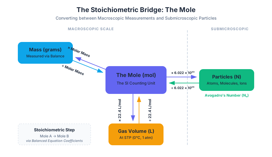
To master stoichiometry, one must navigate the transition between the submicroscopic scale—where individual atoms and molecules interact—and the macroscopic scale, where we measure substances in grams and liters. The bridge between these two worlds is the Mole.
The Mole: The Macroscopic Bridge
The fundamental challenge in chemistry is that atoms are too small to count individually. A single drop of water contains approximately $1.67 \times 10^{21}$ molecules. To handle such vast numbers, chemists use a counting unit called the Mole (abbreviated as mol).
Definition: The Mole A mole is defined as the amount of substance that contains exactly $6.02214076 \times 10^{23}$ elementary entities (atoms, molecules, ions, or electrons). This fixed numerical value is known as Avogadro’s Number ($N_A$).
Avogadro’s Number ($N_A$)
The value of $N_A$ was historically linked to the number of atoms in 12 grams of pure Carbon-12. However, as of the 2019 redefinition of the SI base units, the mole is defined by fixing the numerical value of the Avogadro constant.
| Concept | Value / Unit | Description |
|---|---|---|
| Avogadro's Number ($N_A$) | $6.022 \times 10^{23} \text{ mol}^{-1}$ | The number of particles in one mole. |
| Molar Volume (STP) | $22.414 \text{ L/mol}$ | Volume of 1 mole of ideal gas at 0°C and 1 atm. |
| Atomic Mass Unit (amu) | $1.6605 \times 10^{-24} \text{ g}$ | $1/12$ the mass of a single Carbon-12 atom. |
| The Mole (mol) | SI Base Unit | Represents a specific quantity of matter. |
Why the Mole Matters
Without the mole, chemical equations would remain qualitative "recipes" rather than quantitative instructions. The mole allows us to:
- Count by weighing: By knowing the mass of a sample, we can calculate the exact number of atoms present.
- Maintain proportionality: Chemical reactions occur in discrete ratios (e.g., 2 H₂ + 1 O₂ → 2 H₂O). The mole allows us to scale these ratios up to measurable laboratory quantities.
Molar Mass and Isotopic Abundance
While the mole tells us how many particles we have, Molar Mass ($M$) tells us the mass of those particles. Molar mass is expressed in grams per mole (g/mol).
Calculating Average Atomic Mass
The mass listed for an element on the periodic table is not the mass of a single atom, but a weighted average of all naturally occurring isotopes.
$$A_{avg} = \sum (f_i \times m_i)$$
Where $f_i$ is the fractional abundance of isotope $i$, and $m_i$ is the mass of that isotope.
From Formula to Molar Mass
To find the molar mass of a compound, we sum the atomic masses of all constituent atoms.
Example: Molar Mass of Calcium Nitrate $Ca(NO_3)_2$
- $Ca$: $1 \times 40.08 \text{ g/mol} = 40.08$
- $N$: $2 \times 14.01 \text{ g/mol} = 28.02$
- $O$: $6 \times 16.00 \text{ g/mol} = 96.00$
- Total: $164.10 \text{ g/mol}$
The following Python script demonstrates a non-trivial parser for calculating molar masses from chemical formulas, handling nested parentheses and element counts.
import re

def get_molar_mass(formula):
    """
    Calculates the molar mass of a chemical formula.
    Supports nested parentheses, e.g., Mg(HCO3)2.
    """
    periodic_table = {
        "H": 1.008, "He": 4.0026, "Li": 6.94, "Be": 9.0122, "B": 10.81,
        "C": 12.011, "N": 14.007, "O": 15.999, "F": 18.998, "Mg": 24.305,
        "Al": 26.982, "S": 32.06, "Cl": 35.45, "Ca": 40.078, "Fe": 55.845
    }

    def parse_formula(f):
        stack = [{}]
        i = 0
        while i < len(f):
            if f[i] == '(':
                stack.append({})
                i += 1
            elif f[i] == ')':
                i += 1
                start = i
                while i < len(f) and f[i].isdigit():
                    i += 1
                multiplier = int(f[start:i] or 1)
                popped = stack.pop()
                for el, count in popped.items():
                    stack[-1][el] = stack[-1].get(el, 0) + count * multiplier
            else:
                match = re.match(r'([A-Z][a-z]*)(\d*)', f[i:])
                if match:
                    el, count = match.groups()
                    count = int(count or 1)
                    stack[-1][el] = stack[-1].get(el, 0) + count
                    i += len(match.group())
                else:
                    i += 1
        return stack[0]

    counts = parse_formula(formula)
    total_mass = sum(periodic_table.get(el, 0) * count for el, count in counts.items())
    return round(total_mass, 3)

# Example Usage
compounds = ["Ca(NO3)2", "Mg(HCO3)2", "H2O", "Fe2(SO4)3"]
for c in compounds:
    print(f"Molar Mass of {c}: {get_molar_mass(c)} g/mol")
The Stoichiometric Pipeline: Mole-to-Mole Ratios
The heart of stoichiometry is the balanced chemical equation. The coefficients in a balanced equation represent the molar ratios between reactants and products.
The Law of Conservation of Mass
In a closed system, mass is neither created nor destroyed. Therefore, the number of atoms of each element must be identical on both the reactant and product sides of the equation.
The Mathematical Derivation of the Conversion Factor
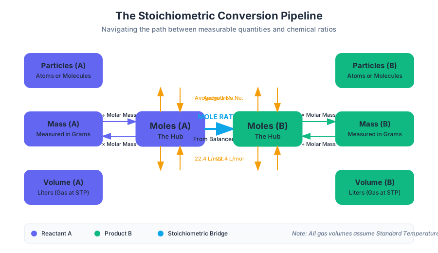
To convert from a known quantity of substance A to an unknown quantity of substance B, we utilize the stoichiometric ratio derived from the balanced equation.
\text{Quantity B} = \text{Mass A (g)} \times \frac{1 \text{ mol A}}{\text{Molar Mass A (g)}} \times \frac{\text{moles B (coeff)}}{\text{moles A (coeff)}} \times \frac{\text{Molar Mass B (g)}}{1 \text{ mol B}}
This "dimensional analysis" ensures that all units cancel out except for the desired unit of the target substance.
| Step | Operation | Unit Transformation |
|---|---|---|
| 1 | Divide by Molar Mass of A | Grams A $\rightarrow$ Moles A |
| 2 | Multiply by Mole Ratio (B/A) | Moles A $\rightarrow$ Moles B |
| 3 | Multiply by Molar Mass of B | Moles B $\rightarrow$ Grams B |
| 4 | (Optional) Density/Molarity | Grams $\rightarrow$ Volume |
Limiting Reactants and Percent Yield
In real-world applications, reactants are rarely present in exact stoichiometric proportions. One reactant will inevitably be exhausted first, halting the reaction. This is the Limiting Reactant.
Identifying the Limiting Reactant
To identify the limiting reactant, calculate the amount of product that could be formed from each reactant independently. The reactant that produces the least amount of product is the limiting reactant.
Percent Yield
The Theoretical Yield is the maximum amount of product calculated via stoichiometry. The Actual Yield is the amount physically collected in the lab.
$$\text{Percent Yield} = \left( \frac{\text{Actual Yield}}{\text{Theoretical Yield}} \right) \times 100%$$
Insight: Why isn't yield 100%? Low yields often result from side reactions, incomplete reactions, loss of product during filtration/transfer, or the existence of chemical equilibrium.
The following shell script demonstrates how a researcher might use a CLI tool to calculate yield and log it to a database.
#!/bin/bash

# Chemical Yield Calculator CLI
# Usage: ./yield_calc.sh [actual_mass] [theoretical_mass] [experiment_id]

ACTUAL=$1
THEORETICAL=$2
EXP_ID=$3

if [[ -z "$ACTUAL" || -z "$THEORETICAL" ]]; then
    echo "Error: Missing parameters."
    echo "Usage: ./yield_calc.sh [actual] [theoretical] [id]"
    exit 1
fi

# Calculate percent yield using 'bc' for floating point math
PERCENT_YIELD=$(echo "scale=2; ($ACTUAL / $THEORETICAL) * 100" | bc)

echo "--- Experiment $EXP_ID Report ---"
echo "Theoretical Yield: $THEORETICAL g"
echo "Actual Yield:      $ACTUAL g"
echo "Percent Yield:     $PERCENT_YIELD%"

# Log to a simulated database file
echo "$(date '+%Y-%m-%d %H:%M:%S'),$EXP_ID,$ACTUAL,$THEORETICAL,$PERCENT_YIELD" >> experiment_log.csv
Advanced Stoichiometry: Solutions and Gases
Stoichiometry extends beyond solids into the realms of liquids (solutions) and gases.
Solution Stoichiometry (Molarity)
Concentration is typically expressed as Molarity ($M$), which is moles of solute per liter of solution.
$$M = \frac{n \text{ (mol)}}{V \text{ (L)}}$$
When performing stoichiometry with solutions, the volume and molarity are used to find the number of moles: $n = M \times V$.
Gas Stoichiometry
For reactions involving gases, the Ideal Gas Law ($PV = nRT$) allows for the conversion between gas volume and moles. At Standard Temperature and Pressure (STP: 0°C, 1 atm), 1 mole of any ideal gas occupies 22.4 liters.
| Parameter | Symbol | Units |
|---|---|---|
| Pressure | $P$ | atm, kPa, mmHg |
| Volume | $V$ | Liters (L) |
| Moles | $n$ | mol |
| Gas Constant | $R$ | $0.0821 \text{ L}\cdot\text{atm/mol}\cdot\text{K}$ |
| Temperature | $T$ | Kelvin (K) |
Common Pitfalls in Stoichiometric Calculations
Even experienced chemists can make errors in complex stoichiometric pipelines. Understanding these common failure points is essential for accuracy.
| Pitfall | Description | Correction |
|---|---|---|
| Using Mass Ratios | Attempting to use the mass of reactants directly in the ratio (e.g., 2g H₂ reacts with 1g O₂). | Always convert mass to moles before using the stoichiometric ratio. |
| Unbalanced Equations | Forgetting to balance the equation before starting calculations. | Check that the number of atoms on both sides is equal. |
| Incorrect Molar Mass | Forgetting to account for subscripts (e.g., using 16.00 for $O_2$ instead of 32.00). | Double-check the molecular formula and atomic weights. |
| Sig Fig Errors | Losing precision by rounding too early in a multi-step calculation. | Keep all digits in the calculator until the final step. |
| STP Assumptions | Assuming $22.4 \text{ L/mol}$ when the reaction is not at 0°C or 1 atm. | Use $PV=nRT$ for non-standard conditions. |
Worked Example: The Combustion of Octane
Consider the combustion of octane ($C_8H_{18}$) in an engine:
2 C_8H_{18} + 25 O_2 \rightarrow 16 CO_2 + 18 H_2O
If we burn 100g of octane, how many grams of $CO_2$ are produced?
- Molar Mass of Octane: $(8 \times 12.01) + (18 \times 1.008) = 114.23 \text{ g/mol}$
- Moles of Octane: $100 \text{ g} / 114.23 \text{ g/mol} = 0.8754 \text{ mol}$
- Mole Ratio: $16 \text{ mol } CO_2 / 2 \text{ mol } C_8H_{18} = 8$
- Moles of $CO_2$: $0.8754 \text{ mol} \times 8 = 7.0032 \text{ mol}$
- Molar Mass of $CO_2$: $12.01 + (2 \times 16.00) = 44.01 \text{ g/mol}$
- Mass of $CO_2$: $7.0032 \text{ mol} \times 44.01 \text{ g/mol} = 308.21 \text{ g}$
This calculation shows that burning 100g of fuel results in over 300g of $CO_2$ gas, a non-intuitive result that highlights the importance of accounting for the oxygen consumed from the atmosphere.
States of Matter and Intermolecular Forces
Key concepts: Kinetic Molecular Theory · Intermolecular Forces (IMF) · Phase Changes · Hydrogen Bonding
Analysis of solids, liquids, and gases, and the forces that act between molecules.
States of Matter and Intermolecular Forces
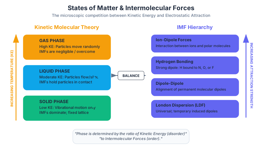
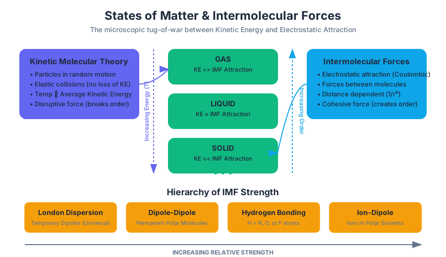
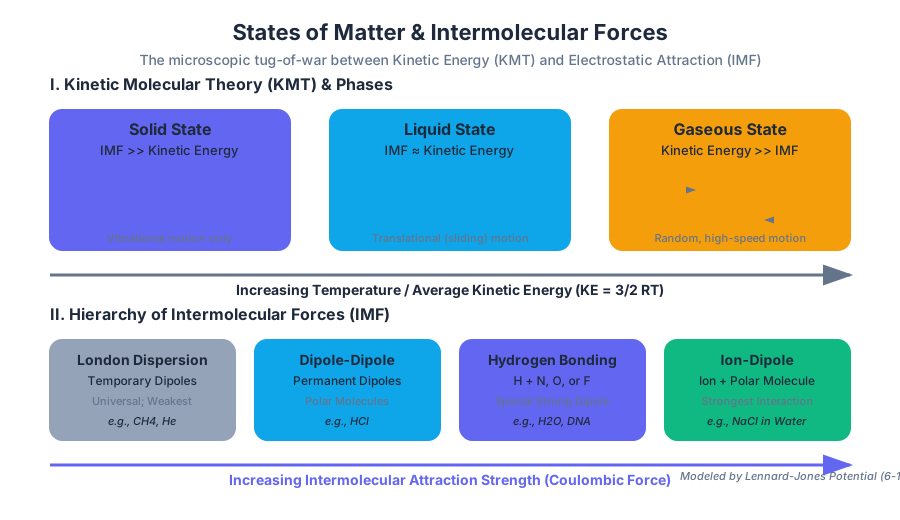
The macroscopic world we perceive—the rigidity of a diamond, the fluidity of a river, the invisibility of the air—is a direct consequence of a silent tug-of-war occurring at the nanometer scale. While chemical bonding (intramolecular forces) dictates the identity of a molecule, Intermolecular Forces (IMF) dictate its behavior in bulk. This section explores the Kinetic Molecular Theory (KMT) as the framework for understanding particle motion and the specific electrostatic interactions that determine the phase and physical properties of matter.
Kinetic Molecular Theory (KMT)
What it is
The Kinetic Molecular Theory (KMT) is a conceptual model used to explain the behavior of matter, particularly gases, by treating individual particles as point masses in constant, random motion. While originally developed for "Ideal Gases," its principles extend to liquids and solids by accounting for the decreasing mean free path between particles.
Why it matters
KMT provides the theoretical bridge between microscopic particle behavior (velocity, collisions) and macroscopic observables (temperature, pressure, volume). It allows us to derive the Ideal Gas Law ($PV = nRT$) and understand why substances change phase when energy is added or removed.
How it works: The Five Postulates
- Negligible Volume: The particles are so small compared to the distances between them that their individual volume is assumed to be zero.
- Random Motion: Particles move in straight lines in all directions until they collide.
- No Intermolecular Forces: In an ideal gas, particles do not attract or repel each other. (Note: This is the primary point where real matter diverges from KMT).
- Elastic Collisions: Kinetic energy is transferred between particles during collisions, but the total kinetic energy of the system remains constant.
- Temperature as Kinetic Energy: The average kinetic energy ($KE_{avg}$) of a gas is directly proportional to its absolute temperature (Kelvin).
The Fundamental Equation of KMT: $$KE_{avg} = \frac{3}{2}RT = \frac{1}{2}mv_{rms}^2$$ Where $R$ is the gas constant, $T$ is temperature, $m$ is mass, and $v_{rms}$ is the root-mean-square velocity.
Concrete Example: Particle Simulation
To visualize KMT, we can implement a basic particle engine. In this low-level C implementation, we simulate particles in a 2D box, demonstrating how velocity and collisions (though simplified) result in pressure against the container walls.
#include <stdio.h>

typedef struct {
    double x, y;   // Position
    double vx, vy; // Velocity
    double mass;
} Particle;

// Update particle position based on KMT postulates (straight-line motion)
void update_position(Particle *p, double dt, double box_width, double box_height) {
    p->x += p->vx * dt;
    p->y += p->vy * dt;

    // Elastic collision with walls: velocity is reversed, energy is conserved
    if (p->x <= 0 || p->x >= box_width) {
        p->vx *= -1;
        // Force exerted on the wall here contributes to macroscopic Pressure
    }
    if (p->y <= 0 || p->y >= box_height) {
        p->vy *= -1;
    }
}

int main() {
    Particle gas_particle = {5.0, 5.0, 150.0, 120.0, 1.0};
    double delta_t = 0.01;

    for(int i = 0; i < 100; i++) {
        update_position(&gas_particle, delta_t, 100.0, 100.0);
        printf("Step %d: Position(%.2f, %.2f)\n", i, gas_particle.x, gas_particle.y);
    }
    return 0;
}
Common Pitfalls
A common misconception is that all particles in a sample move at the same speed. In reality, they follow the Maxwell-Boltzmann Distribution, a probability distribution where temperature shifts the peak (most probable speed) and spreads the curve.
Intermolecular Forces (IMF)
What it is
Intermolecular Forces are the attractive forces that exist between molecules. They are significantly weaker than intramolecular bonds (ionic or covalent) but are responsible for the existence of condensed phases (liquids and solids).
Why it matters
Without IMFs, the entire universe would be a gas. IMFs determine boiling points, melting points, viscosity, surface tension, and vapor pressure. In engineering, understanding IMFs is critical for material selection, lubricant design, and pharmaceutical drug delivery.
How it works: The Hierarchy of Strength
IMFs are essentially electrostatic in nature, governed by Coulomb's Law ($F = k \frac{q_1 q_2}{r^2}$). The strength depends on the magnitude of the charges and the distance between them.
| Force Type | Source | Relative Strength | Example |
|---|---|---|---|
| London Dispersion (LDF) | Induced/Temporary Dipoles | Weakest (but universal) | $CH_4$, $He$, $N_2$ |
| Dipole-Dipole | Permanent Dipoles | Moderate | $HCl$, $CH_3Cl$ |
| Hydrogen Bonding | H bound to N, O, or F | Strong | $H_2O$, $NH_3$, DNA |
| Ion-Dipole | Ion + Polar Molecule | Very Strong | $NaCl(aq)$ |
The Lennard-Jones Potential
The interaction between two non-bonded particles is often modeled using the Lennard-Jones 6-12 Potential. This mathematical representation accounts for both the attractive forces (Van der Waals) and the Pauli repulsion at very short distances.
V_{LJ}(r) = 4\epsilon \left[ \left( \frac{\sigma}{r} \right)^{12} - \left( \frac{\sigma}{r} \right)^{6} \right]
Where:
- $V$ is the intermolecular potential between the two particles.
- $\epsilon$ is the depth of the potential well (strength of attraction).
- $\sigma$ is the distance at which the potential is zero (particle size).
- $r$ is the distance between particles.
- The $r^{-12}$ term represents repulsion (electron cloud overlap).
- The $r^{-6}$ term represents attraction (dispersion forces).
Deep Dive: Hydrogen Bonding
What it is
Hydrogen Bonding is a specific, unusually strong type of dipole-dipole interaction. It occurs when a hydrogen atom is covalently bonded to a highly electronegative atom (N, O, or F), creating a significant partial positive charge on the hydrogen.
Why it matters
Hydrogen bonding is the reason water expands when it freezes (creating the open hexagonal lattice of ice), why DNA strands stay together but can be "unzipped," and why proteins fold into specific 3D shapes.
How it works: The "Perfect Storm" of Factors
- High Electronegativity: N, O, and F pull electron density away from H, leaving it nearly a "naked proton."
- Small Atomic Radius: Because H is small and the lone pairs on N, O, or F are concentrated in a small volume, the molecules can get very close to each other, maximizing the Coulombic attraction ($r$ is small in $1/r^2$).
Concrete Example: Boiling Point Anomalies
If we look at the boiling points of Group 16 hydrides ($H_2S, H_2Se, H_2Te$), we see a steady increase due to increasing LDFs. However, $H_2O$ is a massive outlier with a boiling point of 100°C, whereas $H_2S$ is -60°C. This "jump" is the signature of hydrogen bonding.
Phase Changes and Thermodynamics
What it is
A Phase Change is a physical transformation of a substance from one state of matter to another. These changes are nearly always isothermal (occurring at a constant temperature) as the energy added is used to overcome IMFs rather than increasing particle velocity.
How it works: Energy Calculations
To calculate the energy required to change the phase of a substance, we use the Enthalpy of Fusion ($\Delta H_{fus}$) for melting and the Enthalpy of Vaporization ($\Delta H_{vap}$) for boiling.
| Phase Change | Direction | Energy Change | Terminology |
|---|---|---|---|
| Solid $\rightarrow$ Liquid | Endothermic | $+\Delta H_{fus}$ | Melting / Fusion |
| Liquid $\rightarrow$ Solid | Exothermic | $-\Delta H_{fus}$ | Freezing / Crystallization |
| Liquid $\rightarrow$ Gas | Endothermic | $+\Delta H_{vap}$ | Boiling / Vaporization |
| Gas $\rightarrow$ Liquid | Exothermic | $-\Delta H_{vap}$ | Condensation |
| Solid $\rightarrow$ Gas | Endothermic | $+\Delta H_{sub}$ | Sublimation |
Worked Example: The Energy of Steam
How much energy is required to convert 50g of ice at -10°C to steam at 110°C? This requires a multi-step calculation using specific heat capacities ($c$) and enthalpies.
import numpy as np

def calculate_total_energy(mass, temp_initial, temp_final):
    # Constants for Water
    c_ice = 2.09      # J/g°C
    c_liquid = 4.18   # J/g°C
    c_steam = 2.01    # J/g°C
    H_fus = 334       # J/g
    H_vap = 2260      # J/g

    energy = 0

    # 1. Heat ice to 0°C
    if temp_initial < 0:
        energy += mass * c_ice * (0 - temp_initial)
        print(f"Heating ice: {energy:.2f} J")

    # 2. Melt ice at 0°C
    energy += mass * H_fus
    print(f"Melting ice: {mass * H_fus:.2f} J")

    # 3. Heat water to 100°C
    energy += mass * c_liquid * (100 - 0)
    print(f"Heating water: {mass * c_liquid * 100:.2f} J")

    # 4. Vaporize water at 100°C
    energy += mass * H_vap
    print(f"Vaporizing water: {mass * H_vap:.2f} J")

    # 5. Heat steam to final temp
    if temp_final > 100:
        energy += mass * c_steam * (temp_final - 100)
        print(f"Heating steam: {mass * c_steam * (temp_final - 100):.2f} J")

    return energy

total_j = calculate_total_energy(50, -10, 110)
print(f"\nTotal Energy Required: {total_j / 1000:.2f} kJ")
Phase Diagrams and the Critical Point
What it is
A Phase Diagram is a graphical representation of the physical states of a substance under different conditions of temperature and pressure.
Key Features
- Triple Point: The unique temperature and pressure where all three phases (solid, liquid, gas) coexist in equilibrium.
- Critical Point: The temperature and pressure beyond which the distinction between liquid and gas disappears, resulting in a Supercritical Fluid.
- The Phase Boundary Lines: Lines representing equilibrium between two phases (e.g., the boiling point curve).
Variations: The Water Anomaly
Most substances have a solid-liquid equilibrium line with a positive slope (increasing pressure favors the denser solid phase). Water is a rare exception; its line has a negative slope. Increasing pressure on ice can actually cause it to melt into liquid water because liquid water is denser than ice (due to the collapse of the hydrogen-bonded lattice).
Vapor Pressure and Volatility
What it is
Vapor Pressure is the pressure exerted by a vapor in thermodynamic equilibrium with its condensed phase (solid or liquid) at a given temperature in a closed system.
How it works: The Clausius-Clapeyron Equation
The relationship between vapor pressure and temperature is non-linear. As temperature increases, the fraction of molecules with enough kinetic energy to escape the IMFs of the liquid increases exponentially.
Clausius-Clapeyron Equation: $$\ln(P) = -\frac{\Delta H_{vap}}{R} \left( \frac{1}{T} \right) + C$$ This shows that a plot of $\ln(P)$ vs $1/T$ yields a straight line with a slope related to the heat of vaporization.
Real-World Usage: Atmospheric Pressure and Cooking
Boiling occurs when Vapor Pressure = Atmospheric Pressure.
- At sea level (1 atm), water boils at 100°C.
- At high altitudes (lower atmospheric pressure), water's vapor pressure reaches the atmospheric threshold at a lower temperature (e.g., 95°C in Denver). This is why "high-altitude cooking" instructions require longer boiling times—the water simply isn't as hot.
# Example: Using a hypothetical CLI tool 'chemprop' to find boiling points
# at different pressures (simulated output)

$ chemprop boiling-point H2O --pressure 0.83atm
> Substance: Water (H2O)
> Pressure: 0.83 atm (approx. 5000ft altitude)
> Calculated Boiling Point: 94.62°C
> IMF Profile: Strong Hydrogen Bonding, High Delta-H-Vap
Summary of Physical Property Trends
The strength of IMFs dictates almost every physical property of a liquid.
| Property | Definition | Relationship to IMF Strength |
|---|---|---|
| Boiling Point | Temp where vapor pressure = external pressure | Direct (Stronger IMF = Higher BP) |
| Vapor Pressure | Pressure of gas above its liquid | Inverse (Stronger IMF = Lower VP) |
| Viscosity | Resistance to flow | Direct (Stronger IMF = More "sticky") |
| Surface Tension | Energy required to increase surface area | Direct (Stronger IMF = Higher Tension) |
| Volatility | Ease of evaporation | Inverse (Stronger IMF = Less Volatile) |
Chemical Reactions and Predicting Products
Key concepts: Synthesis and Decomposition · Single and Double Replacement · Combustion · Law of Conservation of Mass
Identifying types of chemical reactions and predicting the outcomes of mixing different substances.
Chemical Reactions and Predicting Products
Chemical reactions represent the fundamental mechanism by which the universe rearranges matter. At the macroscopic level, we observe color changes, heat evolution, and the formation of new phases; at the microscopic level, reactions are the orchestrated breaking and reforming of chemical bonds, driven by the pursuit of lower Gibbs free energy. To master chemistry is to move beyond observing these changes to predicting them with mathematical and structural precision.
The Fundamental Axiom: The Law of Conservation of Mass
Before one can predict the product of a reaction, one must respect the physical constraints of the universe. The Law of Conservation of Mass, formalized by Antoine Lavoisier in 1789, states that mass is neither created nor destroyed in a chemical reaction.
The Law of Conservation of Mass: In a closed system, the mass of the reactants must exactly equal the mass of the products. Consequently, the number of atoms of each element must remain constant throughout the transformation.
This law necessitates the balancing of equations. A chemical equation is not merely a description; it is a balanced stoichiometric account. If we react hydrogen gas with oxygen gas to form water, the raw observation ($H_2 + O_2 \rightarrow H_2O$) violates this law. The balanced form ($2H_2 + O_2 \rightarrow 2H_2O$) satisfies it by ensuring four hydrogen atoms and two oxygen atoms exist on both sides of the arrow.
Mathematical Representation of Mass Balance
For any reaction $\sum \nu_i R_i \rightarrow \sum \nu_j P_j$, where $\nu$ represents the stoichiometric coefficient: $$\sum (m_{reactants}) = \sum (m_{products})$$
| Feature | Reactants | Products |
|---|---|---|
| Definition | Substances consumed during the reaction. | Substances produced by the reaction. |
| Placement | Left side of the yield arrow ($\rightarrow$). | Right side of the yield arrow ($\rightarrow$). |
| Mass Relationship | Total initial mass. | Total final mass (identical to initial). |
| Bonding State | Bonds are broken (requires energy). | Bonds are formed (releases energy). |
Synthesis and Decomposition: The Binary Logic of Matter
The simplest forms of chemical change involve the combination of multiple species into one, or the breakdown of one species into many.
Synthesis (Combination) Reactions
In a Synthesis reaction, two or more simple substances combine to form a more complex product. The general form is $A + B \rightarrow AB$. These reactions are typically exothermic, as the formation of new bonds releases more energy than is required to initiate the process.
- Metal + Nonmetal: Usually results in an ionic compound (e.g., $2Na + Cl_2 \rightarrow 2NaCl$).
- Nonmetal + Nonmetal: Results in a covalent compound (e.g., $S + O_2 \rightarrow SO_2$).
- Oxide + Water: Metal oxides form bases ($CaO + H_2O \rightarrow Ca(OH)_2$), while nonmetal oxides form acids ($SO_3 + H_2O \rightarrow H_2SO_4$).
Decomposition Reactions
Decomposition is the inverse of synthesis: $AB \rightarrow A + B$. Because these reactions involve breaking stable bonds, they almost always require an input of energy in the form of heat (pyrolysis), light (photolysis), or electricity (electrolysis).
- Carbonates: Decompose into metal oxides and carbon dioxide ($CaCO_3 \rightarrow CaO + CO_2$).
- Chlorates: Decompose into metal chlorides and oxygen gas ($2KClO_3 \rightarrow 2KCl + 3O_2$).
- Hydroxides: Decompose into metal oxides and water ($Mg(OH)_2 \rightarrow MgO + H_2O$).
Single Replacement: The Competition for Electrons
A Single Replacement (or displacement) reaction occurs when a more reactive element displaces a less reactive element from a compound: $A + BC \rightarrow AC + B$. These reactions are fundamentally Redox (Reduction-Oxidation) processes involving the transfer of electrons.
The Activity Series
To predict whether a single replacement reaction will occur, chemists utilize the Activity Series. An element can only replace an element listed below it on the series.
| Element Type | Reactivity Level | Examples | Behavior |
|---|---|---|---|
| Active Metals | High | $Li, K, Ca, Na$ | React with cold water to displace $H_2$. |
| Moderate Metals | Medium | $Mg, Al, Zn, Fe$ | React with steam or acids to displace $H_2$. |
| Noble Metals | Low | $Cu, Ag, Au, Pt$ | Do not react with water or most acids. |
| Halogens | Variable | $F > Cl > Br > I$ | Higher halogens displace lower ones. |
Worked Example: If a strip of Zinc ($Zn$) is placed in a solution of Copper(II) Sulfate ($CuSO_4$), will a reaction occur?
- Consult the Activity Series: $Zn$ is more active than $Cu$.
- Prediction: $Zn$ will displace $Cu$.
- Equation: $Zn(s) + CuSO_4(aq) \rightarrow ZnSO_4(aq) + Cu(s)$.
- Observation: The blue color of the solution fades as $Zn^{2+}$ ions form, and reddish-brown copper metal precipitates.
Double Replacement: The Metathesis Exchange
In Double Replacement reactions, the cations and anions of two different ionic compounds switch places: $AB + CD \rightarrow AD + CB$. These reactions typically occur in aqueous solutions.
Driving Forces
A double replacement reaction only occurs if one of the products is "removed" from the ion-exchange equilibrium. This happens through three primary driving forces:
- Precipitation: Formation of an insoluble solid.
- Gas Evolution: Formation of a gas (like $CO_2$ or $H_2S$).
- Molecular Formation: Formation of a stable molecular compound, most commonly water ($H_2O$) in an acid-base neutralization.
Solubility Rules
To predict the formation of a precipitate, one must apply the solubility rules:
| Soluble Compounds | Exceptions |
|---|---|
| Group 1 cations ($Li^+, Na^+$, etc.) | None |
| Ammonium ($NH_4^+$) | None |
| Nitrates ($NO_3^-$) and Acetates | None |
| Halides ($Cl^-, Br^-, I^-$) | $Ag^+, Pb^{2+}, Hg_2^{2+}$ |
| Sulfates ($SO_4^{2-}$) | $Ba^{2+}, Sr^{2+}, Pb^{2+}, Ca^{2+}$ |
Insoluble Compounds: Most Carbonates ($CO_3^{2-}$), Phosphates ($PO_4^{3-}$), and Hydroxides ($OH^-$) are insoluble unless paired with Group 1 metals or Ammonium.
Combustion: The Chemistry of Fire
Combustion is a rapid reaction between a fuel (usually a hydrocarbon) and an oxidant (oxygen gas) that produces heat and light.
Hydrocarbon Combustion
For any hydrocarbon of the form $C_xH_y$, the products of complete combustion are always carbon dioxide ($CO_2$) and water vapor ($H_2O$).
C_xH_y + (x + \frac{y}{4})O_2 \rightarrow xCO_2 + \frac{y}{2}H_2O
If oxygen is limited, incomplete combustion occurs, producing Carbon Monoxide ($CO$) or elemental Carbon (soot, $C$).
Combustion of Metals
Many metals also undergo combustion, which technically doubles as a synthesis reaction. For example, the combustion of magnesium:
2Mg(s) + O_2(g) \rightarrow 2MgO(s) + \text{light}
Algorithmic Prediction and Balancing
Predicting products requires a systematic pipeline:
- Identify Reactant Types: Are they elements or compounds?
- Classify Reaction: Use the structures ($A+B$, $AB$, $A+BC$, $AB+CD$, or $C_xH_y+O_2$).
- Determine Products: Use valency (charge balance) to write correct formulas.
- Check Feasibility: Use the Activity Series for single replacement or Solubility Rules for double replacement.
- Balance: Apply the Law of Conservation of Mass.
Implementation: Balancing via Linear Algebra
While many balance equations by inspection, complex redox reactions are best solved using a system of linear equations where each element represents a constraint.
import numpy as np
from fractions import Fraction

def balance_equation(reactants, products):
    """
    Solves for stoichiometric coefficients using a null space approach.
    Example input:
    reactants = [{'C': 3, 'H': 8}, {'O': 2}] (Propane + Oxygen)
    products = [{'C': 1, 'O': 2}, {'H': 2, 'O': 1}] (CO2 + H2O)
    """
    elements = sorted(list(set().union(*reactants, *products)))
    element_map = {el: i for i, el in enumerate(elements)}

    matrix = np.zeros((len(elements), len(reactants) + len(products)))

    for j, comp in enumerate(reactants):
        for el, count in comp.items():
            matrix[element_map[el], j] = count

    for j, comp in enumerate(products):
        for el, count in comp.items():
            matrix[element_map[el], j + len(reactants)] = -count

    # Solve for the null space (Ax = 0)
    # Using SVD for numerical stability
    u, s, vh = np.linalg.svd(matrix)
    null_space = vh[-1, :]

    # Normalize to integers
    coeffs = [abs(x) for x in null_space]
    min_val = min(coeffs)
    normalized = [round(x / min_val) for x in coeffs]

    return normalized

# Example: C3H8 + O2 -> CO2 + H2O
# Results: [1, 5, 3, 4]
Theoretical Derivation: The Driving Force of Replacement
The spontaneity of a single replacement reaction can be derived from the standard reduction potentials ($E^\circ$). A reaction is spontaneous if the cell potential ($E^\circ_{cell}$) is positive.
E^\circ_{cell} = E^\circ_{cathode} - E^\circ_{anode}

For Zn + Cu^2+ -> Zn^2+ + Cu:
E^\circ(Cu^2+/Cu) = +0.34V
E^\circ(Zn^2+/Zn) = -0.76V
E^\circ_{cell} = 0.34 - (-0.76) = +1.10V (Spontaneous)
Real-World Application: Industrial Synthesis
In industrial chemical engineering, predicting products is the first step in process design. The Haber-Bosch process is a classic synthesis reaction where the yield is maximized by manipulating equilibrium.
# Example: Using a hypothetical CLI tool 'chem-sim' to model
# the synthesis of Ammonia under specific conditions.

chem-sim predict --reactants "N2(g), H2(g)" \
                 --temp 450C \
                 --pressure 200atm \
                 --catalyst "Fe" \
                 --output-format json
Common Pitfalls in Prediction
- Ignoring Diatomic Elements: Students often write $H$ or $O$ instead of $H_2$ or $O_2$. Remember BrINClHOF (Bromine, Iodine, Nitrogen, Chlorine, Hydrogen, Oxygen, Fluorine).
- Incorrect Formulas: Predicting $NaCl_2$ because the reactant was $MgCl_2$. You must balance the charges of the new compound based on the oxidation states of the constituent ions.
- Forcing Reactions: Assuming a reaction occurs just because reactants are mixed. Always check the Activity Series and Solubility Rules.
- Balancing Subscripts: Never change the subscripts of a correctly written formula to balance an equation. Only change the coefficients.
Summary Table: Reaction Archetypes
| Reaction Type | Reactants | Products | Key Identifier |
|---|---|---|---|
| Synthesis | Two elements or simple compounds | One complex compound | $A + B \rightarrow AB$ |
| Decomposition | One complex compound | Two or more simpler substances | $AB \rightarrow A + B$ |
| Single Replacement | One element + one compound | One element + one compound | $A + BC \rightarrow AC + B$ |
| Double Replacement | Two ionic compounds | Two ionic compounds | $AB + CD \rightarrow AD + CB$ |
| Combustion | Hydrocarbon + Oxygen | $CO_2 + H_2O$ | Presence of $O_2$ and heat |
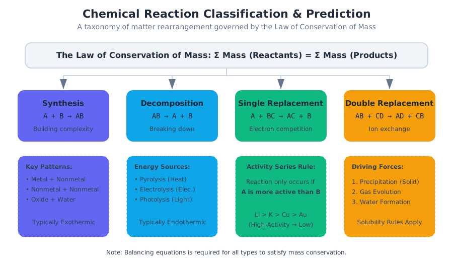
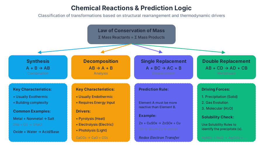
Thermodynamics and Energy
Key concepts: Enthalpy · Endothermic vs. Exothermic · Specific Heat · Hess's Law
The study of heat, work, and energy changes in chemical systems.
Thermodynamics and Energy
In the study of chemical systems, energy is the fundamental currency. Thermodynamics is the rigorous framework we use to track the exchange, transformation, and conservation of this currency. While the first law of thermodynamics dictates that energy cannot be created or destroyed, it says nothing about the form that energy takes or the ease with which it moves. To understand chemical reactions, we must look beyond simple energy conservation and into the specific behavior of heat, work, and the internal state of matter.
Enthalpy: The Heat of the System
At the heart of chemical thermodynamics is Enthalpy ($H$). While internal energy ($U$) represents the sum of all microscopic kinetic and potential energies within a system, enthalpy is a specialized "bookkeeping" function designed for processes occurring at constant pressure—the standard condition for most laboratory and biological chemistry.
What it is
Enthalpy is defined mathematically as the sum of the system's internal energy and the product of its pressure and volume:
Definition: Enthalpy $$H = U + PV$$ Where $H$ is enthalpy, $U$ is internal energy, $P$ is pressure, and $V$ is volume.
In chemistry, we are rarely interested in the absolute value of $H$. Instead, we measure the Change in Enthalpy ($\Delta H$). For a process occurring at constant pressure, the change in enthalpy is exactly equal to the heat ($q$) added to or lost from the system: $$\Delta H = q_p$$
Why it matters
Enthalpy allows us to ignore the "expansion work" a system does against the atmosphere. When a reaction produces gas, it must push back the surrounding air to make room for itself. This requires energy. By using enthalpy, we bake that work into the state function, allowing us to focus solely on the heat flow.
Thermodynamic Variables Summary
| Variable | Symbol | Description | SI Unit |
|---|---|---|---|
| Internal Energy | $U$ | Total microscopic energy (kinetic + potential) | Joules (J) |
| Enthalpy | $H$ | Heat content at constant pressure ($U + PV$) | Joules (J) |
| Pressure | $P$ | Force exerted per unit area | Pascal (Pa) or atm |
| Volume | $V$ | Space occupied by the system | Cubic meters ($m^3$) or L |
| Temperature | $T$ | Average kinetic energy of particles | Kelvin (K) |
Exothermic vs. Endothermic Processes
Chemical reactions involve the breaking and forming of bonds. Since bond breaking requires energy and bond forming releases it, every reaction results in a net energy change. We classify these changes based on the direction of heat flow between the system (the reactants and products) and the surroundings (everything else).
Exothermic Reactions ($\Delta H < 0$)
In an exothermic reaction, the energy released during the formation of new bonds in the products is greater than the energy required to break the bonds in the reactants. The "excess" energy is released as heat.
- Sign Convention: $\Delta H$ is negative.
- Observation: The surroundings feel hotter.
- Example: Combustion of methane ($CH_4 + 2O_2 \rightarrow CO_2 + 2H_2O$).
Endothermic Reactions ($\Delta H > 0$)
In an endothermic reaction, the system must absorb energy from the surroundings to break the reactant bonds, as the energy released by product formation is insufficient.
- Sign Convention: $\Delta H$ is positive.
- Observation: The surroundings feel colder.
- Example: Photosynthesis or the decomposition of calcium carbonate.
Comparison of Reaction Energetics
| Feature | Exothermic | Endothermic |
|---|---|---|
| Heat Flow | System $\rightarrow$ Surroundings | Surroundings $\rightarrow$ System |
| $\Delta H$ Sign | Negative ($-$) | Positive ($+$) |
| Relative Stability | Products are more stable (lower energy) | Reactants are more stable (lower energy) |
| Bond Energies | Product bonds > Reactant bonds | Reactant bonds > Product bonds |
| Common Examples | Combustion, Neutralization, Freezing | Melting, Evaporation, Thermal decomposition |
Specific Heat Capacity and Calorimetry
How much will a substance's temperature change when it absorbs heat? This is governed by the Specific Heat Capacity ($c$), an intrinsic property of matter that describes its thermal "inertia."
The Heat Equation
The relationship between heat ($q$), mass ($m$), specific heat ($c$), and temperature change ($\Delta T$) is given by: $$q = m \cdot c \cdot \Delta T$$
Theorem: Specific Heat Capacity The amount of heat required to raise the temperature of one gram of a substance by one degree Celsius (or one Kelvin).
Molar vs. Specific Heat
While engineers often use specific heat (per gram), chemists frequently use Molar Heat Capacity ($C_m$), which is the heat required to raise one mole of a substance by one degree. $$C_m = c \cdot \text{Molar Mass}$$
Specific Heat Values of Common Substances
| Substance | State | Specific Heat ($J/g \cdot ^\circ C$) |
|---|---|---|
| Water | Liquid | 4.184 |
| Ice | Solid | 2.03 |
| Aluminum | Solid | 0.897 |
| Iron | Solid | 0.449 |
| Gold | Solid | 0.129 |
| Ethanol | Liquid | 2.44 |
Implementation: Numerical Calorimetry Simulation
In a laboratory setting, we use calorimetry to determine the enthalpy of a reaction. The following Python script simulates a coffee-cup calorimeter experiment where a hot metal is dropped into cool water to determine the metal's specific heat.
import numpy as np

def calculate_specific_heat(m_water, T_initial_water, m_metal, T_initial_metal, T_final):
    """
    Calculates the specific heat of a metal using calorimetry data.
    Assumes a perfect insulator (q_system = 0).

    Formula: q_water = -q_metal
    (m_w * c_w * dT_w) = -(m_m * c_m * dT_m)
    """
    c_water = 4.184  # J/(g*C)

    # Calculate heat absorbed by water
    dT_water = T_final - T_initial_water
    q_water = m_water * c_water * dT_water

    # Heat lost by metal is equal to heat gained by water
    q_metal = -q_water
    dT_metal = T_final - T_initial_metal

    # Solve for c_metal
    c_metal = q_metal / (m_metal * dT_metal)

    return {
        "q_joules": q_water,
        "specific_heat_metal": round(c_metal, 4),
        "dT_water": dT_water,
        "dT_metal": dT_metal
    }

# Example: 50g of unknown metal at 100C dropped into 100g of water at 20C.
# Final equilibrium temperature is 25C.
result = calculate_specific_heat(100.0, 20.0, 50.0, 100.0, 25.0)

print(f"Heat Transferred: {result['q_joules']} J")
print(f"Specific Heat of Metal: {result['specific_heat_metal']} J/g*C")
Hess's Law: The Additivity of Enthalpy
One of the most powerful tools in thermodynamics is Hess's Law of Constant Heat Summation. It is a direct consequence of the fact that enthalpy is a state function.
What it is
Hess's Law states that the total enthalpy change for a chemical reaction is the same regardless of whether the reaction occurs in one step or several steps.
Hess's Law $$\Delta H_{total} = \sum \Delta H_{steps}$$
Why it matters
Many reactions are difficult to measure directly in a calorimeter—they might be too slow, too dangerous, or produce unwanted side products. Hess's Law allows us to calculate the $\Delta H$ of these "target" reactions by combining the $\Delta H$ values of other, well-documented reactions.
Rules for Manipulating Equations
- Reversing a reaction: If you reverse the direction of a chemical equation, the sign of $\Delta H$ must be flipped.
- Scaling a reaction: If you multiply the coefficients of a reaction by a factor $n$, you must also multiply $\Delta H$ by $n$.
- Summation: When adding equations, species that appear on both the reactant and product sides cancel out.
Mathematical Derivation of Enthalpy Change
The change in enthalpy for any reaction can be calculated using the Standard Enthalpies of Formation ($\Delta H_f^\circ$) of the products and reactants.
\Delta H^\circ_{rxn} = \sum n \Delta H_f^\circ(\text{products}) - \sum m \Delta H_f^\circ(\text{reactants})
Where:
- $n, m$ are the stoichiometric coefficients.
- $\Delta H_f^\circ$ is the enthalpy change to form 1 mole of a compound from its elements in their standard states.
- By definition, $\Delta H_f^\circ$ for any element in its standard state (e.g., $O_2(g)$, $Fe(s)$) is zero.
Worked Example: Hess's Law in Action
Target Reaction: Calculate the enthalpy of combustion for Carbon Monoxide:
CO(g) + \frac{1}{2}O_2(g) \rightarrow CO_2(g) \quad \Delta H = ?
Given Data:
- $C(s) + O_2(g) \rightarrow CO_2(g) \quad \Delta H_1 = -393.5 \text{ kJ}$
- $C(s) + \frac{1}{2}O_2(g) \rightarrow CO(g) \quad \Delta H_2 = -110.5 \text{ kJ}$
Solution: To get the target equation, we need $CO(g)$ on the reactant side. We reverse Equation (2):
- $CO(g) \rightarrow C(s) + \frac{1}{2}O_2(g) \quad \Delta H = +110.5 \text{ kJ}$
Now, we add this to Equation (1):
- $CO(g) \rightarrow C(s) + \frac{1}{2}O_2(g) \quad \Delta H = +110.5 \text{ kJ}$
- $C(s) + O_2(g) \rightarrow CO_2(g) \quad \Delta H = -393.5 \text{ kJ}$
The $C(s)$ cancels out, and $\frac{1}{2}O_2$ cancels from the reactant side of (1), leaving:
- $CO(g) + \frac{1}{2}O_2(g) \rightarrow CO_2(g)$
- $\Delta H_{total} = 110.5 + (-393.5) = \mathbf{-283.0 \text{ kJ}}$
Real-World Application: Industrial Synthesis
In industrial chemical engineering, thermodynamics dictates the feasibility and cooling requirements of large-scale reactors. For instance, the Haber-Bosch process for synthesizing ammonia is highly exothermic.
# Example: Using a CLI tool (hypothetical 'chem-thermo') to look up
# thermodynamic properties for reactor design.

$ chem-thermo lookup NH3 --state gas --property H_f
> Standard Enthalpy of Formation (NH3, g): -46.11 kJ/mol

$ chem-thermo calculate-reaction "N2 + 3H2 -> 2NH3"
> Reaction: N2(g) + 3H2(g) -> 2NH3(g)
> Total Delta H: -92.22 kJ/mol
> Classification: EXOTHERMIC
> Warning: Significant heat release. Reactor cooling system required.
Common Pitfalls and Misconceptions
- Temperature vs. Heat: Temperature is an intensive property (doesn't depend on amount), while heat is an extensive property (depends on mass). A cup of boiling water and a bathtub of boiling water are at the same temperature, but the bathtub contains significantly more heat.
- The "Cold" Fallacy: In thermodynamics, "cold" does not exist as a physical entity. There is only the absence of heat or the transfer of heat away from a system.
- State Functions: Students often forget that $\Delta H$ only cares about the start and end points. If you travel from the first floor to the third floor, your change in potential energy is the same whether you took the stairs or the elevator. Enthalpy works exactly the same way.
- Sign Errors: This is the most common mistake in Hess's Law. Remember: Breaking bonds is always endothermic (positive), and forming bonds is always exothermic (negative).
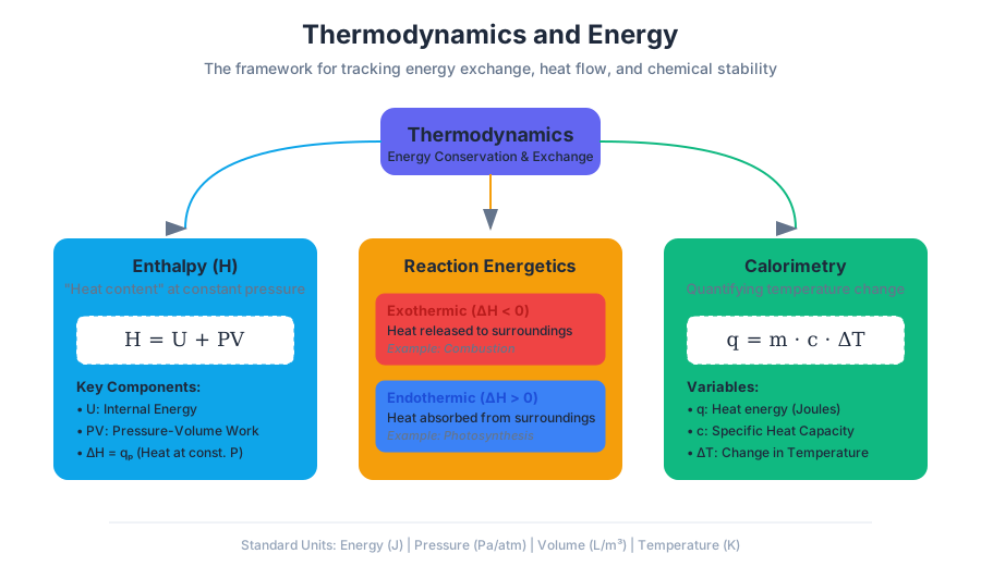
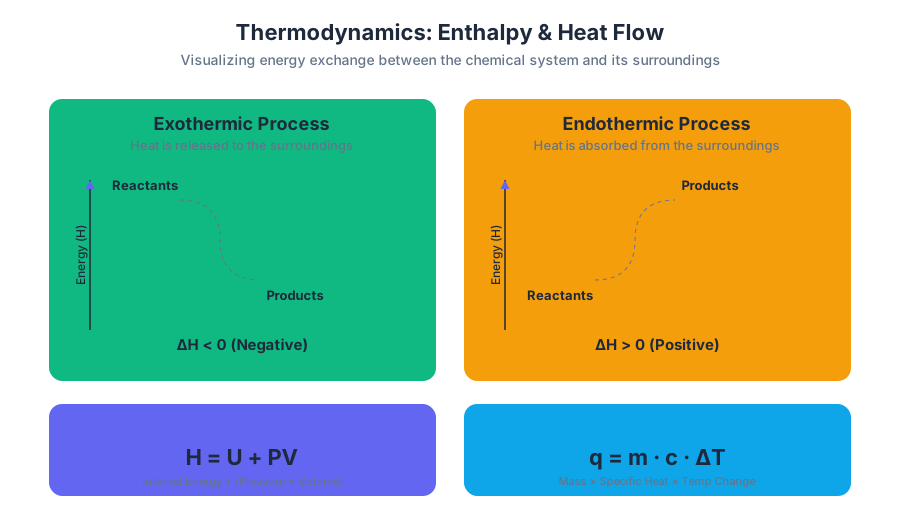
Nuclear Chemistry
Key concepts: Radioactive Decay · Fission vs. Fusion · Half-life · Alpha, Beta, and Gamma radiation
Advanced study of changes occurring within the nucleus of an atom.
Nuclear Chemistry
Nuclear chemistry is the study of transformations within the atomic nucleus. While traditional chemistry is governed by the behavior of valence electrons—dictated by the electromagnetic force—nuclear chemistry is dominated by the Strong Nuclear Force and the Weak Nuclear Force. The energy scales involved in nuclear transitions are typically six orders of magnitude greater than those in chemical reactions (Mega-electron volts [MeV] versus electron volts [eV]).
The Nature of Nuclear Stability
The stability of a nucleus is a delicate balance between the Strong Force (which attracts nucleons) and Electrostatic Repulsion (which pushes protons apart). For light elements, a 1:1 ratio of neutrons to protons ($N/Z = 1$) is generally stable. As the atomic number ($Z$) increases, an excess of neutrons is required to "dilute" the proton-proton repulsion, leading to a stable ratio of approximately 1.5:1 for the heaviest stable elements.
The Band of Stability: A graphical region representing the ratio of neutrons to protons that results in a stable nucleus. Nuclei outside this band are unstable and undergo radioactive decay to reach a lower energy, more stable state.
Binding Energy per Nucleon
The "mass defect" is the difference between the mass of a nucleus and the sum of the masses of its individual nucleons. This missing mass is converted into Nuclear Binding Energy according to Einstein’s equation $E=mc^2$.
| Feature | Chemical Reactions | Nuclear Reactions |
|---|---|---|
| Primary Actors | Valence Electrons | Protons and Neutrons (Nucleons) |
| Energy Change | Small (kJ/mol) | Massive (Millions of kJ/mol) |
| Conservation | Mass and Atoms conserved | Mass-Energy and Nucleons conserved |
| Influence | Temperature, Pressure, Catalysts | Independent of external conditions |
| Identity Change | Atoms rearranged into molecules | Elements change into different elements |
Radioactive Decay
Radioactive decay is a stochastic (random) process by which an unstable nucleus loses energy by emitting radiation. There are three primary modes of decay, each characterized by the type of particle or energy released.
Alpha ($\alpha$) Decay
In alpha decay, a nucleus ejects an alpha particle, which is essentially a Helium-4 nucleus ($^4_2\text{He}$). This occurs most frequently in heavy nuclei ($Z > 82$).
- Result: Atomic number decreases by 2; Mass number decreases by 4.
- Example: $^{238}{92}\text{U} \rightarrow ^{234}{90}\text{Th} + ^4_2\text{He}$
Beta ($\beta$) Decay
Beta decay involves the Weak Nuclear Force and comes in two primary forms:
- Beta-minus ($\beta^-$): A neutron transforms into a proton, an electron (the beta particle), and an antineutrino. This happens when the $N/Z$ ratio is too high.
- Beta-plus ($\beta^+$ or Positron Emission): A proton transforms into a neutron, a positron, and a neutrino. This happens when the $N/Z$ ratio is too low.
- Example ($\beta^-$): $^{14}_6\text{C} \rightarrow ^{14}_7\text{N} + e^- + \bar{\nu}_e$
Gamma ($\gamma$) Emission
Gamma decay is the emission of high-energy photons from an excited nucleus. It often follows alpha or beta decay when the daughter nucleus is left in a metastable state.
- Result: No change in atomic or mass number; only energy state changes.
Summary of Radiation Types
| Type | Symbol | Composition | Charge | Penetration Power | Shielding Required |
|---|---|---|---|---|---|
| Alpha | $\alpha$ | 2p, 2n | +2 | Very Low | Sheet of paper |
| Beta | $\beta$ | 1 electron | -1 | Moderate | Aluminum foil |
| Gamma | $\gamma$ | High-energy photon | 0 | Very High | Thick lead or concrete |
| Neutron | $n$ | 1 neutron | 0 | Extremely High | Water or paraffin |
Kinetics of Decay: Half-Life
Radioactive decay follows first-order kinetics. The rate of decay is proportional to the number of radioactive nuclei present.
The Mathematical Derivation
The rate law is expressed as: $$\frac{dN}{dt} = -\lambda N$$ Where $N$ is the number of nuclei and $\lambda$ is the decay constant.
\text{Integrating the rate law:} \\
\int_{N_0}^{N} \frac{dN}{N} = -\int_{0}^{t} \lambda dt \\
\ln\left(\frac{N}{N_0}\right) = -\lambda t \\
N(t) = N_0 e^{-\lambda t}
The Half-life ($t_{1/2}$) is the time required for $N$ to reach $N_0/2$. By substituting $N = N_0/2$ into the integrated rate law: $$\ln(0.5) = -\lambda t_{1/2}$$ $$t_{1/2} = \frac{\ln(2)}{\lambda} \approx \frac{0.693}{\lambda}$$
Worked Example: Carbon Dating
Suppose a wooden artifact is found to have a $^{14}\text{C}$ activity of 3.9 disintegrations per minute (dpm) per gram of carbon. Living wood has an activity of 15.6 dpm/g. Given $t_{1/2}$ for $^{14}\text{C}$ is 5,730 years, how old is the artifact?
- Find $\lambda$: $\lambda = 0.693 / 5730 \approx 1.21 \times 10^{-4} \text{ yr}^{-1}$
- Solve for $t$: $3.9 = 15.6 \cdot e^{-(1.21 \times 10^{-4})t}$
- $0.25 = e^{-(1.21 \times 10^{-4})t}$
- $\ln(0.25) = -(1.21 \times 10^{-4})t$
- $t \approx 11,460 \text{ years}$ (Exactly two half-lives).
Fission vs. Fusion
The Binding Energy Curve shows that Iron-56 ($^{56}\text{Fe}$) has the highest binding energy per nucleon, making it the most stable nucleus. Nuclei heavier than Iron can release energy by splitting (Fission), while nuclei lighter than Iron can release energy by joining (Fusion).
Nuclear Fission
Fission is the process where a heavy nucleus (like $^{235}\text{U}$) captures a neutron, becomes unstable, and splits into two smaller "fission fragments" and additional neutrons.
- Chain Reaction: If the emitted neutrons strike other fissile nuclei, a self-sustaining reaction occurs.
- Critical Mass: The minimum amount of fissile material needed to maintain a chain reaction.
Nuclear Fusion
Fusion is the process of combining light nuclei to form a heavier one. This powers stars via the Proton-Proton Chain or the CNO Cycle.
- The Challenge: Nuclei are positively charged and repel each other (Coulomb barrier). Fusion requires extreme temperatures (millions of degrees) to give nuclei enough kinetic energy to overcome this repulsion.
| Property | Nuclear Fission | Nuclear Fusion |
|---|---|---|
| Definition | Splitting heavy nuclei | Joining light nuclei |
| Fuel | Uranium, Plutonium | Hydrogen isotopes (Deuterium, Tritium) |
| Energy Yield | High | Extremely High (3-4x Fission) |
| Waste | Long-lived radioactive isotopes | Helium (Inert) |
| Status | Commercial power plants | Experimental (ITER, NIF) |
Technical Implementation: Modeling Decay
To understand the behavior of complex decay chains (where a parent decays to a daughter which is also radioactive), we use the Bateman Equations. Below is a low-level implementation in C for simulating a simple decay chain.
#include <stdio.h>
#include <math.h>

/**
 * Simulates a decay chain: A -> B -> C (stable)
 * Using Euler's method for numerical integration of the differential equations.
 */

typedef struct {
    double N_A; // Nuclei of species A
    double N_B; // Nuclei of species B
    double N_C; // Nuclei of species C
    double lambda_A;
    double lambda_B;
} DecaySystem;

void step_simulation(DecaySystem *sys, double dt) {
    double dNA = -sys->lambda_A * sys->N_A * dt;
    double dNB = (sys->lambda_A * sys->N_A - sys->lambda_B * sys->N_B) * dt;
    double dNC = (sys->lambda_B * sys->N_B) * dt;

    sys->N_A += dNA;
    sys->N_B += dNB;
    sys->N_C += dNC;
}

int main() {
    DecaySystem sys = {1000.0, 0.0, 0.0, 0.1, 0.05}; // Initial counts and constants
    double t = 0;
    double dt = 0.1;

    printf("Time\tSpecies_A\tSpecies_B\tSpecies_C\n");
    for (int i = 0; i <= 100; i++) {
        if (i % 10 == 0) {
            printf("%.1f\t%.2f\t\t%.2f\t\t%.2f\n", t, sys.N_A, sys.N_B, sys.N_C);
        }
        step_simulation(&sys, dt);
        t += dt;
    }
    return 0;
}
For higher-level analysis, such as determining the age of a sample based on isotopic ratios, Python with the NumPy library is the standard tool.
import numpy as np

def calculate_age(current_ratio, initial_ratio, half_life):
    """
    Calculates the age of a sample based on radioactive decay.
    Formula: t = (ln(N/N0) / -lambda)
    """
    decay_constant = np.log(2) / half_life
    age = np.log(current_ratio / initial_ratio) / -decay_constant
    return age

# Example: Potassium-Argon Dating
# 40K decays to 40Ar with a half-life of 1.25 billion years.
half_life_k40 = 1.25e9
current_k40_ratio = 0.125 # 1/8th of original remains
age = calculate_age(current_k40_ratio, 1.0, half_life_k40)

print(f"Sample Age: {age / 1e9:.2f} billion years")
# Output: Sample Age: 3.75 billion years
Common Pitfalls and Misconceptions
- Mass Conservation: Students often think mass is conserved in nuclear reactions. It is not. Mass-Energy is conserved. The "lost" mass is what provides the kinetic energy of the particles and the energy of the gamma rays.
- Half-life and Sample Size: A common mistake is thinking that a half-life means exactly half the atoms decay in that time. Because decay is a statistical process, this is only true for large populations. For a single atom, the half-life represents the time at which there is a 50% probability of decay.
- Radiation vs. Radioactivity: Radioactivity is the property of the nucleus (the "instability"). Radiation is the stuff that is emitted (particles or waves).
- Penetration vs. Ionization: There is an inverse relationship between penetration and ionization. Alpha particles have the lowest penetration but the highest Linear Energy Transfer (LET), meaning they do the most damage to biological tissue if ingested because they are highly ionizing.
Advanced Applications
Medical Isotopes and PET Scans
Positron Emission Tomography (PET) relies on $\beta^+$ decay. A patient is injected with a tracer like Fluorine-18 ($^{18}\text{F}$), which is incorporated into glucose. As the $^{18}\text{F}$ decays, it emits a positron. When this positron encounters an electron in the body, they annihilate, producing two gamma rays moving in opposite directions. Sensors detect these rays to map metabolic activity in the brain or tumors.
Nuclear Transmutation
Using particle accelerators, scientists can bombard stable nuclei with high-speed particles to create synthetic elements. This is how all transuranic elements (elements with $Z > 92$, like Americium used in smoke detectors) are produced.
# Example: Using a hypothetical CLI tool 'nuc-query' to check isotope properties
$ nuc-query info U-235
Isotope: Uranium-235
Mass: 235.0439 u
Abundance: 0.72%
Decay Mode: Alpha
Half-life: 7.04e8 years
Fissile: Yes (Thermal Neutrons)
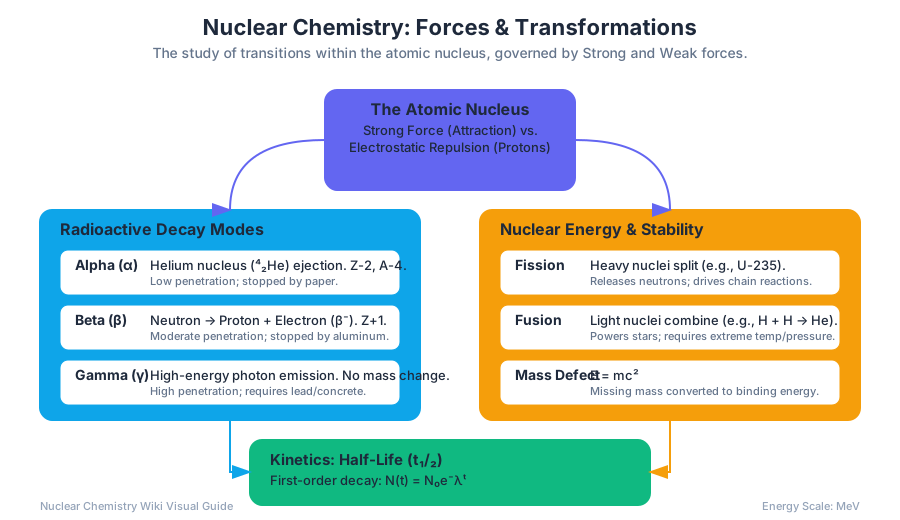
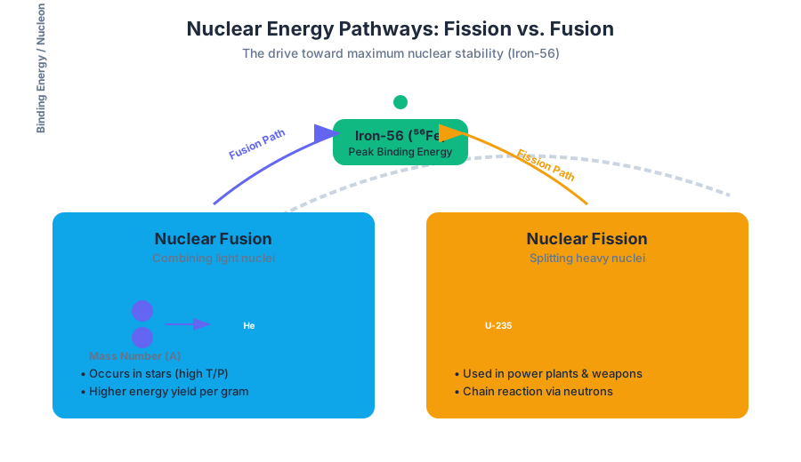
Source Materials
Study High School Chemistry with AI — Free on Lykke
Sign up for free to generate personalized flashcards, quizzes, and study guides from this course. Chat with an AI tutor that knows the material.
Get Started FreeView this course wiki on Lykke · Browse all public course wikis