High School Biology
Institution: MIT
42 study materials · 11 sections
The Client Challenge course is a comprehensive high school biology curriculum designed to guide students through the fundamental pillars of life sciences. The course spans from the molecular foundations of life and cellular mechanics to the complexities of genetics and biological reproduction. Students will engage with core concepts such as the scientific method, metabolic pathways, and the principles of heredity to build a robust understanding of how living organisms function and interact with their environment.
Course Sections
The Scientific Method and Experimental Design
Key concepts: Experimental design · Bias · Data analysis · Hypothesis testing
An introduction to the systematic approach used by biologists to explore the natural world.
The Scientific Method and Experimental Design
The scientific method is not merely a sequence of steps found in a middle-school textbook; it is a rigorous epistemological framework designed to minimize human error and maximize the reliability of our understanding of the natural world. In biology, where systems are characterized by high stochasticity and complex interdependencies, the application of this method requires a sophisticated grasp of experimental design, statistical inference, and bias mitigation.
The Epistemology of Inquiry: Beyond the Linear Model
At its core, the scientific method is an iterative cycle of falsification. As proposed by Karl Popper, a theory is only scientific if it is falsifiable—that is, there must be a conceivable observation that could prove it wrong. We do not "prove" hypotheses; we fail to reject them, thereby increasing our confidence in their validity.
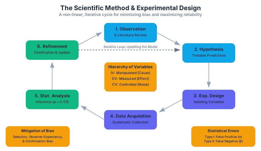
The modern scientific workflow follows a non-linear path:
- Observation and Literature Review: Identifying a phenomenon and situating it within existing theoretical frameworks.
- Hypothesis Formulation: Constructing a testable, predictive statement.
- Experimental Design: Engineering a controlled environment to isolate variables.
- Data Acquisition: Systematic collection of empirical evidence.
- Statistical Analysis: Determining the probability that observed effects are due to chance.
- Refinement: Updating the hypothesis based on results and repeating the cycle.
Experimental Design: The Architecture of Evidence
Experimental design is the process of planning a study to meet specified objectives while ensuring the data collected can be analyzed to yield valid and objective conclusions. In biological research, the primary challenge is confounding variables—uncontrolled factors that influence the outcome, leading to incorrect associations.
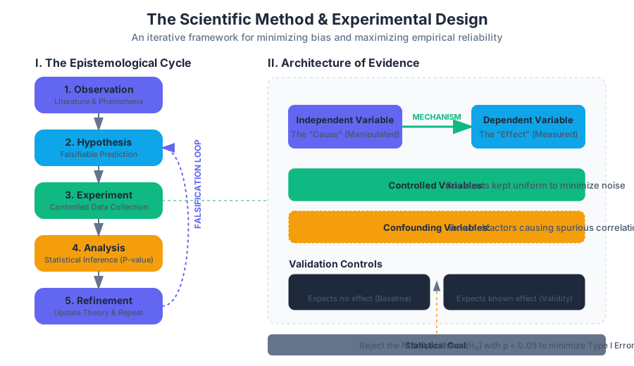
The Hierarchy of Variables
To isolate the mechanism of interest, we must strictly categorize the components of our experiment.
| Variable Type | Definition | Role in Experiment |
|---|---|---|
| Independent Variable (IV) | The factor manipulated by the researcher. | The hypothesized "Cause." |
| Dependent Variable (DV) | The factor being measured or observed. | The hypothesized "Effect." |
| Controlled Variables | Factors kept constant across all groups. | Minimizing "Noise" or Confounding. |
| Confounding Variable | An unmeasured third variable that influences both IV and DV. | The source of "Spurious Correlation." |
The Role of Controls
A "controlled experiment" is defined by the presence of comparison groups that allow the researcher to account for variables other than the one being tested.
- Negative Control: A group where no response is expected. This confirms that the experimental system is not producing false positives (e.g., treating a cell culture with a saline solution instead of a drug).
- Positive Control: A group where a known response is expected. This confirms that the experimental setup is capable of detecting an effect (e.g., treating a cell culture with a known toxin to ensure the cell-death assay is working).
The Gold Standard: Randomized Controlled Trials (RCTs) In clinical and high-level biological research, the RCT is the pinnacle of design. By randomly assigning subjects to groups, researchers ensure that both known and unknown confounding variables are distributed equally, isolating the effect of the independent variable.
Statistical Hypothesis Testing
Data analysis is the bridge between raw observations and scientific conclusions. We use Inferential Statistics to make generalizations about a population based on a sample.
The Null and Alternative Hypotheses
Mathematically, we frame our inquiry as a choice between two competing statements:
- Null Hypothesis ($H_0$): There is no effect or relationship (e.g., "Drug X does not affect heart rate").
- Alternative Hypothesis ($H_A$): There is a significant effect or relationship (e.g., "Drug X significantly increases heart rate").
The Logic of the P-Value
The $p$-value is the probability of obtaining results at least as extreme as the observed results, assuming the null hypothesis is true. It is a measure of "surprisal." If the $p$-value is low (typically $p < 0.05$), we reject the null hypothesis.
t = \frac{\bar{x}_1 - \bar{x}_2}{\sqrt{\frac{s_1^2}{n_1} + \frac{s_2^2}{n_2}}}
The formula for the t-statistic, used to compare the means of two groups. Here, $\bar{x}$ is the mean, $s^2$ is the variance, and $n$ is the sample size.
Type I and Type II Errors
No statistical test is perfect. We categorize errors based on whether we incorrectly rejected or failed to reject the null hypothesis.
| Decision | $H_0$ is True (No Effect) | $H_0$ is False (Real Effect) |
|---|---|---|
| Reject $H_0$ | Type I Error ($\alpha$) (False Positive) | Correct Decision (Power) |
| Fail to Reject $H_0$ | Correct Decision | Type II Error ($\beta$) (False Negative) |
Bias: The Silent Corruptor of Data
Bias is a systematic error that results in an incorrect estimate of the association between an exposure and an outcome. Unlike random error (noise), which decreases with larger sample sizes, bias is inherent in the design and cannot be "averaged out."
Common Forms of Bias in Biology
- Selection Bias: Occurs when the individuals included in the study are not representative of the target population.
- Observer-Expectancy Effect (Experimenter Bias): When a researcher’s cognitive bias causes them to subconsciously influence the participants or misinterpret data to fit their hypothesis.
- Confirmation Bias: The tendency to search for, interpret, and favor information that confirms one's pre-existing beliefs.
- Publication Bias: The tendency for journals to publish "positive" results ($p < 0.05$) while ignoring "negative" or null results, skewing the overall body of scientific literature.
Mitigation Strategies
To combat bias, researchers employ several rigorous techniques:
- Blinding: In a single-blind study, the subject does not know if they are in the control or experimental group. In a double-blind study, neither the subject nor the researcher collecting the data knows.
- Randomization: Using algorithmic randomness to assign subjects to groups.
- Placebos: Providing a sham treatment to account for the psychological effect of receiving "care."
Implementation: A Computational Approach to Analysis
In modern biology, data analysis is rarely done by hand. We use computational environments to process large datasets and perform statistical tests. Below is a Python implementation using SciPy and NumPy to simulate a controlled experiment and analyze the results.
import numpy as np
from scipy import stats

def run_experiment_simulation(n_samples=100, effect_size=0.5):
    """
    Simulates a controlled experiment comparing a Control group
    to an Experimental group.
    """
    # Generate synthetic data for Control (Mean=10, SD=2)
    control_group = np.random.normal(loc=10.0, scale=2.0, size=n_samples)

    # Generate synthetic data for Experimental (Mean=10 + effect_size, SD=2)
    experimental_group = np.random.normal(loc=10.0 + effect_size, scale=2.0, size=n_samples)

    # Perform Welch's t-test (does not assume equal variance)
    t_stat, p_val = stats.ttest_ind(control_group, experimental_group, equal_var=False)

    return {
        "control_mean": np.mean(control_group),
        "exp_mean": np.mean(experimental_group),
        "t_statistic": t_stat,
        "p_value": p_val
    }

# Execute simulation
results = run_experiment_simulation(n_samples=50, effect_size=1.2)
print(f"P-Value: {results['p_value']:.4f}")
if results['p_value'] < 0.05:
    print("Result: Statistically Significant. Reject Null Hypothesis.")
else:
    print("Result: Not Significant. Fail to Reject Null Hypothesis.")
While Python is excellent for simulation, the R language remains the standard for complex biological statistical modeling due to its robust library ecosystem (like ggplot2 for visualization and lme4 for mixed-effects models).
# R Script: Linear Modeling of Plant Growth
# Hypothesis: Nitrogen concentration affects stem height

# Load dataset
data <- read.csv("plant_growth_data.csv")

# Fit a linear model: Height as a function of Nitrogen concentration
model <- lm(height ~ nitrogen_conc, data = data)

# Generate Summary Statistics
summary(model)

# Visualization with Confidence Intervals
library(ggplot2)
ggplot(data, aes(x=nitrogen_conc, y=height)) +
  geom_point() +
  geom_smooth(method="lm", col="blue") +
  labs(title="Plant Height vs Nitrogen Concentration",
       x="Nitrogen (mg/L)", y="Height (cm)")
Advanced Concepts: Power and Effect Size
A common pitfall in experimental design is focusing solely on the $p$-value while ignoring Effect Size and Statistical Power.
- Effect Size: A quantitative measure of the magnitude of the experimental effect (e.g., Cohen's $d$). A result can be statistically significant but biologically irrelevant if the effect size is tiny.
- Statistical Power ($1 - \beta$): The probability that a test will correctly reject a false null hypothesis. Power is influenced by sample size ($n$), effect size, and the significance level ($\alpha$).
Worked Example: Sample Size Calculation If a researcher wants to detect a medium effect size ($d = 0.5$) with 80% power at a significance level of 0.05, they would need approximately 64 participants per group. If they only use 20 participants, their power drops significantly, increasing the risk of a Type II error (failing to find a real effect).
The Replication Crisis and Open Science
In recent years, the scientific community has faced a "replication crisis," where many landmark studies (particularly in psychology and medicine) have failed to produce the same results when repeated. This has led to a shift toward Open Science practices:
- Pre-registration: Researchers submit their hypothesis and analysis plan to a public registry before conducting the experiment to prevent "p-hacking" (manipulating data until a significant result is found).
- Data Sharing: Making raw data available for independent verification.
- Replication Studies: Explicitly funding and publishing studies that attempt to reproduce previous findings.
Summary of Best Practices
To ensure the integrity of biological research, the following principles must be adhered to:
| Principle | Actionable Step |
|---|---|
| Objectivity | Use double-blinding whenever human subjects or observers are involved. |
| Reproducibility | Document all protocols, reagents (including catalog numbers), and software versions. |
| Transparency | Report all data, including outliers and "failed" experiments. |
| Rigorous Analysis | Use appropriate statistical tests based on data distribution (e.g., non-parametric tests for non-normal data). |
Chemical Foundations: Water and pH
Key concepts: Hydrogen bonding · Density of ice · Thermal insulation · pH scale · Acids and bases
Exploring the unique properties of water and the importance of pH balance in biological systems.
Chemical Foundations: Water and pH
Life, as we understand it, is not merely supported by water; it is fundamentally written in the language of aqueous chemistry. From the folding of complex proteins to the maintenance of electrochemical gradients across cell membranes, the physical and chemical properties of water dictate the boundary conditions of biology. This section explores the molecular architecture of water, the anomalous behavior of its solid phase, and the logarithmic scale of pH that governs enzymatic activity and homeostasis.
The Molecular Architecture of Water: Hydrogen Bonding
At the heart of water’s unique behavior is its polarity. A single water molecule ($H_2O$) consists of one oxygen atom covalently bonded to two hydrogen atoms. However, these bonds are polar covalent. Oxygen, being highly electronegative, exerts a stronger pull on the shared electrons than the hydrogen atoms.
What it is
Hydrogen Bonding is a specific type of dipole-dipole attraction that occurs when a hydrogen atom, covalently bonded to a highly electronegative atom (like Oxygen), experiences the electrostatic pull of a lone pair of electrons on a neighboring electronegative atom.
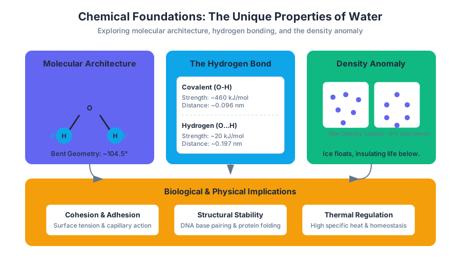
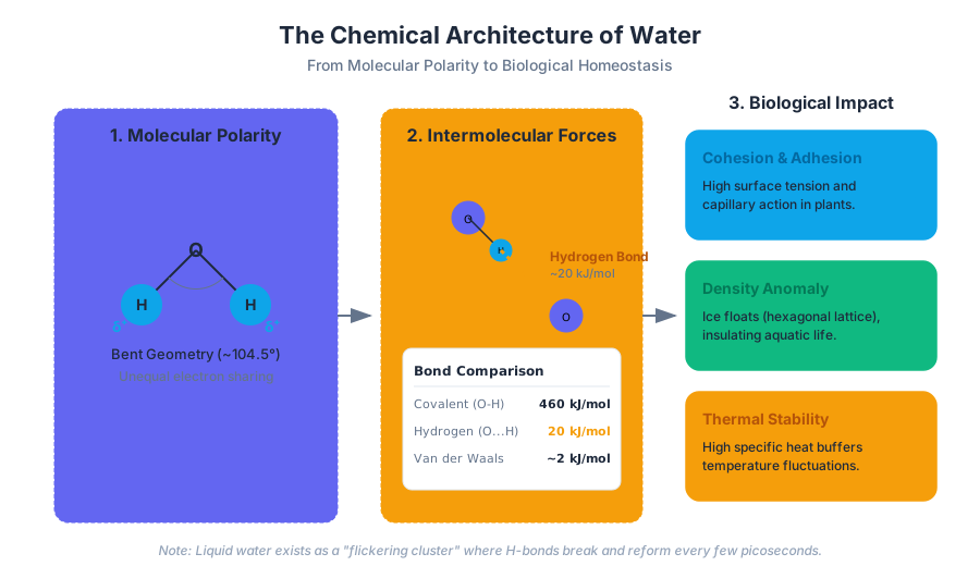
Definition: The Hydrogen Bond A non-covalent interaction where a hydrogen atom serves as a bridge between two electronegative atoms. In water, the bond energy is approximately 20 kJ/mol—significantly weaker than a covalent O-H bond (~460 kJ/mol) but strong enough to confer structural stability to liquid water.
Why it matters
Without hydrogen bonding, water would be a gas at room temperature (similar to hydrogen sulfide, $H_2S$). These bonds are responsible for cohesion (water sticking to itself), adhesion (water sticking to other surfaces), and the high surface tension that allows certain insects to walk on ponds. In a biological context, hydrogen bonds hold the two strands of the DNA double helix together and are the primary force behind protein secondary structures (alpha-helices and beta-sheets).
How it works: The Dipole Moment
The geometry of water is "bent" (approximately 104.5°) due to the two lone pairs of electrons on the oxygen atom. This asymmetry, combined with the electronegativity difference, creates a molecular dipole where the oxygen side is partially negative ($\delta^-$) and the hydrogen side is partially positive ($\delta^+$).
| Property | Covalent Bond (O-H) | Hydrogen Bond (O...H) | Van der Waals Forces |
|---|---|---|---|
| Type | Intramolecular | Intermolecular | Intermolecular |
| Strength | Very Strong (~460 kJ/mol) | Moderate (~20 kJ/mol) | Weak (~1-4 kJ/mol) |
| Distance | Short (~0.096 nm) | Longer (~0.197 nm) | Variable |
| Role | Holds the molecule together | Creates fluid networks | General atomic attraction |
Concrete Example: Simulating Dipole Interactions
To understand the strength of these interactions in a computational context, we can model the potential energy of a dipole-dipole interaction.
import numpy as np

def calculate_dipole_potential(mu1, mu2, r, theta1, theta2, phi):
    """
    Calculates the potential energy (V) between two dipoles.
    mu: Dipole moments
    r: Distance between centers
    theta/phi: Orientation angles in radians
    """
    # Vacuum permittivity constant (simplified for demonstration)
    epsilon_0 = 8.854e-12
    k = 1 / (4 * np.pi * epsilon_0)

    # Simplified formula for collinear dipoles
    term1 = np.cos(theta1) * np.cos(theta2)
    term2 = np.sin(theta1) * np.sin(theta2) * np.cos(phi)

    v = (k * mu1 * mu2 / r**3) * (term1 - 0.5 * term2)
    return v

# Example: Two water molecules at 0.3nm distance
water_mu = 1.85 * 3.335e-30  # Debye to Coulomb-meters
energy = calculate_dipole_potential(water_mu, water_mu, 0.3e-9, 0, 0, 0)
print(f"Potential Energy: {energy:.2e} Joules")
Common Pitfalls
A frequent misconception is that hydrogen bonds are "real" bonds like covalent ones. They are actually electrostatic attractions. Another error is assuming water only forms four hydrogen bonds in a static way. In reality, liquid water is a "flickering cluster" where bonds break and reform every few picoseconds.
The Density Anomaly and Thermal Insulation
Most substances follow a simple rule: the solid phase is denser than the liquid phase because molecules pack more tightly as kinetic energy decreases. Water is a defiant exception.
What it is
The Density Anomaly refers to the fact that water reaches its maximum density at 4°C (39.2°F). As it cools further toward 0°C, it begins to expand. Upon freezing, it undergoes a phase transition into a crystalline lattice that is roughly 9% less dense than liquid water.
Why it matters: The Survival of Aquatic Ecosystems
If ice were denser than liquid water, lakes and oceans would freeze from the bottom up. During winter, the entire body of water would eventually turn into a solid block of ice, killing all complex life. Because ice floats, it creates a surface layer of thermal insulation. This layer traps the heat of the liquid water below, keeping it at a relatively stable temperature (usually around 4°C at the bottom) and allowing fish and plants to survive the winter.
How it works: The Hexagonal Lattice
In liquid water, molecules are crowded together, constantly shifting. As water freezes, the hydrogen bonds become stable and force the molecules into a hexagonal crystal lattice. In this arrangement, each oxygen atom is at the center of a tetrahedron of four hydrogen atoms. This geometry requires more space than the disordered liquid state, resulting in an increase in volume and a decrease in density.
| State of Water | Temperature (°C) | Density (g/cm³) | Molecular Arrangement |
|---|---|---|---|
| Liquid | 100 | 0.9584 | Highly disordered, rapid motion |
| Liquid | 4 | 1.0000 | Maximum packing efficiency |
| Liquid | 0 | 0.9998 | Beginning of lattice formation |
| Solid (Ice) | 0 | 0.9167 | Rigid, open hexagonal lattice |
Concrete Example: The Clausius-Clapeyron Relation
The relationship between pressure and the freezing point of water is described by the Clausius-Clapeyron equation. Because ice is less dense than water, increasing pressure actually lowers the melting point—a phenomenon called regelation.
\frac{dP}{dT} = \frac{L}{T \Delta V}
Where:
- $L$ is the latent heat of fusion.
- $T$ is the temperature.
- $\Delta V$ is the change in molar volume ($V_{liquid} - V_{solid}$).
- Since $\Delta V$ is negative for water, the slope $dP/dT$ is negative.
Variations: Heavy Water ($D_2O$)
In "heavy water," the hydrogen atoms are replaced by deuterium. $D_2O$ is about 11% denser than normal water and has a slightly higher freezing point (3.82°C). Interestingly, while chemically similar, high concentrations of heavy water are toxic to eukaryotic organisms because they disrupt the delicate timing of mitosis.
The pH Scale and Auto-ionization
The chemical reactivity of water is defined by its ability to dissociate into ions. This self-ionization is the foundation of the pH scale.
What it is
The pH scale is a logarithmic measure of the molar concentration of hydrogen ions ($H^+$) in a solution. Since $H^+$ ions do not exist freely in water but rather associate with water molecules to form hydronium ($H_3O^+$), pH is technically a measure of hydronium activity.
The pH Equation $$pH = -\log_{10}[H^+]$$ In pure water at 25°C, $[H^+] = 1.0 \times 10^{-7} M$, resulting in a pH of 7.0.
Why it matters
Biological systems are extremely sensitive to pH. Human blood must be maintained within a narrow window (7.35 to 7.45). A shift of even 0.5 units can lead to coma or death. This is because the charge of amino acid side chains in proteins changes with pH, which in turn alters the protein's shape and function (denaturation).
How it works: The Ion Product of Water ($K_w$)
Water undergoes auto-ionization according to the following equilibrium:
H_2O + H_2O \rightleftharpoons H_3O^+ + OH^-
The equilibrium constant for this reaction, known as $K_w$, is constant at a given temperature. At 25°C: $$K_w = [H^+][OH^-] = 1.0 \times 10^{-14}$$
Derivation of the Scale
If we take the negative logarithm of both sides of the $K_w$ expression: $$-\log(K_w) = -\log([H^+][OH^-])$$ $$pK_w = pH + pOH = 14$$
This relationship ensures that as the concentration of hydrogen ions increases (acidic), the concentration of hydroxide ions must decrease proportionally.
| Solution Type | $[H^+]$ (M) | pH | $[OH^-]$ (M) | pOH |
|---|---|---|---|---|
| Strongly Acidic | $10^0$ | 0 | $10^{-14}$ | 14 |
| Gastric Acid | $10^{-2}$ | 2 | $10^{-12}$ | 12 |
| Neutral Water | $10^{-7}$ | 7 | $10^{-7}$ | 7 |
| Bleach | $10^{-12}$ | 12 | $10^{-2}$ | 2 |
| Strongly Basic | $10^{-14}$ | 14 | $10^0$ | 0 |
Concrete Example: Calculating pH of a Strong Acid
If you add 0.01 moles of Hydrochloric Acid ($HCl$) to 1 liter of water, what is the pH? Since $HCl$ is a strong acid, it dissociates completely.
/**
 * Simple pH Calculator for Strong Acids/Bases
 * @param {number} concentration - Molarity (M)
 * @param {string} type - 'acid' or 'base'
 * @returns {number} ph
 */
function calculatePH(concentration, type) {
    if (concentration <= 0) return 7.0;

    const pValue = -Math.log10(concentration);

    if (type === 'acid') {
        return parseFloat(pValue.toFixed(2));
    } else if (type === 'base') {
        return parseFloat((14 - pValue).toFixed(2));
    }
    return 7.0;
}

console.log(`pH of 0.01M HCl: ${calculatePH(0.01, 'acid')}`); // Output: 2
Acids, Bases, and Biological Buffers
While strong acids dissociate completely, most biological molecules are weak acids or weak bases, meaning they only partially dissociate in water.
What it is
- Brønsted-Lowry Acid: A substance that donates a proton ($H^+$).
- Brønsted-Lowry Base: A substance that accepts a proton.
- Buffer: A solution consisting of a weak acid and its conjugate base that resists changes in pH when small amounts of acid or base are added.
How it works: The Henderson-Hasselbalch Equation
The behavior of buffers is governed by the Henderson-Hasselbalch equation, which relates pH to the acid dissociation constant ($pK_a$) and the ratio of conjugate base to acid.
$$pH = pK_a + \log_{10}\left(\frac{[A^-]}{[HA]}\right)$$
When the concentration of the acid $[HA]$ equals the concentration of the conjugate base $[A^-]$, the $pH = pK_a$. This is the point where the buffer is most effective at resisting change.
Concrete Example: The Bicarbonate Buffer System
The human body manages blood pH primarily through the bicarbonate system:
CO_2 + H_2O \rightleftharpoons H_2CO_3 \rightleftharpoons HCO_3^- + H^+
If blood becomes too acidic, the equilibrium shifts to the left, and the excess $H^+$ is converted into $CO_2$, which is then exhaled by the lungs. If blood becomes too basic, the kidneys excrete more $HCO_3^-$ (bicarbonate) in the urine.
Common Pitfalls: The "Neutral" Misconception
A common mistake is thinking that "neutral" always means pH 7.0. The neutral point is defined as $[H^+] = [OH^-]$. Because $K_w$ changes with temperature, the neutral pH of water at 37°C (human body temperature) is actually approximately 6.8, not 7.0.
Real-World Usage: Querying Chemical Properties
In a laboratory or engineering setting, one might use a CLI tool or database to retrieve $pK_a$ values for buffer preparation.
# Hypothetical 'chemdb' CLI usage to find buffer properties
$ chemdb search "HEPES" --property pka
> Name: HEPES (4-(2-hydroxyethyl)-1-piperazineethanesulfonic acid)
> pKa at 25C: 7.55
> Useful pH range: 6.8 - 8.2
> Delta pKa / Delta T: -0.014 / C

# Calculate amount of salt needed for 1L of 0.1M HEPES at pH 7.4
$ chemdb buffer-calc --molarity 0.1 --target-ph 7.4 --acid "HEPES"
> Add 23.83g HEPES (Free Acid)
> Add 0.042 moles NaOH to adjust pH
Summary of Chemical Foundations
Water is the "Universal Solvent" not because it dissolves everything, but because its polar nature and hydrogen-bonding capacity allow it to interact with a vast array of biological molecules. Its thermal properties provide a stable environment for life, and its ionization provides the chemical landscape (pH) in which metabolism occurs.
| Concept | Key Takeaway | Biological Impact |
|---|---|---|
| Hydrogen Bonding | Polar attraction between $H$ and $O$. | Stabilizes DNA and protein structures. |
| Density Anomaly | Ice is less dense than liquid water. | Prevents lakes from freezing solid. |
| Specific Heat | Water absorbs high energy with low temp change. | Regulates body and environmental temperature. |
| pH Scale | Logarithmic measure of $[H^+]$. | Controls enzyme activity and reaction rates. |
| Buffers | Mixtures that resist pH shifts. | Maintains blood homeostasis. |
Biological Macromolecules
Key concepts: Carbohydrates · Proteins · Lipids · Nucleic acids
A deep dive into the four major classes of organic molecules that make up living organisms.
Biological Macromolecules
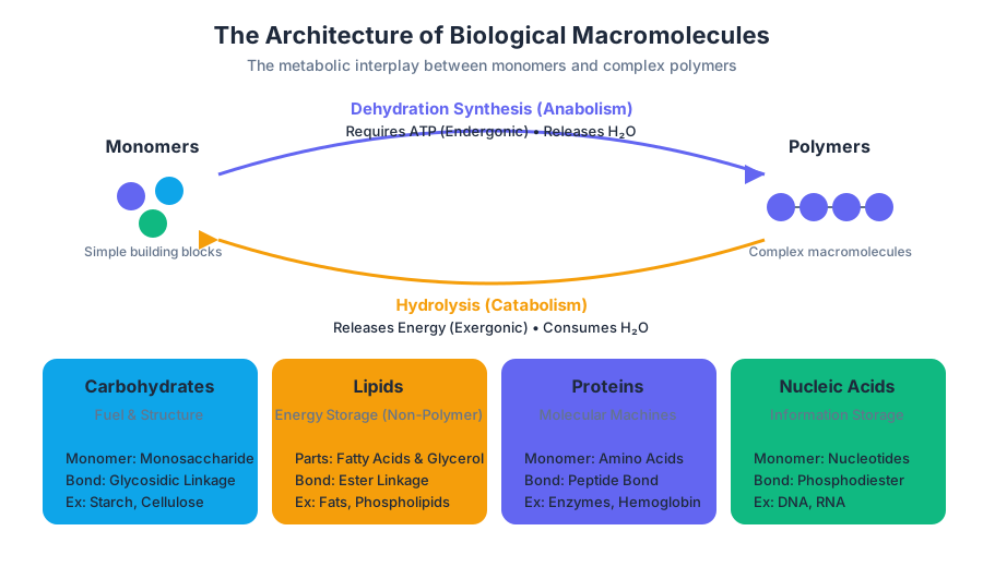
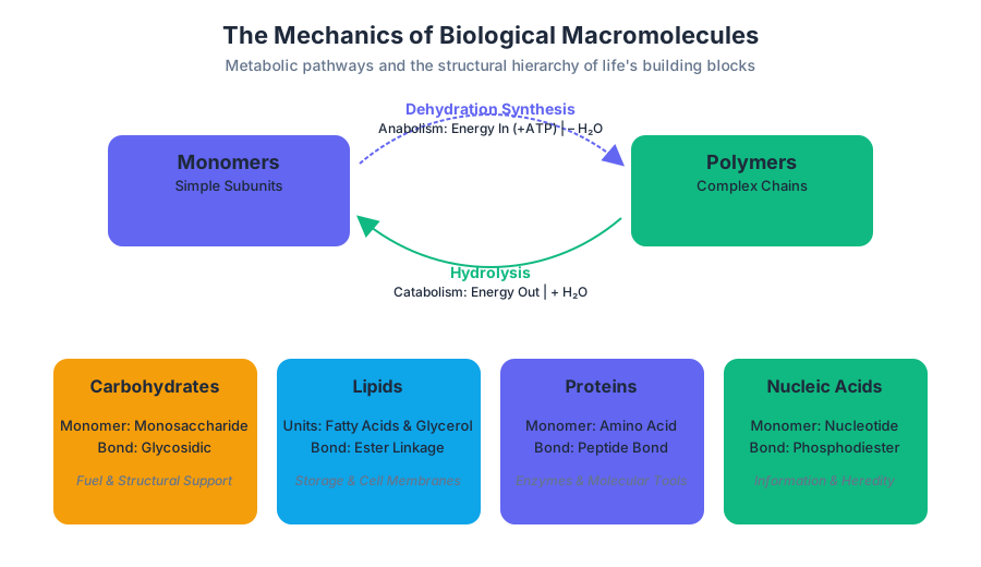
The architecture of life is built upon a foundation of four primary classes of organic compounds: Carbohydrates, Lipids, Proteins, and Nucleic Acids. These "macromolecules" are large, complex polymers synthesized from smaller, repeating units called monomers. The assembly and disassembly of these structures are governed by the laws of thermodynamics and the specific chemistry of the carbon atom.
Understanding biological macromolecules requires moving beyond simple definitions and into the realm of molecular mechanics. We must examine how covalent bonds are formed through dehydration synthesis, how they are cleaved via hydrolysis, and how the resulting three-dimensional conformations dictate the functional limits of a cell.
The Chemical Engine: Polymerization and Metabolism
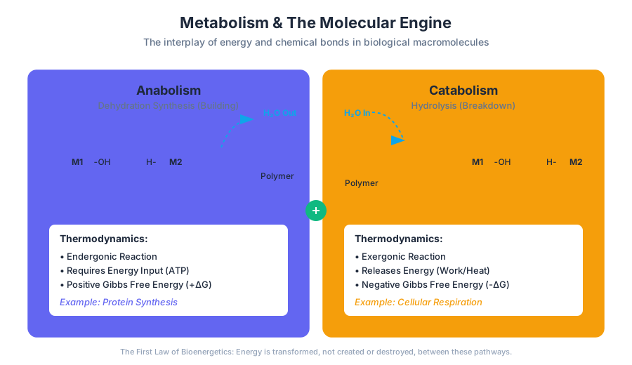
Before diving into specific classes, we must define the universal mechanism of macromolecular construction. Most biological polymers are formed through dehydration synthesis (also known as condensation reactions), where the hydrogen of one monomer combines with the hydroxyl group of another, releasing a water molecule ($H_2O$) and forming a covalent bond.
Conversely, the breakdown of these polymers occurs via hydrolysis, where a water molecule is consumed to bridge the gap between monomers, effectively "lysing" the bond. This interplay is the basis of metabolism, which is divided into two distinct pathways:
- Anabolism: The synthesis of complex molecules from simpler ones. These are endergonic reactions, meaning they require an input of energy (usually in the form of ATP).
- Catabolism: The breakdown of complex molecules into simpler ones. These are exergonic reactions, releasing energy that the cell can capture to perform work.
The First Law of Bioenergetics: Energy cannot be created or destroyed within a biological system, only transformed. The synthesis of a protein (anabolism) is fueled by the breakdown of glucose (catabolism), ensuring a continuous flow of Gibbs Free Energy ($\Delta G$) to maintain homeostasis.
| Process | Energy Change | Reaction Type | Example |
|---|---|---|---|
| Anabolism | Positive $\Delta G$ (Requires Energy) | Endergonic | Gluconeogenesis, Protein Synthesis |
| Catabolism | Negative $\Delta G$ (Releases Energy) | Exergonic | Glycolysis, Cellular Respiration |
| Dehydration | Bond Formation | Synthesis | Building Starch from Glucose |
| Hydrolysis | Bond Cleavage | Decomposition | Digestion of Dietary Proteins |
Carbohydrates: The Molecular Fuel and Scaffold
Carbohydrates are organic molecules composed of carbon, hydrogen, and oxygen, typically in a molar ratio of $1:2:1$, represented by the empirical formula $(CH_2O)_n$. They serve as the primary short-term energy source for cells and provide structural integrity to plants, fungi, and arthropods.
Monosaccharides and Disaccharides
The simplest carbohydrates are monosaccharides (e.g., glucose, fructose, galactose). In aqueous solutions, these often exist as cyclic structures. When two monosaccharides link via a glycosidic bond, they form a disaccharide (e.g., sucrose, lactose).
The orientation of the hydroxyl group on the anomeric carbon (the carbon derived from the carbonyl group) determines whether the bond is $\alpha$ (alpha) or $\beta$ (beta). This distinction is biologically critical: humans possess enzymes to digest $\alpha$-glycosidic bonds (starch) but lack the enzymes to break $\beta$-glycosidic bonds (cellulose).
Polysaccharides: Storage vs. Structure
Polysaccharides are long chains of monosaccharides. Their function is determined by their branching and the type of glycosidic linkage:
- Storage Polysaccharides: Starch (in plants) and Glycogen (in animals) are composed of $\alpha$-glucose. Glycogen is highly branched, allowing for rapid mobilization of glucose during exercise or fasting.
- Structural Polysaccharides: Cellulose (plant cell walls) and Chitin (fungal cell walls and arthropod exoskeletons) are composed of $\beta$-linkages, creating rigid, unbranched fibrils that are incredibly resistant to mechanical stress.
# Python implementation: Calculating the molecular weight of a polysaccharide
# This script accounts for the loss of H2O during dehydration synthesis.

def calculate_polymer_mass(monomer_mass, n_units):
    """
    Calculates the mass of a polymer chain.
    Formula: (monomer_mass * n) - (water_mass * (n - 1))
    """
    WATER_MASS = 18.015
    if n_units < 1:
        return 0

    total_mass = (monomer_mass * n_units) - (WATER_MASS * (n_units - 1))
    return round(total_mass, 3)

# Example: A chain of 100 Glucose molecules (C6H12O6, mass ~180.16)
glucose_mass = 180.156
chain_length = 100
print(f"Mass of {chain_length}-unit starch chain: {calculate_polymer_mass(glucose_mass, chain_length)} Da")
Lipids: Hydrophobicity and Energy Density
Unlike the other three macromolecules, lipids are not true polymers. They are a heterogeneous group of non-polar, hydrophobic compounds. Their primary roles include long-term energy storage, insulation, and forming the core of biological membranes.
Fatty Acids and Triacylglycerols
A fatty acid consists of a long hydrocarbon chain attached to a carboxyl group.
- Saturated Fatty Acids: Contain no double bonds between carbon atoms. They are "saturated" with hydrogen, allowing them to pack tightly and remain solid at room temperature (e.g., butter).
- Unsaturated Fatty Acids: Contain one or more double bonds, creating "kinks" in the chain. These kinks prevent tight packing, making them liquid at room temperature (e.g., vegetable oil).
Phospholipids and the Membrane
Phospholipids are the most important lipids for cellular structure. They are amphipathic, possessing a hydrophilic (polar) head and two hydrophobic (non-polar) tails. In water, they spontaneously organize into a lipid bilayer, the fundamental structure of the cell membrane.
The Fluid Mosaic Model: The cell membrane is not a static wall but a dynamic, fluid environment where proteins and lipids move laterally. The "fluidity" is regulated by the ratio of saturated to unsaturated fats and the presence of cholesterol, which acts as a temperature buffer.
| Lipid Type | Structure | Primary Function |
|---|---|---|
| Triglycerides | Glycerol + 3 Fatty Acids | Long-term energy storage (Adipose) |
| Phospholipids | Glycerol + 2 Fatty Acids + Phosphate | Membrane structure |
| Steroids | Four fused carbon rings | Signaling (Hormones) and Membrane fluidity |
| Waxes | Long-chain alcohol + Fatty acid | Protection and water-proofing |
Proteins: The Molecular Machines
Proteins are the most versatile macromolecules, accounting for more than 50% of the dry mass of most cells. They function as enzymes, structural supports, transporters, and signaling molecules.
Amino Acids: The Building Blocks
Proteins are polymers of amino acids. Each amino acid has a central carbon ($\alpha$-carbon) bonded to an amino group ($NH_2$), a carboxyl group ($COOH$), a hydrogen atom, and a variable R-group (side chain). There are 20 standard amino acids, categorized by the chemical properties of their R-groups: polar, non-polar, acidic, or basic.
The Four Levels of Protein Structure
The function of a protein is entirely dependent on its three-dimensional shape. This shape is achieved through four levels of organization:
- Primary (1°): The unique sequence of amino acids in the polypeptide chain, determined by genetic information.
- Secondary (2°): Localized folding patterns, such as $\alpha$-helices and $\beta$-pleated sheets, stabilized by hydrogen bonds between the polypeptide backbone.
- Tertiary (3°): The overall 3D shape of a single polypeptide, stabilized by interactions between R-groups (hydrophobic interactions, van der Waals forces, hydrogen bonds, ionic bonds, and disulfide bridges).
- Quaternary (4°): The structure resulting from the aggregation of two or more polypeptide subunits (e.g., Hemoglobin).
\text{Gibbs Free Energy of Folding: } \Delta G_{folding} = \Delta H_{folding} - T\Delta S_{folding}
For a protein to fold spontaneously, $\Delta G$ must be negative. While the decrease in entropy ($\Delta S$) of the protein itself is unfavorable, the "hydrophobic effect"—the increase in entropy of the surrounding water molecules—drives the process forward.
Enzymes and Activation Energy
Enzymes are protein catalysts that speed up biochemical reactions by lowering the activation energy ($E_a$). They do not change the $\Delta G$ of a reaction; they simply provide a pathway for the reaction to occur more rapidly.
// Conceptual representation of Enzyme-Substrate kinetics (Michaelis-Menten)
const enzymeKinetics = {
    vMax: 100, // Maximum velocity
    Km: 5,     // Michaelis constant (substrate concentration at 1/2 vMax)

    calculateRate: function(substrateConcentration) {
        // Michaelis-Menten Equation: v = (Vmax * [S]) / (Km + [S])
        return (this.vMax * substrateConcentration) / (this.Km + substrateConcentration);
    }
};

console.log(`Reaction rate at [S]=5: ${enzymeKinetics.calculateRate(5)}`);
// Output: 50 (which is 1/2 of vMax)
Nucleic Acids: Information Storage and Transfer
Nucleic Acids (DNA and RNA) are the polymers responsible for storing, transmitting, and expressing genetic information. They are composed of monomers called nucleotides.
Nucleotide Structure
Each nucleotide consists of three components:
- A Pentose Sugar (Deoxyribose in DNA, Ribose in RNA).
- A Phosphate Group.
- A Nitrogenous Base (Adenine, Guanine, Cytosine, Thymine in DNA, or Uracil in RNA).
Nucleotides are linked by phosphodiester bonds between the 5' phosphate of one nucleotide and the 3' hydroxyl group of the next, creating a sugar-phosphate backbone with a distinct directionality ($5' \to 3'$).
DNA vs. RNA
DNA serves as the long-term "hard drive" of the cell, existing as a double-stranded helix held together by hydrogen bonds between complementary bases (A-T, G-C). RNA is typically single-stranded and acts as a "temporary copy" (mRNA), a structural component (rRNA), or an adapter (tRNA) to translate genetic code into proteins.
| Feature | DNA (Deoxyribonucleic Acid) | RNA (Ribonucleic Acid) |
|---|---|---|
| Sugar | Deoxyribose | Ribose |
| Bases | A, G, C, T | A, G, C, U |
| Structure | Double-stranded Helix | Usually single-stranded |
| Stability | Highly stable (Long-term) | Relatively unstable (Short-term) |
| Location | Nucleus (Eukaryotes) | Nucleus and Cytoplasm |
# Bioinformatics: Using CLI to analyze a DNA sequence file (FASTA)
# Counting the occurrence of each nucleotide in a sequence

cat sequence.fasta | grep -v ">" | fold -w1 | sort | uniq -c

# Output example:
# 450 A
# 320 C
# 315 G
# 445 T
Integration: Gluconeogenesis and Metabolic Flux
To see these macromolecules in action, consider Gluconeogenesis. This is a metabolic pathway where the body synthesizes glucose (a carbohydrate) from non-carbohydrate precursors like pyruvate, lactate, or certain amino acids (derived from proteins).
This process is the reverse of glycolysis but is not a simple mirror image. It requires bypassing three irreversible steps of glycolysis using different enzymes. This is a classic example of anabolism:
- Energy Input: It consumes 4 ATP, 2 GTP, and 2 NADH to produce one molecule of glucose.
- Regulation: It is stimulated by the hormone glucagon when blood glucose levels are low, ensuring the brain has a constant fuel supply even during starvation.
Insight: The ability of a cell to switch between breaking down macromolecules (catabolism) and building them (anabolism) is what allows for homeostasis. If you consume excess protein, your body doesn't just store it as protein; it deaminates the amino acids and converts the carbon skeletons into lipids for long-term storage.
Common Pitfalls and Misconceptions
- "Lipids are polymers": This is technically false. While they are large molecules, they are not made of repeating monomeric units linked in a chain like proteins or carbohydrates.
- "All enzymes are proteins": Most are, but ribozymes (catalytic RNA molecules) prove that nucleic acids can also perform enzymatic work.
- "Saturated fats are 'bad'": Biologically, saturation is about membrane fluidity and energy density. The "health" aspect is a matter of dietary balance and physiological context, not a fundamental property of the molecule itself.
- "DNA is the only genetic material": While true for cellular life, many viruses use RNA as their primary genetic storage medium.
Cell Theory and Cellular Classification
Key concepts: Cell theory · Prokaryotic cells · Eukaryotic cells · Structural complexity
Understanding the fundamental unit of life and the distinctions between prokaryotic and eukaryotic cells.
Cell Theory and Cellular Classification
The cell is the fundamental unit of biological existence, representing the smallest scale at which the properties of life—metabolism, reproduction, and homeostasis—fully manifest. In the hierarchy of biological organization, the cell serves as the bridge between the stochastic world of molecular chemistry and the deterministic world of organismal physiology. Understanding cellular classification is not merely an exercise in taxonomy; it is an exploration of the physical and energetic constraints that dictate how life scales from single-celled bacteria to complex multicellular eukaryotes.
The Foundations of Cell Theory
Cell theory is the unifying principle of biology, providing a framework for understanding how life is structured and how it persists across generations. It emerged in the mid-19th century through the synthesis of microscopic observations and experimental evidence, effectively dismantling the long-held doctrine of spontaneous generation.
The Three Classical Tenets
The classical cell theory is defined by three core principles:
- The cell is the basic unit of structure and function in living things. No smaller subunit of an organism can independently perform all functions of life.
- All living organisms are composed of one or more cells. This applies to everything from the simplest unicellular prokaryote to the trillions of cells in a human body.
- All cells arise from pre-existing cells. This tenet, famously articulated by Rudolf Virchow as omnis cellula e cellula, establishes the continuity of life through cellular division.
The Modern Synthesis of Cell Theory
As our understanding of molecular biology matured, the theory expanded to include the chemical and genetic underpinnings of cellular life:
The Modern Tenets:
- Energy flow (metabolism and biochemistry) occurs within cells.
- Cells contain hereditary information (DNA) which is passed from cell to cell during cell division.
- All cells are basically the same in chemical composition in organisms of similar species.
| Era | Key Figure | Contribution | Impact |
|---|---|---|---|
| 1665 | Robert Hooke | Coined the term "cell" | First observation of cell walls in cork. |
| 1670s | Antonie van Leeuwenhoek | Observed "animalcules" | First view of living cells (bacteria/protozoa). |
| 1838 | Matthias Schleiden | Plant cell theory | Established that all plant tissues are cellular. |
| 1839 | Theodor Schwann | Animal cell theory | Established that all animal tissues are cellular. |
| 1855 | Rudolf Virchow | Biogenesis | Disproved spontaneous generation at the cellular level. |
Prokaryotic Cells: The Architecture of Efficiency
Prokaryotes (from the Greek pro meaning "before" and karyon meaning "kernel" or "nucleus") represent the most ancient and numerous forms of life on Earth. Comprising the domains Bacteria and Archaea, these organisms are characterized by their lack of a membrane-bound nucleus and specialized organelles.
Structural Characteristics
The prokaryotic design is optimized for rapid growth and metabolic flexibility. Because they lack internal compartmentalization, all biochemical reactions occur within the cytoplasm or across the plasma membrane.
- Nucleoid: A non-membrane-bound region containing the primary genetic material (usually a single circular DNA molecule).
- Plasmids: Small, extrachromosomal loops of DNA that often carry genes for antibiotic resistance or specialized metabolism.
- Cell Wall: A rigid exterior structure. In bacteria, this is primarily composed of peptidoglycan, a polymer of sugars and amino acids.
- Ribosomes (70S): Smaller than eukaryotic ribosomes, these are the sites of protein synthesis.
The Physics of Scale: Surface Area to Volume Ratio
The small size of prokaryotes (typically 0.1 to 5.0 μm) is not accidental; it is a physical requirement for survival without internal transport systems. As a cell increases in size, its volume ($V$) increases as the cube of its radius ($r^3$), while its surface area ($SA$) increases only as the square of its radius ($r^2$).
The Scaling Constraint: A cell must exchange nutrients and waste across its membrane. If the volume becomes too large relative to the surface area, the "traffic jam" at the membrane prevents the cell from meeting its metabolic demands.
Mathematical Derivation of Scaling
To understand why prokaryotes remain small, we can model the cell as a sphere and calculate the $SA:V$ ratio.
\text{Surface Area (SA)} = 4\pi r^2
\text{Volume (V)} = \frac{4}{3}\pi r^3
\frac{SA}{V} = \frac{4\pi r^2}{\frac{4}{3}\pi r^3} = \frac{3}{r}
As $r$ (the radius) increases, the ratio $\frac{3}{r}$ decreases. A smaller $r$ yields a much higher ratio, allowing for rapid diffusion.
#include <stdio.h>
#include <math.h>

/**
 * Calculates the Surface Area to Volume ratio for a spherical cell.
 * Demonstrates why prokaryotic cells are limited in size.
 */
typedef struct {
    double radius;
    double surface_area;
    double volume;
    double sa_to_v_ratio;
} CellMetrics;

CellMetrics calculate_cell_physics(double r) {
    CellMetrics m;
    m.radius = r;
    m.surface_area = 4.0 * M_PI * pow(r, 2);
    m.volume = (4.0 / 3.0) * M_PI * pow(r, 3);
    m.sa_to_v_ratio = m.surface_area / m.volume;
    return m;
}

int main() {
    double radii[] = {0.5, 1.0, 5.0, 10.0}; // in micrometers
    printf("Radius (um) | SA (um^2) | Vol (um^3) | SA:V Ratio\n");
    printf("------------|-----------|------------|-----------\n");
    for(int i = 0; i < 4; i++) {
        CellMetrics m = calculate_cell_physics(radii[i]);
        printf("%11.1f | %9.2f | %10.2f | %10.2f\n",
               m.radius, m.surface_area, m.volume, m.sa_to_v_ratio);
    }
    return 0;
}
Eukaryotic Cells: The Power of Compartmentalization
Eukaryotes (meaning "true kernel") solved the $SA:V$ ratio problem through compartmentalization. By creating internal membrane-bound environments (organelles), eukaryotic cells can grow significantly larger (10 to 100 μm) and perform complex, often conflicting, chemical reactions simultaneously.
The Endomembrane System
The eukaryotic cell is a highly organized factory. The Endomembrane System includes the nuclear envelope, endoplasmic reticulum (ER), Golgi apparatus, lysosomes, and vacuoles. These components work together to synthesize, package, and transport lipids and proteins.
- Nucleus: The "command center," housing the linear DNA organized into chromatin.
- Mitochondria: The site of cellular respiration, where ATP is generated via chemiosmotic coupling.
- Chloroplasts (Plants/Algae): The site of photosynthesis, converting light energy into chemical energy (glucose).
- Endoplasmic Reticulum (ER): The Rough ER is studded with ribosomes for protein synthesis, while the Smooth ER handles lipid synthesis and detoxification.
Comparison of Cellular Domains
| Feature | Prokaryotes (Bacteria/Archaea) | Eukaryotes (Plants/Animals/Fungi) |
|---|---|---|
| Size | 0.1 – 5.0 μm | 10 – 100 μm |
| Genetic Material | Circular DNA in nucleoid | Linear DNA in nucleus |
| Organelles | None (membrane-bound) | Nucleus, Mitochondria, ER, etc. |
| Ribosomes | 70S (30S + 50S) | 80S (40S + 60S) |
| Cell Division | Binary Fission | Mitosis and Meiosis |
| Metabolism | Highly diverse (anaerobic/aerobic) | Mostly aerobic (Mitochondria) |
The Endosymbiotic Theory: A Proof of Origin
One of the most compelling "proofs" in cellular biology is the Endosymbiotic Theory, which explains the origin of mitochondria and chloroplasts. It proposes that these organelles were once free-living prokaryotes that were engulfed by a larger host cell.
Evidence for Endosymbiosis
The evidence is structural, genetic, and functional:
- Double Membranes: Both mitochondria and chloroplasts have an inner membrane (original prokaryote) and an outer membrane (host cell's vesicle).
- DNA: They possess their own circular DNA, independent of the nuclear DNA.
- Reproduction: They divide via a process similar to binary fission, not mitosis.
- Ribosomes: They contain 70S ribosomes, identical to those found in bacteria, rather than the 80S ribosomes found in the eukaryotic cytoplasm.
Genetic Analysis of Organelles
Using Python and the Biopython library, researchers can compare the gene sequences of mitochondria to modern bacteria to trace their evolutionary lineage.
import pandas as pd

# Hypothetical dataset comparing gene sequence similarity (%)
# between Human Mitochondria and various bacterial/archaeal groups.
data = {
    'Taxonomic Group': ['Alphaproteobacteria', 'Cyanobacteria', 'Archaea', 'Bacteroidetes'],
    'Mitochondrial Similarity (%)': [84.2, 42.1, 15.6, 38.9],
    'Chloroplast Similarity (%)': [35.1, 89.4, 12.3, 31.2]
}

df = pd.DataFrame(data)

def classify_origin(row):
    if row['Mitochondrial Similarity (%)'] > 80:
        return "Probable Mitochondrial Ancestor"
    elif row['Chloroplast Similarity (%)'] > 80:
        return "Probable Chloroplast Ancestor"
    else:
        return "Distal Relative"

df['Classification'] = df.apply(classify_origin, axis=1)

print("--- Phylogenetic Similarity Analysis ---")
print(df.to_string(index=False))
Metabolic Pathways and Cellular Classification
The classification of a cell is often tied to its metabolic strategy. Metabolism is broadly divided into anabolism (building molecules, requiring energy) and catabolism (breaking down molecules, releasing energy).
Energy Coupling in Cells
Cells use ATP (Adenosine Triphosphate) as a universal energy currency to couple exergonic (energy-releasing) reactions with endergonic (energy-consuming) ones.
- Prokaryotic Metabolism: Can be incredibly diverse. Some bacteria are chemoautotrophs, deriving energy from inorganic chemicals like hydrogen sulfide.
- Eukaryotic Metabolism: Primarily centered around the mitochondria. The process of Gluconeogenesis (the synthesis of glucose from non-carbohydrate precursors) is a key anabolic pathway that occurs in the liver cells of multicellular eukaryotes to maintain blood sugar levels.
Transport Mechanisms
Because eukaryotes are large, they cannot rely solely on passive diffusion. They utilize:
- Passive Transport: Diffusion and osmosis (moving down a concentration gradient).
- Active Transport: Moving solutes against a gradient using ATP-powered pumps (e.g., the Sodium-Potassium pump).
- Bulk Transport: Endocytosis and exocytosis for moving large particles.
Technical Implementation: Modeling Cellular Systems
In modern bioinformatics and systems biology, we treat the cell as a complex system of differential equations or a containerized environment. To simulate cellular behavior, researchers often use specific software stacks.
Example: A Bioinformatics Pipeline Configuration
This YAML snippet represents a configuration for a containerized tool used to classify cells based on single-cell RNA sequencing (scRNA-seq) data.
version: '3.8'
services:
  cell_classifier:
    image: bio-tools/cell-type-predictor:latest
    volumes:
      - ./raw_data:/input
      - ./results:/output
    environment:
      - REFERENCE_GENOME=GRCh38
      - CLASSIFICATION_THRESHOLD=0.95
      - THREADS=16
    command: >
      python classify.py
      --input /input/sample_01.h5ad
      --model /models/eukaryotic_v2.pkl
      --output /output/classification_report.csv
Common Pitfalls and Misconceptions
- "Prokaryotes are 'primitive'": While ancient, prokaryotes are highly evolved and specialized. They can survive in extreme environments (extremophiles) where eukaryotes would perish.
- "All bacteria are bad": The vast majority of prokaryotes are either harmless or essential (e.g., the human gut microbiome, nitrogen fixation in soil).
- "Plant cells have cell walls, animal cells don't; therefore, that's the only difference": While true, the most fundamental difference is the presence of chloroplasts and the large central vacuole in plants, and the presence of centrioles and lysosomes in animals.
- "Viruses are cells": Viruses are non-cellular entities. They lack a metabolism and cannot reproduce without a host cell, thus they do not satisfy the criteria of Cell Theory.


Eukaryotic Cell Structures and Organelles
Key concepts: Nucleus · Ribosomes · Endoplasmic Reticulum (ER) · Lysosomes · Cilia and Flagella
An exploration of the internal components of eukaryotic cells and their specialized functions.
Eukaryotic Cell Structures and Organelles: The Architecture of Cellular Complexity
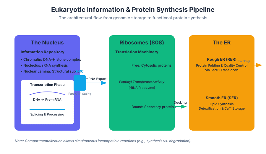
Eukaryotic cells represent a monumental leap in biological engineering. Unlike their prokaryotic counterparts, eukaryotes utilize compartmentalization—the segregation of biochemical processes into membrane-bound organelles. This spatial separation allows for the simultaneous execution of incompatible chemical reactions, such as the synthesis of proteins and their subsequent degradation, within the same cellular volume.
At its core, the eukaryotic cell is a high-throughput processing plant. It manages information (DNA), assembles components (ribosomes), performs quality control and logistics (ER and Golgi), manages waste (lysosomes), and facilitates movement (cilia and flagella). This article provides a deep-dive into the mechanics, thermodynamics, and structural biology of these critical systems.
The Nucleus: The Information Repository and Control Center
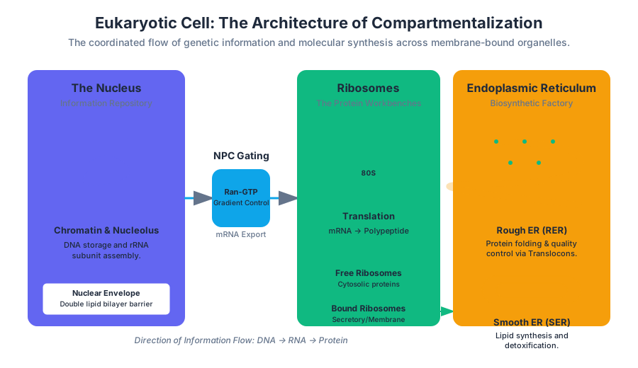
The nucleus is the defining feature of the eukaryotic cell. It serves as the central repository for the organism's genetic material and the site of transcription and RNA processing. By separating the genome from the cytoplasm, the nucleus allows for complex regulatory mechanisms, such as post-transcriptional splicing, which are unavailable to prokaryotes.
Structural Components
The nucleus is enclosed by the nuclear envelope, a double-membrane system. The outer membrane is continuous with the endoplasmic reticulum, while the inner membrane is lined by the nuclear lamina, a dense fibrillar network of intermediate filaments (lamins) that provides mechanical support.
| Component | Structure | Primary Function |
|---|---|---|
| Nuclear Envelope | Double lipid bilayer with perinuclear space | Physical barrier; regulates nucleocytoplasmic transport |
| Nuclear Pore Complex (NPC) | Octagonal protein scaffold (nucleoporins) | Selective gating of macromolecules (>40 kDa) |
| Nucleolus | Non-membrane bound sub-compartment | rRNA synthesis and ribosome subunit assembly |
| Chromatin | DNA-histone complex | Genomic packaging and epigenetic regulation |
Mechanics of Nuclear Transport
Transport across the nuclear envelope is governed by the Nuclear Pore Complex (NPC). While small molecules diffuse freely, larger proteins (>40-60 kDa) require a Nuclear Localization Signal (NLS) or a Nuclear Export Signal (NES).
The transport cycle is driven by the Ran-GTPase gradient. The concentration of Ran-GTP is high inside the nucleus (maintained by Ran-GEF) and low in the cytoplasm (maintained by Ran-GAP). This gradient provides the chemical potential necessary to drive cargo against a concentration gradient.
/*
 * Low-level simulation of Nuclear Pore Complex (NPC) gating logic.
 * This represents the selective permeability based on molecular weight
 * and the presence of a valid Nuclear Localization Signal (NLS).
 */

#include <stdio.h>
#include <stdbool.h>

#define MAX_DIFFUSION_SIZE 40.0 // kDa
#define NLS_KEY 0x5349474E // Hex representation of "SIGN"

typedef struct {
    float mass_kda;
    unsigned int signal_tag;
    char* name;
} Macromolecule;

bool check_npc_passage(Macromolecule m) {
    // Passive diffusion check
    if (m.mass_kda <= MAX_DIFFUSION_SIZE) {
        printf("[NPC] %s: Passive diffusion allowed.\n", m.name);
        return true;
    }

    // Active transport check via NLS recognition
    if (m.signal_tag == NLS_KEY) {
        printf("[NPC] %s: NLS recognized. Facilitating active transport.\n", m.name);
        return true;
    }

    printf("[NPC] %s: Access denied. Cargo too large and lacks NLS.\n", m.name);
    return false;
}

int main() {
    Macromolecule rna_pol = { 500.0, NLS_KEY, "RNA Polymerase" };
    Macromolecule glucose = { 0.18, 0, "Glucose" };
    Macromolecule stray_protein = { 120.0, 0, "Misfolded Cytoplasmic Protein" };

    check_npc_passage(rna_pol);
    check_npc_passage(glucose);
    check_npc_passage(stray_protein);

    return 0;
}
Ribosomes: The Protein Synthesis Machinery
Ribosomes are the "workbenches" of the cell, where the genetic code is translated into polypeptide chains. They are not technically organelles in the sense of being membrane-bound; rather, they are massive ribonucleoprotein (RNP) complexes.
Composition and Catalysis
A eukaryotic ribosome (80S) consists of a large subunit (60S) and a small subunit (40S). The catalytic heart of the ribosome is actually the ribosomal RNA (rRNA), making the ribosome a ribozyme. The rRNA facilitates the formation of the peptide bond through a process called peptidyl transfer.
The Central Dogma Constraint: Ribosomes can only read mRNA in the 5' to 3' direction. The rate of translation in eukaryotes is approximately 2–5 amino acids per second, significantly slower than prokaryotes (up to 20 aa/s), allowing for higher folding precision.
Free vs. Bound Ribosomes
- Free Ribosomes: Suspended in the cytosol. They synthesize proteins that function within the cytosol (e.g., glycolytic enzymes).
- Bound Ribosomes: Attached to the cytosolic side of the Endoplasmic Reticulum (ER). They synthesize proteins destined for insertion into membranes, packaging within organelles, or secretion.
The Endoplasmic Reticulum (ER): The Biosynthetic Factory
The Endoplasmic Reticulum (ER) is an extensive network of membranous tubules and sacs called cisternae. It accounts for more than half of the total membrane in many eukaryotic cells.
Rough ER (RER)
The RER is "rough" due to the presence of ribosomes on its surface. It is the primary site for the synthesis of secretory proteins. As a polypeptide is synthesized, it is threaded into the ER lumen through a protein pore called the translocon (Sec61 complex).
Smooth ER (SER)
The SER lacks ribosomes and performs diverse metabolic functions:
- Lipid Synthesis: Production of phospholipids, cholesterol, and steroid hormones.
- Detoxification: In liver cells, the SER contains enzymes (like Cytochrome P450) that add hydroxyl groups to drugs, making them more soluble and easier to flush from the body.
- Calcium Storage: In muscle cells, a specialized SER called the sarcoplasmic reticulum pumps $Ca^{2+}$ ions from the cytosol into the lumen.
Protein Folding and Quality Control
The ER lumen provides a unique oxidizing environment that favors the formation of disulfide bonds ($S-S$), which stabilize protein structures. Chaperone proteins, such as BiP, assist in folding. If a protein fails to fold correctly, it is subject to ER-Associated Degradation (ERAD), where it is exported back to the cytosol and destroyed by proteasomes.
\text{Protein Folding Success Rate } (\eta) \approx \frac{k_{fold}}{k_{fold} + k_{agg}}
Where $k_{fold}$ is the rate constant of native folding and $k_{agg}$ is the rate constant of non-specific aggregation. The ER environment is optimized to maximize $\eta$ via chaperones.
Lysosomes: The Digestive and Recycling Center
Lysosomes are membrane-bound sacs of hydrolytic enzymes used to digest macromolecules. They represent the cell's "stomach" and recycling plant.
The Acidic Microenvironment
Lysosomal enzymes (acid hydrolases) function optimally at a pH of approximately 4.5–5.0. The lysosome maintains this gradient by utilizing a V-type ATPase (proton pump) that actively transports $H^+$ ions from the cytosol (pH ~7.2) into the lysosomal lumen.
| Enzyme Category | Substrate | Resulting Product |
|---|---|---|
| Proteases | Proteins | Amino acids |
| Nucleases | Nucleic Acids | Nucleotides |
| Glycosidases | Polysaccharides | Monosaccharides |
| Lipases | Lipids | Fatty acids & Glycerol |
Mechanisms of Degradation
- Phagocytosis: Digestion of external materials (e.g., bacteria) engulfed by the cell.
- Autophagy: "Self-eating." The lysosome recycles the cell's own damaged organelles. This is a critical survival mechanism during nutrient deprivation.
Clinical Insight: Lysosomal Storage Diseases (LSDs), such as Tay-Sachs disease, occur when a specific lysosomal enzyme is missing or defective. This leads to the toxic accumulation of undigested substrates, eventually causing cellular death and organ failure.
Cilia and Flagella: Cellular Locomotion
Many eukaryotic cells possess surface appendages for movement. While they differ in length and beating patterns, cilia and flagella share a nearly identical internal ultrastructure.
The 9+2 Axoneme
The core of these structures is the axoneme, which consists of nine doublets of microtubules arranged in a ring around two central single microtubules. This is the "9+2" arrangement.
- Microtubules: Polymers of $\alpha$- and $\beta$-tubulin.
- Dynein Arms: Motor proteins attached to the outer doublets. They use ATP hydrolysis to "walk" along the adjacent microtubule.
- Nexin: Cross-linking proteins that limit the sliding of microtubules, causing the entire structure to bend instead of slide apart.
Comparison of Movement
| Feature | Cilia | Flagella |
|---|---|---|
| Length | Short (~5–10 $\mu m$) | Long (~50–200 $\mu m$) |
| Number | Numerous per cell | Usually 1 or 2 per cell |
| Motion | Oar-like (power stroke and recovery) | Undulatory (snake-like) |
| Function | Movement of cell or fluid over surface | Propulsion of the entire cell |
The Physics of the Power Stroke
The bending of a cilium is a result of the coordinated activation of dynein motors. Because the microtubules are anchored at the basal body (a structure similar to a centriole), the sliding force is converted into a bending moment.
# Simple Python model for Dynein-driven Microtubule Bending
import numpy as np

def calculate_bending_moment(force_dynein, nexin_stiffness, angle_theta):
    """
    Simplified model of the bending moment in an axoneme.
    M = F * d - k * theta
    """
    d = 24e-9  # distance between doublets in meters
    moment = (force_dynein * d) - (nexin_stiffness * angle_theta)
    return max(0, moment)

# Simulation parameters
force_per_dynein = 1.0e-12 # Newtons
active_dyneins = 500
total_force = force_per_dynein * active_dyneins
stiffness = 0.5e-18 # Nm/rad

theta_range = np.linspace(0, np.pi/4, 10)
moments = [calculate_bending_moment(total_force, stiffness, t) for t in theta_range]

for t, m in zip(theta_range, moments):
    print(f"Angle: {t:.2f} rad | Net Bending Moment: {m:.2e} Nm")
Integration: The Endomembrane System
None of these organelles operate in isolation. They are linked via the endomembrane system, a flow of membrane and proteins mediated by vesicles.
- Nucleus exports mRNA to the Cytoplasm.
- Ribosomes on the Rough ER translate mRNA into proteins.
- Proteins are folded in the ER and sent via transport vesicles to the Golgi Apparatus (not covered in detail here, but acts as the shipping center).
- The Golgi sorts proteins for delivery to the Plasma Membrane, Lysosomes, or secretion.
Common Pitfalls and Misconceptions
- "Ribosomes are organelles": While often called organelles, they are not membrane-bound. In rigorous technical contexts, they are "macromolecular machines."
- "Smooth ER only makes lipids": It is also crucial for carbohydrate metabolism (gluconeogenesis) and calcium sequestration.
- "Cilia are only for swimming": Many human cells have a primary cilium, a non-motile 9+0 structure that acts as a sensory antenna for chemical and mechanical signals.
- "The Nucleus is in the center": The position of the nucleus is highly regulated by the cytoskeleton and varies by cell type (e.g., it is pushed to the periphery in adipocytes).
Article Metadata
- Status: Peer Reviewed
- Technical Level: Level 400 (Advanced Undergraduate / Graduate)
- Domain: Molecular Cell Biology
- Last Updated: 2023.10.27
The Cell Membrane and Transport Mechanisms
Key concepts: Fluid mosaic model · Phospholipid bilayer · Passive transport · Active transport · Osmosis
How cells regulate the movement of substances in and out of their environment.
The Cell Membrane and Transport Mechanisms
The plasma membrane is not merely a static boundary; it is a sophisticated, semi-permeable interface that regulates the internal environment of the cell relative to its surroundings. This biological "operating system" manages signal transduction, molecular traffic, and structural integrity. Understanding the membrane requires a multi-disciplinary approach, blending organic chemistry, thermodynamics, and fluid mechanics.
The Phospholipid Bilayer: The Structural Foundation
At the core of every cellular membrane is the phospholipid bilayer. This structure arises spontaneously in aqueous environments due to the amphipathic nature of phospholipids—molecules containing both a polar (hydrophilic) head and non-polar (hydrophobic) tails.
Anatomy of a Phospholipid
A standard membrane phospholipid, such as phosphatidylcholine, consists of:
- A Glycerol Backbone: The central scaffold.
- Two Fatty Acid Tails: Long hydrocarbon chains (typically 14–24 carbons). One tail is usually saturated (straight), while the other is unsaturated (kinked due to a cis-double bond).
- A Phosphate Group: Linked to the third carbon of glycerol, providing a negative charge.
- An Alcohol Head Group: Attached to the phosphate (e.g., choline, serine, or ethanolamine).
The Hydrophobic Effect and Self-Assembly
The formation of the bilayer is driven by the hydrophobic effect. In water, non-polar tails disrupt the hydrogen-bonding network of water molecules, forcing them into highly ordered, energetically unfavorable "clathrate" cages. By sequestering the tails inward and exposing the polar heads to water, the system increases the entropy of the surrounding water molecules, minimizing the Gibbs free energy ($\Delta G$) of the system.
| Component | Chemical Character | Function in Membrane |
|---|---|---|
| Phosphate Head | Polar / Hydrophilic | Interfaces with intra/extracellular fluid; provides charge. |
| Saturated Tail | Non-polar / Hydrophobic | Increases packing density; reduces fluidity. |
| Unsaturated Tail | Non-polar / Hydrophobic | Introduces "kinks"; prevents tight packing; maintains fluidity. |
| Cholesterol | Steroid / Amphipathic | Temperature-dependent fluidity buffer; increases mechanical stability. |
The Thermodynamic Principle of Self-Assembly: The bilayer is a self-healing structure. If a hole is poked in the membrane, the hydrophobic tails are exposed to water, creating an energetically unstable state. The tails will spontaneously rearrange to close the gap, restoring the lowest energy state.
The Fluid Mosaic Model
Proposed by Singer and Nicolson in 1972, the Fluid Mosaic Model describes the membrane as a two-dimensional liquid where lipids and proteins diffuse laterally. It is "fluid" because the molecules are not fixed in place, and a "mosaic" because it is studded with a diverse array of proteins and carbohydrates.
Membrane Fluidity and Phase Transitions
The physical state of the membrane (liquid-disordered vs. solid-gel) is critical for protein function. This state is governed by:
- Temperature: Higher temperatures increase kinetic energy and fluidity.
- Lipid Composition: More unsaturated tails increase fluidity by preventing tight packing.
- Cholesterol: At high temperatures, cholesterol restricts lipid movement, preventing the membrane from becoming too "leaky." At low temperatures, it prevents tails from crystallizing, maintaining fluidity.
Membrane Proteins
Proteins account for approximately 50% of the membrane's mass. They are categorized by their relationship to the bilayer:
- Integral Proteins: Span the entire bilayer (transmembrane). They typically feature alpha-helical domains composed of hydrophobic amino acids (e.g., Leucine, Valine) that interface with the lipid tails.
- Peripheral Proteins: Attached to the membrane surface or to integral proteins via non-covalent bonds.
- Lipid-Anchored Proteins: Covalently bonded to lipid molecules embedded in the bilayer.
Implementation: Simulating Lipid Interaction
In computational biology, we often model the interaction between lipids using a Lennard-Jones potential to simulate the van der Waals forces that keep the bilayer together.
/*
 * A simplified Lennard-Jones potential calculation for
 * molecular dynamics simulation of lipid tail interactions.
 */
#include <math.h>
#include <stdio.h>

typedef struct {
    double x, y, z;
} Vector3;

double calculate_lj_potential(Vector3 p1, Vector3 p2, double epsilon, double sigma) {
    double dx = p1.x - p2.x;
    double dy = p1.y - p2.y;
    double dz = p1.z - p2.z;
    double r2 = dx*dx + dy*dy + dz*dz;
    double r6 = pow(sigma * sigma / r2, 3);
    double r12 = r6 * r6;

    // V(r) = 4 * epsilon * [(sigma/r)^12 - (sigma/r)^6]
    return 4.0 * epsilon * (r12 - r6);
}

int main() {
    Vector3 lipid_a = {0.0, 0.0, 0.0};
    Vector3 lipid_b = {0.0, 0.0, 3.8}; // Distance in Angstroms
    double energy = calculate_lj_potential(lipid_a, lipid_b, 0.2, 3.4);
    printf("Inter-lipid Potential Energy: %f kcal/mol\n", energy);
    return 0;
}
Passive Transport: Diffusion and Facilitated Transport
Passive transport is the movement of solutes across the membrane without the expenditure of metabolic energy (ATP). This process is driven by the increase in entropy as solutes move from an area of high concentration to an area of low concentration.
Simple Diffusion
Small, non-polar molecules (e.g., $O_2$, $CO_2$, $N_2$) and small uncharged polar molecules (e.g., ethanol) can pass directly through the lipid bilayer. The rate of diffusion is governed by Fick’s First Law.
Mathematical Derivation: Fick's First Law
The flux ($J$) of a substance across a membrane is proportional to the concentration gradient ($\frac{dC}{dx}$):
J = -D \frac{dC}{dx}
Where:
- $J$ is the diffusion flux (amount of substance per unit area per unit time).
- $D$ is the diffusion coefficient (determined by the solute's size and the membrane's viscosity).
- $\frac{dC}{dx}$ is the concentration gradient.
For a membrane of thickness $\Delta x$, the equation simplifies to: $J = P(C_{out} - C_{in})$, where $P$ is the permeability coefficient.
Facilitated Diffusion
Large or charged molecules (e.g., glucose, ions like $Na^+$) cannot cross the hydrophobic core. They require specialized proteins:
- Channel Proteins: Form hydrophilic pores (e.g., Aquaporins for water, Ion channels).
- Carrier Proteins: Bind the solute and undergo a conformational change to transfer it to the other side (e.g., GLUT1 glucose transporter).
| Feature | Simple Diffusion | Facilitated Diffusion |
|---|---|---|
| Energy Required | No | No |
| Protein Required | No | Yes (Channel or Carrier) |
| Specificity | Low | High |
| Saturation Kinetics | No (Linear) | Yes (Vmax limited) |
| Examples | $O_2$, Steroids | Glucose, $K^+$ |
Osmosis and Tonicity
Osmosis is the specific case of passive transport involving the movement of water across a semi-permeable membrane. Water moves from a region of low solute concentration (high water potential) to a region of high solute concentration (low water potential).
The van 't Hoff Equation for Osmotic Pressure
Osmotic pressure ($\Pi$) is the pressure required to stop the flow of water. It is calculated as:
\Pi = iMRT
Where:
- $i$ = van 't Hoff factor (number of particles the solute dissociates into, e.g., $NaCl = 2$).
- $M$ = Molarity (mol/L).
- $R$ = Ideal gas constant ($0.0821 \ L \cdot atm / mol \cdot K$).
- $T$ = Absolute temperature (Kelvin).
Tonicity and Cell Morphology
Tonicity describes how an extracellular solution affects cell volume. It is a relative measure.
| Solution Type | Solute Concentration | Water Movement | Effect on Animal Cell | Effect on Plant Cell |
|---|---|---|---|---|
| Isotonic | Equal to cytosol | No net movement | Normal (Flaccid) | Flaccid |
| Hypotonic | Lower than cytosol | Into the cell | Lysis (Bursting) | Turgid (Normal) |
| Hypertonic | Higher than cytosol | Out of the cell | Crenation (Shriveling) | Plasmolysis |
Common Pitfall: Students often confuse "osmolarity" with "tonicity." Osmolarity is an absolute measure of solute concentration ($Osm/L$), while tonicity is a functional measure of how a solution affects a specific cell, which depends on both osmolarity and the permeability of the membrane to those solutes.
Active Transport: Moving Against the Gradient
Active transport requires energy to move solutes against their electrochemical gradient. This is essential for maintaining internal concentrations of ions that differ significantly from the environment.
Primary Active Transport
Energy is derived directly from the hydrolysis of ATP. The most critical example is the Sodium-Potassium Pump ($Na^+/K^+$ ATPase).
- Three $Na^+$ ions bind to the pump from the cytosol.
- ATP phosphorylates the pump, causing a conformational change.
- $Na^+$ is released to the extracellular fluid.
- Two $K^+$ ions bind from the outside.
- The phosphate group is released, returning the pump to its original shape.
- $K^+$ is released into the cytosol.
This pump maintains a high $[K^+]$ and low $[Na^+]$ inside the cell, creating an electrochemical gradient used for signaling and secondary transport.
Secondary Active Transport (Cotransport)
This mechanism uses the potential energy stored in an electrochemical gradient (created by primary transport) to move another substance.
- Symport: Both substances move in the same direction (e.g., SGLT1 moves Glucose into the cell using the $Na^+$ gradient).
- Antiport: Substances move in opposite directions (e.g., $Na^+/Ca^{2+}$ exchanger).
Implementation: Modeling the Nernst Equation
The equilibrium potential of an ion (where the chemical gradient is balanced by the electrical gradient) is defined by the Nernst Equation.
import numpy as np

def calculate_nernst_potential(z, temp_c, c_out, c_in):
    """
    Calculates the equilibrium potential (E_ion) in millivolts.
    z: Valence of the ion (e.g., +1 for Na+, -1 for Cl-)
    temp_c: Temperature in Celsius
    c_out: Extracellular concentration (mM)
    c_in: Intracellular concentration (mM)
    """
    R = 8.314  # Gas constant
    F = 96485  # Faraday constant
    T = temp_c + 273.15 # Convert to Kelvin

    # E = (RT / zF) * ln(C_out / C_in)
    # Factor for mV conversion and log10: 61.5 at 37C
    potential = (R * T / (z * F)) * np.log(c_out / c_in)
    return potential * 1000 # Convert to mV

# Example: Potassium (K+) at body temperature
# Typical: K_out = 5mM, K_in = 140mM
e_k = calculate_nernst_potential(1, 37, 5, 140)
print(f"Equilibrium Potential for K+: {e_k:.2f} mV")
Bulk Transport: Endocytosis and Exocytosis
When the cell needs to transport large particles (proteins, bacteria, or large volumes of fluid), it uses bulk transport, which involves the folding and fusing of the membrane itself.
Endocytosis
The cell takes in materials by forming new vesicles from the plasma membrane.
- Phagocytosis ("Cell eating"): The cell engulfs large particles or whole cells.
- Pinocytosis ("Cell drinking"): The cell gulps droplets of extracellular fluid into tiny vesicles.
- Receptor-Mediated Endocytosis: Highly specific; triggered when ligands bind to receptors (e.g., Cholesterol uptake via LDL receptors).
Exocytosis
Vesicles from the cell's interior fuse with the plasma membrane, releasing their contents to the outside. This is the primary method for secreting hormones, neurotransmitters, and digestive enzymes.
Summary of Transport Mechanisms
| Mechanism | Direction | Energy Source | Protein Involved | Specificity |
|---|---|---|---|---|
| Simple Diffusion | Down gradient | Kinetic energy | None | Low |
| Facilitated Diffusion | Down gradient | Kinetic energy | Channel/Carrier | High |
| Osmosis | Toward high solute | Kinetic energy | Aquaporins | High |
| Primary Active | Against gradient | ATP Hydrolysis | Pump (ATPase) | High |
| Secondary Active | Against gradient | Ion gradient | Cotransporter | High |
| Bulk Transport | Varies | ATP | Cytoskeleton/Vesicle | Varies |

Metabolism and Enzymatic Activity
Key concepts: Anabolism vs. Catabolism · Enzymes · Activation Energy (Ea) · Gluconeogenesis
The chemical reactions that sustain life and the biological catalysts that speed them up.
Metabolism and Enzymatic Activity
Metabolism is the totality of an organism's chemical reactions, a highly coordinated and purposeful activity in which multi-enzyme systems (metabolic pathways) cooperate to satisfy the energetic and structural needs of the cell. At its core, metabolism is a matter of energy management: the conversion of energy from the environment into biologically useful forms, and the synthesis of the molecular building blocks of life.
The Thermodynamic Framework of Metabolism
To understand metabolism, one must first understand the governing laws of thermodynamics. The directionality of metabolic reactions is determined by the change in Gibbs Free Energy ($\Delta G$).
The Gibbs Free Energy Equation: $$\Delta G = \Delta H - T\Delta S$$ Where $\Delta H$ is the change in enthalpy (heat content), $T$ is the absolute temperature in Kelvin, and $\Delta S$ is the change in entropy (disorder).
A reaction is spontaneous (exergonic) only if $\Delta G$ is negative. However, many essential biological processes are endergonic ($\Delta G > 0$). Life persists by coupling these unfavorable reactions to highly favorable ones, typically the hydrolysis of Adenosine Triphosphate (ATP).
Anabolism vs. Catabolism: The Metabolic Seesaw
Metabolism is bifurcated into two broad, opposing, yet complementary phases: Catabolism and Anabolism. These pathways are rarely simple linear chains; they are complex networks of interconnected nodes.
Catabolism: The Degradative Phase
Catabolism involves the breakdown of complex organic molecules (carbohydrates, lipids, proteins) into simpler end products (e.g., $CO_2$, $NH_3$, $H_2O$). This process is oxidative and releases free energy, some of which is captured in the form of ATP and reduced electron carriers (NADH, $FADH_2$).
Anabolism: The Biosynthetic Phase
Anabolism, or biosynthesis, is the synthesis of complex molecules from simpler precursors. These processes are reductive and require an input of energy, typically fueled by the ATP generated during catabolism.
| Feature | Catabolism | Anabolism |
|---|---|---|
| Primary Goal | Energy production (ATP generation) | Biosynthesis of macromolecules |
| Thermodynamics | Exergonic ($\Delta G < 0$) | Endergonic ($\Delta G > 0$) |
| Redox State | Oxidative (loss of electrons) | Reductive (gain of electrons) |
| Common Carriers | $NAD^+ \rightarrow NADH$ | $NADPH \rightarrow NADP^+$ |
| Molecular Complexity | Complex $\rightarrow$ Simple | Simple $\rightarrow$ Complex |
| Example | Glycolysis, Citric Acid Cycle | Gluconeogenesis, Protein Synthesis |
Enzymes: The Biological Catalysts
If metabolism is the "what" of cellular life, enzymes are the "how." Most biological reactions, while thermodynamically favorable, occur at rates far too slow to sustain life. Enzymes are typically proteins (though some are RNA-based ribozymes) that accelerate reaction rates by factors of $10^6$ to $10^{12}$.
The Mechanism of Catalysis
Enzymes do not alter the equilibrium of a reaction ($\Delta G$ remains unchanged); instead, they lower the Activation Energy ($E_a$). They achieve this by stabilizing the transition state, a high-energy, transient molecular configuration that must be reached for the reaction to proceed.
- Substrate Binding: The substrate binds to the enzyme's active site via weak interactions (hydrogen bonds, ionic bonds, van der Waals forces).
- Induced Fit: The enzyme undergoes a conformational change to wrap more tightly around the substrate, orienting it for the reaction.
- Catalysis: The enzyme provides a microenvironment (e.g., acidic/basic residues, metal ions) that lowers the energy barrier.
- Product Release: The products have a lower affinity for the active site and are released, leaving the enzyme unchanged and ready for another cycle.
Enzyme Kinetics: The Michaelis-Menten Model
The relationship between substrate concentration $[S]$ and reaction velocity $v$ is described by the Michaelis-Menten equation.
v = \frac{V_{max} [S]}{K_m + [S]}
Where:
- $V_{max}$: The maximum velocity of the reaction when the enzyme is saturated with substrate.
- $K_m$ (Michaelis Constant): The substrate concentration at which the velocity is half of $V_{max}$. It is an inverse measure of the enzyme's affinity for its substrate.
Implementation: Simulating Enzyme Kinetics
In computational biology, we often model these kinetics to predict how a system will respond to changes in substrate availability or inhibitor presence.
import numpy as np
import matplotlib.pyplot as plt

def michaelis_menten(S, Vmax, Km):
    """
    Calculates reaction velocity based on Michaelis-Menten kinetics.
    """
    return (Vmax * S) / (Km + S)

# Parameters for a hypothetical enzyme (e.g., Hexokinase)
VMAX = 100.0  # micromoles/min
KM = 5.0      # millimolar

# Substrate concentrations from 0 to 50 mM
substrate_concentrations = np.linspace(0, 50, 500)
velocities = michaelis_menten(substrate_concentrations, VMAX, KM)

# Plotting the saturation curve
plt.figure(figsize=(10, 6))
plt.plot(substrate_concentrations, velocities, label=f'Vmax={VMAX}, Km={KM}')
plt.axhline(y=VMAX, color='r', linestyle='--', label='Vmax')
plt.axhline(y=VMAX/2, color='g', linestyle='--', label='1/2 Vmax')
plt.axvline(x=KM, color='b', linestyle=':', label='Km')
plt.title('Enzyme Saturation Curve')
plt.xlabel('Substrate Concentration [S] (mM)')
plt.ylabel('Reaction Velocity (v)')
plt.legend()
plt.grid(True)
plt.show()
Activation Energy ($E_a$) and the Transition State
The Activation Energy ($E_a$) is the "hump" on a reaction coordinate diagram. It represents the kinetic barrier that prevents all exergonic reactions from happening instantaneously.
The Arrhenius Equation
The rate constant $k$ of a reaction is exponentially dependent on the activation energy:
k = A e^{-\frac{E_a}{RT}}
Where:
- $A$ is the frequency factor.
- $R$ is the gas constant ($8.314 , J/mol \cdot K$).
- $T$ is the temperature.
Small decreases in $E_a$ result in massive increases in the rate constant $k$. Enzymes lower $E_a$ through several strategies:
- Proximity and Orientation: Bringing reactants together in the correct geometry.
- Desolvation: Removing the water shell around the substrate to facilitate interaction.
- Acid-Base Catalysis: Using amino acid side chains to donate or accept protons.
- Covalent Catalysis: Forming a transient covalent bond between the enzyme and substrate.
| Strategy | Description | Example |
|---|---|---|
| Acid-Base | Proton transfer to stabilize charges | Chymotrypsin (Histidine residue) |
| Covalent | Formation of a transient enzyme-substrate bond | Glyceraldehyde 3-phosphate dehydrogenase |
| Metal Ion | Use of $Mg^{2+}$, $Zn^{2+}$, etc., to orient substrates | DNA Polymerase ($Mg^{2+}$) |
| Electrostatic | Charge-charge interactions in the active site | Superoxide dismutase |
Gluconeogenesis: A Case Study in Anabolism
Gluconeogenesis is the metabolic pathway through which organisms synthesize glucose from non-carbohydrate precursors (e.g., pyruvate, lactate, glycerol, and glucogenic amino acids). This process is vital during fasting or intense exercise to maintain blood glucose levels for the brain and red blood cells.
Why it isn't just "Reverse Glycolysis"
While gluconeogenesis shares seven enzymes with glycolysis, it is not a simple reversal. Glycolysis has three "irreversible" steps with highly negative $\Delta G$:
- Glucose $\rightarrow$ Glucose-6-Phosphate (Hexokinase)
- Fructose-6-Phosphate $\rightarrow$ Fructose-1,6-Bisphosphate (PFK-1)
- Phosphoenolpyruvate (PEP) $\rightarrow$ Pyruvate (Pyruvate Kinase)
Gluconeogenesis must bypass these steps using different enzymes to ensure the overall pathway is thermodynamically favorable ($\Delta G \approx -38 , kJ/mol$).
The Bypasses of Gluconeogenesis
- Pyruvate to PEP: This requires two steps. Pyruvate is first converted to oxaloacetate by Pyruvate Carboxylase (requiring ATP and Biotin), and then oxaloacetate is converted to PEP by PEP Carboxykinase (requiring GTP).
- Fructose-1,6-Bisphosphate to Fructose-6-Phosphate: Catalyzed by Fructose-1,6-bisphosphatase. This is the key regulatory step.
- Glucose-6-Phosphate to Glucose: Catalyzed by Glucose-6-phosphatase, found primarily in the liver and kidneys.
The Cost of Gluconeogenesis: Synthesis of 1 mole of glucose from 2 moles of pyruvate requires:
2 Pyruvate + 4 ATP + 2 GTP + 2 NADH + 2 H+ + 6 H2O → Glucose + 4 ADP + 2 GDP + 6 Pi + 2 NAD+It is an energetically expensive process, consuming 6 high-energy phosphate bonds.
Derivation: The Energetic Barrier of Pyruvate Kinase
To see why a bypass is needed, consider the $\Delta G$ of the Pyruvate Kinase reaction in glycolysis: $PEP + ADP \rightarrow Pyruvate + ATP \quad (\Delta G'^\circ = -31.4 , kJ/mol)$ The reverse reaction ($Pyruvate + ATP \rightarrow PEP + ADP$) would have a $\Delta G'^\circ$ of $+31.4 , kJ/mol$, making it virtually impossible under cellular conditions without the two-step bypass involving oxaloacetate.
DERIVATION OF THE BYPASS THERMODYNAMICS:
Step 1: Pyruvate + HCO3- + ATP -> Oxaloacetate + ADP + Pi  (dG1)
Step 2: Oxaloacetate + GTP -> PEP + CO2 + GDP             (dG2)
---------------------------------------------------------------
Net: Pyruvate + ATP + GTP -> PEP + ADP + GDP + Pi         (dG_net)

By splitting the reaction, the cell uses two high-energy
phosphoryl group transfers (ATP and GTP) to push the
equilibrium toward PEP synthesis.
Regulation of Metabolic Flux
Metabolic pathways are regulated to prevent futile cycles (e.g., glycolysis and gluconeogenesis running simultaneously at high rates).
Allosteric Regulation
Enzymes like Phosphofructokinase-1 (PFK-1) in glycolysis and Fructose-1,6-bisphosphatase (FBPase-1) in gluconeogenesis are reciprocally regulated by the same molecules.
- AMP: Signals low energy. It activates PFK-1 and inhibits FBPase-1.
- Citrate: Signals high energy/biosynthetic precursors. It inhibits PFK-1 and activates FBPase-1.
- Fructose-2,6-bisphosphate: The most potent allosteric effector, which stimulates glycolysis and inhibits gluconeogenesis.
Data Representation: Metabolic Intermediates
In a laboratory or clinical database, metabolic states are often tracked via concentrations of these intermediates.
-- Schema for tracking metabolic flux in a simulated liver cell
CREATE TABLE metabolic_intermediates (
    intermediate_id INT PRIMARY KEY,
    name VARCHAR(50),
    concentration_micromolar FLOAT,
    pathway_association ENUM('Glycolysis', 'Gluconeogenesis', 'Both'),
    last_updated TIMESTAMP
);

INSERT INTO metabolic_intermediates (name, concentration_micromolar, pathway_association)
VALUES
('Glucose-6-Phosphate', 120.5, 'Both'),
('Fructose-1,6-Bisphosphate', 25.2, 'Both'),
('Phosphoenolpyruvate', 15.8, 'Both'),
('Pyruvate', 80.0, 'Both'),
('Oxaloacetate', 0.5, 'Gluconeogenesis');

-- Query to identify potential bottlenecks in Gluconeogenesis
SELECT name, concentration_micromolar
FROM metabolic_intermediates
WHERE pathway_association IN ('Gluconeogenesis', 'Both')
ORDER BY concentration_micromolar ASC;
Common Pitfalls and Misconceptions
- Misconception: Enzymes change the $\Delta G$ of a reaction.
- Correction: Enzymes only change the rate ($k$), not the thermodynamic favorability or the equilibrium constant ($K_{eq}$).
- Misconception: Anabolism and Catabolism are just the reverse of each other.
- Correction: They often use different enzymes for key steps and occur in different cellular compartments (e.g., fatty acid synthesis in the cytosol vs. breakdown in the mitochondria) to allow for independent regulation.
- Misconception: Gluconeogenesis happens in all cells.
- Correction: It is primarily a hepatic (liver) and renal (kidney) process. Muscle cells lack Glucose-6-phosphatase and therefore cannot release glucose into the blood.
Summary of Metabolic Integration
Metabolism is a dynamic equilibrium. The cell constantly monitors its energy charge ($[ATP]/[AMP]$ ratio) and adjusts the flux through catabolic and anabolic pathways. Enzymes serve as the logic gates in this biological circuit, integrating chemical signals to maintain homeostasis.
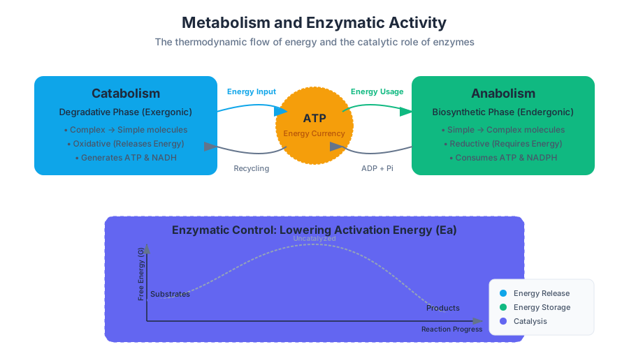
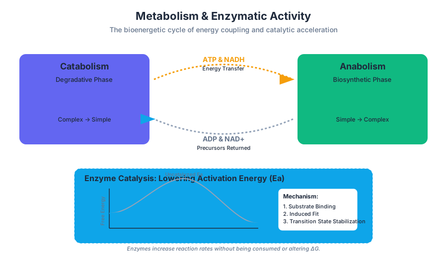
Cellular Energy: Photosynthesis and Respiration
Key concepts: Photosynthesis · Cellular Respiration · ATP · Energy transformation
How organisms transform energy from the sun or food into a usable form (ATP).
Cellular Energy: Photosynthesis and Respiration
In the biological theater, energy is the fundamental currency that dictates the feasibility of every cellular transaction. From the synthesis of complex macromolecules to the mechanical contraction of muscle fibers, life operates under the strict constraints of thermodynamics. This article explores the dual engines of life: Photosynthesis, which captures and stores solar energy in chemical bonds, and Cellular Respiration, which harvests that energy to produce Adenosine Triphosphate (ATP).
The Thermodynamic Foundation of Metabolism
Metabolism is the sum of all chemical reactions within an organism. These reactions are categorized into two broad pathways that maintain the cell's internal order against the tide of entropy.
- Anabolism: The "building up" phase. These are endergonic reactions, meaning they require an input of energy ($\Delta G > 0$) to synthesize complex molecules from simpler precursors (e.g., building a protein from amino acids).
- Catabolism: The "breaking down" phase. These are exergonic reactions, releasing stored energy ($\Delta G < 0$) by degrading complex molecules into simpler ones (e.g., the breakdown of glucose).
The First Law of Thermodynamics in Biology: Energy cannot be created or destroyed, only transformed. In cells, light energy is transformed into chemical bond energy, which is then transformed into work and heat.
Energy Coupling and ATP
Cells perform work by energy coupling, using an exergonic process to drive an endergonic one. The mediator of this coupling is ATP. Structurally, ATP consists of an adenine nitrogenous base, a ribose sugar, and three phosphate groups. The bonds between the phosphate groups are often called "high-energy bonds," but more accurately, they are unstable bonds due to the mutual repulsion of the negatively charged phosphate groups.
| Parameter | ATP (Adenosine Triphosphate) | ADP (Adenosine Diphosphate) |
|---|---|---|
| Phosphate Groups | 3 | 2 |
| Energy State | High (Potential Energy) | Low |
| Role | Energy Donor | Energy Acceptor |
| Stability | Relatively Unstable | More Stable |
| Hydrolysis $\Delta G$ | $\approx -30.5$ kJ/mol | N/A |
Photosynthesis: Harvesting the Light
Photosynthesis is the primary anabolic pathway of the biosphere. It occurs in the chloroplasts of plants and algae, and in the plasma membranes of certain prokaryotes. The process is summarized by the equation:
6CO_2 + 6H_2O + \text{Light Energy} \rightarrow C_6H_{12}O_6 + 6O_2
The Light-Dependent Reactions
These reactions occur in the thylakoid membranes. They convert solar energy into the chemical energy of ATP and NADPH.
- Photoexcitation: Chlorophyll molecules absorb photons, boosting electrons to a higher energy state.
- Photosystem II (PSII): Water is split (photolysis), releasing $O_2$, protons ($H^+$), and electrons. These electrons replace those lost by chlorophyll.
- Electron Transport Chain (ETC): Electrons move through a series of proteins, pumping $H^+$ into the thylakoid space, creating a proton gradient.
- Photosystem I (PSI): Electrons are re-energized by light and used to reduce $NADP^+$ to $NADPH$.
- Chemiosmosis: The $H^+$ gradient drives ATP Synthase to produce ATP from ADP and inorganic phosphate ($P_i$).
The Light-Independent Reactions (Calvin Cycle)
Occurring in the stroma, this cycle uses the ATP and NADPH from the light reactions to "fix" carbon from $CO_2$ into sugar.
- Phase 1: Carbon Fixation: The enzyme RuBisCO attaches $CO_2$ to a five-carbon sugar, Ribulose Bisphosphate (RuBP).
- Phase 2: Reduction: The resulting molecules are phosphorylated by ATP and reduced by NADPH to form Glyceraldehyde-3-phosphate (G3P).
- Phase 3: Regeneration: Some G3P molecules exit to form glucose, while others are recycled to regenerate RuBP.
Cellular Respiration: The Engine of Catabolism
Cellular respiration is the process by which cells extract energy from food molecules. While it can occur anaerobically (fermentation), aerobic respiration is the most efficient, utilizing oxygen as the final electron acceptor.
Stage 1: Glycolysis
Glycolysis occurs in the cytosol and does not require oxygen. It breaks down one molecule of glucose ($C_6$) into two molecules of pyruvate ($C_3$).
- Energy Investment: 2 ATP are consumed to phosphorylate glucose.
- Energy Payoff: 4 ATP and 2 NADH are produced.
- Net Yield: 2 ATP, 2 NADH, and 2 Pyruvate.
Stage 2: The Citric Acid Cycle (Krebs Cycle)
Before entering the cycle, pyruvate is converted into Acetyl-CoA in the mitochondrial matrix, releasing $CO_2$ and producing NADH. The Krebs Cycle then fully oxidizes the acetyl group.
| Input (per Glucose) | Output (per Glucose) |
|---|---|
| 2 Acetyl-CoA | 4 $CO_2$ |
| 6 $NAD^+$ | 6 $NADH$ |
| 2 $FAD$ | 2 $FADH_2$ |
| 2 $ADP + P_i$ | 2 $ATP$ (via GTP) |
Stage 3: Oxidative Phosphorylation
This is the "grand finale" occurring on the inner mitochondrial membrane (cristae). It consists of the Electron Transport Chain and Chemiosmosis.
- Electron Transport: NADH and $FADH_2$ donate electrons to the ETC. As electrons move down the chain toward Oxygen (the final acceptor), energy is used to pump $H^+$ into the intermembrane space.
- Proton-Motive Force: The resulting electrochemical gradient represents stored potential energy.
- ATP Synthesis: $H^+$ ions flow back into the matrix through ATP Synthase, which acts like a molecular turbine, spinning to catalyze the synthesis of ATP.
Technical Implementation: Modeling Metabolic Flux
In computational biology, we often model these reactions using Flux Balance Analysis (FBA). Below is a Python implementation using a simplified stoichiometric matrix to calculate the theoretical yield of a metabolic pathway.
import numpy as np

def calculate_metabolic_yield(stoichiometry_matrix, reaction_rates):
    """
    Calculates the net production of metabolites given a
    stoichiometric matrix (S) and a vector of reaction rates (v).
    S * v = dX/dt (Rate of change of metabolite concentrations)
    """
    # S matrix: Rows are metabolites, Columns are reactions
    # Negative values are reactants, positive are products

    # Example: [Glucose, ATP, NADH, Pyruvate]
    # Reaction 1 (Glycolysis): -1 Glucose + 2 ATP + 2 NADH + 2 Pyruvate

    net_change = np.dot(stoichiometry_matrix, reaction_rates)
    return net_change

# Stoichiometric Matrix for a simplified Glycolysis + TCA model
# Rows: [Glucose, Pyruvate, CO2, ATP, NADH]
S = np.array([
    [-1,  0,  0], # Glucose
    [ 2, -1,  0], # Pyruvate
    [ 0,  3,  0], # CO2
    [ 2,  1, 32], # ATP (Glycolysis, TCA, ETC/OxPhos)
    [ 2,  4, -10] # NADH (Produced in Glyc/TCA, consumed in ETC)
])

# Reaction rates (v): [v_glycolysis, v_tca, v_oxphos]
v = np.array([1, 2, 0.6]) # Arbitrary flux units

yields = calculate_metabolic_yield(S, v)
metabolites = ["Glucose", "Pyruvate", "CO2", "ATP", "NADH"]

print("Metabolic Flux Results:")
for met, val in zip(metabolites, yields):
    print(f"{met:10}: {val:>6.2f}")
The Efficiency of Energy Transformation
How efficient is the cell at converting the energy in glucose into ATP? We can derive this using the standard Gibbs free energy change.
\text{Efficiency} = \frac{\text{Energy captured in ATP}}{\text{Total energy available in Glucose}} \times 100
Mathematical Derivation of Efficiency
- Energy in Glucose: The complete oxidation of one mole of glucose releases $\Delta G = -686$ kcal/mol.
- Energy in ATP: The phosphorylation of ADP to ATP requires $\Delta G = +7.3$ kcal/mol.
- Total ATP Yield: Under ideal conditions, one molecule of glucose yields approximately 30 to 32 ATP.
Let's calculate the efficiency for 32 ATP:
Energy Captured = 32 moles ATP * 7.3 kcal/mol = 233.6 kcal
Efficiency = (233.6 / 686) * 100
Efficiency ≈ 34%
The remaining 66% of the energy is released as heat, which is not "wasted" in endothermic organisms but used to maintain body temperature.
Gluconeogenesis: The Anabolic Mirror
When glucose levels are low, the body performs Gluconeogenesis—the synthesis of glucose from non-carbohydrate precursors (like lactate, glycerol, or certain amino acids). While it shares many enzymes with glycolysis, it is not a simple reversal.
Le Chatelier’s Principle and Irreversibility: Three steps in glycolysis are highly exergonic and essentially irreversible ($\Delta G \ll 0$). Gluconeogenesis bypasses these steps using different enzymes to ensure the pathway is thermodynamically favorable in the direction of glucose synthesis.
Key Bypass Reactions
| Glycolysis Enzyme | Gluconeogenesis Bypass Enzyme | Significance |
|---|---|---|
| Hexokinase | Glucose-6-phosphatase | Allows glucose to exit the cell |
| Phosphofructokinase (PFK) | Fructose-1,6-bisphosphatase | Major regulatory point |
| Pyruvate Kinase | Pyruvate Carboxylase & PEP Carboxykinase | Requires ATP and GTP input |
Real-World Application: Bioinformatics and Mitochondrial Analysis
In clinical settings, analyzing the efficiency of cellular respiration often involves looking at mitochondrial DNA (mtDNA) or the expression of ETC proteins. Researchers use tools like blast to compare mitochondrial genomes across species or identify mutations that lead to metabolic disorders.
# Example: Using NCBI BLAST+ to compare a human mitochondrial
# protein (Cytochrome c oxidase) against a database.

# 1. Create a blast database from a local protein file
makeblastdb -in mitochondrial_proteome.fasta -dbtype prot -out mito_db

# 2. Run BLASTP to find homologs of a specific respiratory enzyme
blastp -query human_cox1.fasta -db mito_db -out results.txt \
       -evalue 1e-5 -outfmt "6 qseqid sseqid pident evalue"

# 3. Filter results for high identity (>90%) indicating conserved function
awk '$3 > 90' results.txt
Common Pitfalls and Misconceptions
- "Plants only do photosynthesis": This is a major error. Plants have mitochondria and perform cellular respiration 24/7 to power cellular work. Photosynthesis only provides the fuel.
- "The purpose of the ETC is to make ATP": Strictly speaking, the ETC's purpose is to create a proton gradient. ATP Synthase is the enzyme that actually synthesizes ATP. If the membrane is "leaky" (uncoupled), the ETC will run, but no ATP will be made (energy is lost as heat).
- "High energy bonds": As mentioned, the energy isn't "in" the bond itself like a battery. The energy release comes from the fact that the products (ADP + $P_i$) are significantly more stable and have lower free energy than the reactant (ATP).
Summary of Interconnectivity
The relationship between photosynthesis and respiration is a perfect cycle of matter. The oxygen produced in the thylakoid becomes the terminal electron acceptor in the mitochondria. The $CO_2$ produced in the Krebs cycle becomes the substrate for RuBisCO in the Calvin cycle.
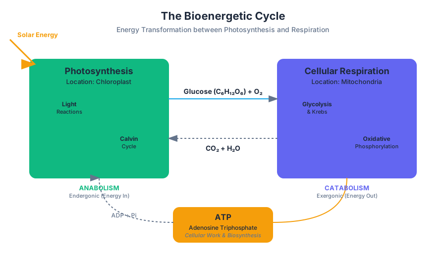
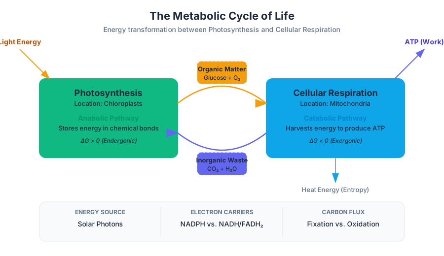
Cellular Reproduction: Mitosis and Meiosis
Key concepts: The Cell Cycle · Mitosis · Meiosis · Chromatids and Chromatin · Crossover
The mechanics of cell division for growth, repair, and the production of gametes.
Cellular Reproduction: Mitosis and Meiosis
Cellular reproduction is the fundamental process by which life propagates, grows, and maintains its structural integrity. At its core, it is an information-theory problem: how does a biological system replicate a massive, complex instruction set (the genome) and distribute it with high fidelity to progeny? In multicellular organisms, this process bifurcates into two distinct pathways: Mitosis, the mechanism of somatic growth and asexual replication, and Meiosis, the specialized division required for sexual reproduction and genetic diversification.
The Physical Substrate: Chromatin, Chromatids, and Chromosomes
Before analyzing the mechanics of division, we must define the state of the genetic material. DNA does not exist as a loose "soup" within the nucleus; it is highly organized through a hierarchy of protein-DNA complexes.
Definitions and Hierarchy
The terminology of DNA packaging is often a source of confusion. The distinction lies in the level of condensation and the replication state:
- Chromatin: The "working state" of DNA. It consists of DNA wrapped around histone proteins (nucleosomes). During Interphase, chromatin is relatively decondensed to allow transcription factors and polymerases access to the genetic code.
- Chromatid: Following the S phase of the cell cycle, each chromosome is replicated. The two identical copies are called sister chromatids. They are joined at a specialized DNA sequence called the centromere.
- Chromosome: A single, continuous molecule of DNA. In its unreplicated state, one chromosome equals one chromatid. In its replicated state (post-S phase), one chromosome consists of two sister chromatids.
| Feature | Chromatin | Chromatid | Chromosome |
|---|---|---|---|
| Structure | "Beads on a string" (nucleosomes) | One half of a replicated chromosome | The complete physical unit of heredity |
| Visibility | Visible only with electron microscopy | Visible during Mitosis/Meiosis | Highly condensed during M-phase |
| Function | Gene expression and DNA packaging | Ensuring equal distribution of DNA | Large-scale genomic organization |
| Composition | DNA + Histones | DNA + Histones + Cohesin proteins | DNA + Histones + Scaffolding proteins |
The Centromere Theorem: The number of chromosomes in a cell is always equal to the number of functional centromeres, regardless of how many chromatids are attached to them.
The Cell Cycle: The Orchestration of Division
The Cell Cycle is the ordered sequence of events that a cell undergoes from its "birth" to its own division. It is governed by a complex regulatory network of Cyclins and Cyclin-Dependent Kinases (CDKs) that act as logic gates, ensuring that one stage is completed before the next begins.
Phases of the Cycle
The cycle is divided into two primary epochs: Interphase (preparation) and the M-phase (division).
- G1 Phase (Gap 1): The cell grows and performs normal metabolic functions. It monitors the environment for growth factors and DNA integrity.
- S Phase (Synthesis): DNA replication occurs. The DNA content doubles ($2n \to 4n$ in terms of mass, though the chromosome count remains $2n$).
- G2 Phase (Gap 2): Further growth and protein synthesis. The cell checks for replication errors.
- M Phase (Mitotic Phase): The physical separation of the nucleus (Mitosis) and the cytoplasm (Cytokinesis).
Checkpoint Logic
The cell cycle is not a simple timer; it is a state machine with conditional transitions.
| Checkpoint | Timing | Criteria for Success | Failure Consequence |
|---|---|---|---|
| G1 Checkpoint | Late G1 | Sufficient nutrients, growth factors, no DNA damage | Entry into G0 (quiescence) or Apoptosis |
| G2 Checkpoint | End of G2 | DNA replication complete, no damage | Cell cycle arrest for DNA repair |
| Spindle Checkpoint | Metaphase | All chromosomes attached to spindle fibers | Delay of Anaphase (prevents aneuploidy) |
Mitosis: The Algorithm of Identity
Mitosis is the process of equational division. Its goal is to produce two daughter cells that are genetically identical to the parent cell. This is the mechanism used for embryonic development, tissue renewal, and wound healing.
The Mechanics of Mitosis
Mitosis is traditionally divided into five stages:
- Prophase: Chromatin condenses into visible chromosomes. The nucleolus disappears, and the mitotic spindle (composed of microtubules) begins to form.
- Prometaphase: The nuclear envelope breaks down. Microtubules attach to the kinetochores (protein structures on the centromeres).
- Metaphase: Chromosomes align at the metaphase plate (the cell's equator). This is a high-tension state where opposing spindle fibers pull on sister chromatids.
- Anaphase: The enzyme separase cleaves the cohesin proteins holding sister chromatids together. The chromatids (now individual chromosomes) are pulled to opposite poles.
- Telophase: Nuclear envelopes reform around the two sets of chromosomes. The chromosomes decondense back into chromatin.
Implementation: Simulating Cell Cycle States
To understand the logic of the cell cycle, we can represent it as a class-based state machine in Python.
import enum

class CellState(enum.Enum):
    G1 = "Growth 1"
    S = "Synthesis"
    G2 = "Growth 2"
    MITOSIS = "Mitosis"
    G0 = "Quiescence"

class Cell:
    def __init__(self, dna_content: int, ploidy: int):
        self.dna_content = dna_content  # Measured in picograms (pg)
        self.ploidy = ploidy            # e.g., 2 for diploid
        self.state = CellState.G1
        self.checkpoints_passed = False

    def transition(self):
        if self.state == CellState.G1:
            # Check for growth factors
            print("G1: Checking environment...")
            self.state = CellState.S
            self.dna_content *= 2  # DNA Replication

        elif self.state == CellState.S:
            print("S: DNA Replicated. Content:", self.dna_content)
            self.state = CellState.G2

        elif self.state == CellState.G2:
            # Verify DNA integrity
            print("G2: Verifying replication...")
            self.state = CellState.MITOSIS

        elif self.state == CellState.MITOSIS:
            print("M: Executing Equational Division...")
            # Result: Two cells with original DNA content
            return [Cell(self.dna_content // 2, self.ploidy),
                    Cell(self.dna_content // 2, self.ploidy)]

# Usage
parent_cell = Cell(dna_content=6, ploidy=2)
while parent_cell.state != CellState.MITOSIS:
    parent_cell.transition()
daughter_cells = parent_cell.transition()
Meiosis: The Algorithm of Diversity
Meiosis is a specialized, two-step division process that reduces the chromosome number by half ($2n \to n$), resulting in four non-identical haploid gametes. This reduction is essential to maintain a constant chromosome number across generations after fertilization.
Meiosis I: Reductional Division
The most critical phase is Meiosis I, where homologous chromosomes (the version from the mother and the version from the father) pair up and separate.
- Prophase I: This is the longest and most complex phase. Homologous chromosomes undergo synapsis, forming tetrads. This is where Crossover occurs.
- Metaphase I: Homologous pairs (not individual chromosomes) align at the equator. The orientation of each pair is random (Independent Assortment).
- Anaphase I: Homologous chromosomes separate, but sister chromatids remain attached.
Meiosis II: Equational Division
Meiosis II is mechanically similar to mitosis. The sister chromatids finally separate, resulting in four haploid cells.
The Mathematics of Genetic Recombination
The diversity generated by meiosis is a result of two factors: Independent Assortment and Crossover.
In humans ($n=23$), the number of possible chromosomal combinations due to independent assortment is $2^n$.
\begin{aligned}
\text{Combinations} &= 2^{n} \\
&= 2^{23} \\
&= 8,388,608 \text{ possible gametes per parent}
\end{aligned}
When you factor in crossover, the number of potential genetic variations becomes effectively infinite.
Chromosomal Crossover: The Molecular Shuffle
Crossover (or recombination) occurs during Prophase I of Meiosis. It involves the physical exchange of DNA segments between non-sister chromatids of homologous chromosomes.
The Mechanism: Chiasmata
- Synapsis: The synaptonemal complex (a protein bridge) zips homologous chromosomes together.
- Cleavage: Endonuclease enzymes create breaks in the DNA backbone of non-sister chromatids.
- Ligation: The DNA segments are swapped and fused. The points of contact where the exchange occurred are called chiasmata.
Why it Matters
Without crossover, every chromosome you pass to your offspring would be an exact copy of the one you received from your father or mother. Crossover creates "mosaic" chromosomes, ensuring that every sperm or egg cell is unique.
| Feature | Mitosis | Meiosis |
|---|---|---|
| Purpose | Growth, Tissue Repair, Asexual Reproduction | Production of Gametes for Sexual Reproduction |
| Where it occurs | Somatic Cells | Germline Cells (Gonads) |
| Number of Divisions | One | Two |
| Daughter Cells | Two Diploid ($2n$), Genetically Identical | Four Haploid ($n$), Genetically Unique |
| Synapsis/Crossover | No | Yes (Prophase I) |
| Homologous Pairing | No | Yes (Metaphase I) |
Real-World Application: Bioinformatics and Aneuploidy
In clinical settings, understanding the cell cycle and meiosis is vital for diagnosing genetic disorders. Aneuploidy—an abnormal number of chromosomes—usually results from nondisjunction, a failure of chromosomes to separate correctly during Anaphase I or II.
Analyzing Ploidy with Bioinformatics
Bioinformaticians use sequencing data to detect copy number variations (CNVs). Below is a conceptual YAML configuration for a pipeline that identifies chromosomal abnormalities from genomic data.
pipeline:
  name: "AneuploidyDetectionFlow"
  version: "2.1.0"
  steps:
    - align_reads:
        tool: "BWA-MEM"
        reference: "GRCh38"
        input: "patient_sample.fastq"
    - calculate_depth:
        tool: "Samtools"
        params: "-q 30" # Filter for high-quality mappings
    - detect_cnv:
        method: "ReadDepthNormalization"
        thresholds:
            monosomy: 0.5 # 50% of expected depth
            disomy: 1.0   # Normal
            trisomy: 1.5  # 150% of expected depth (e.g., Down Syndrome)
    - visualize:
        type: "Karyogram"
        output: "report.pdf"
Common Pitfalls and Misconceptions
- "DNA is only chromosomes": Students often think DNA is always in the X-shape. In reality, DNA is in the decondensed chromatin state for 90% of the cell's life. The X-shape only exists during the brief window of division.
- Sister Chromatids vs. Homologous Chromosomes:
- Sister Chromatids are identical clones (result of S-phase).
- Homologous Chromosomes are similar but not identical (one from mom, one from dad). They carry the same genes but different alleles.
- Centromere Counting: Always count centromeres to find the chromosome number. If two chromatids are stuck together at one centromere, that is one chromosome.
Querying Genetic Data
In a clinical database, we might query for instances where meiosis went wrong (nondisjunction events).
-- Find patients with Trisomy 21 (Down Syndrome) in the genomic database
SELECT
    patient_id,
    chromosome_count,
    karyotype_notation,
    maternal_age_at_conception
FROM
    genetics_records
WHERE
    chromosome_21_status = 'Trisomy'
    AND detection_method = 'NGS_CNV_Analysis'
ORDER BY
    maternal_age_at_conception DESC;
Summary of the Lifecycle
The dance between Mitosis and Meiosis ensures both the stability of the individual and the evolution of the species. Mitosis preserves the "Self," while Meiosis, through the elegant shuffling of Crossover and Independent Assortment, creates the "New."
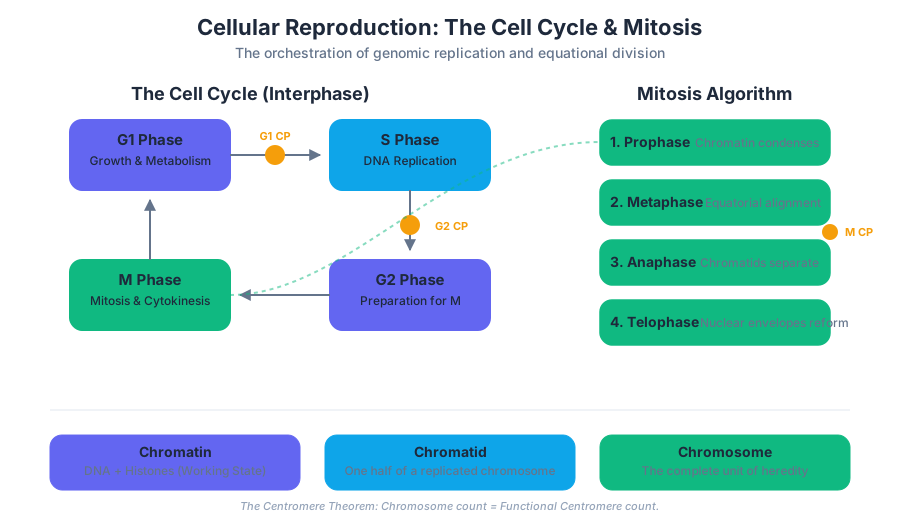
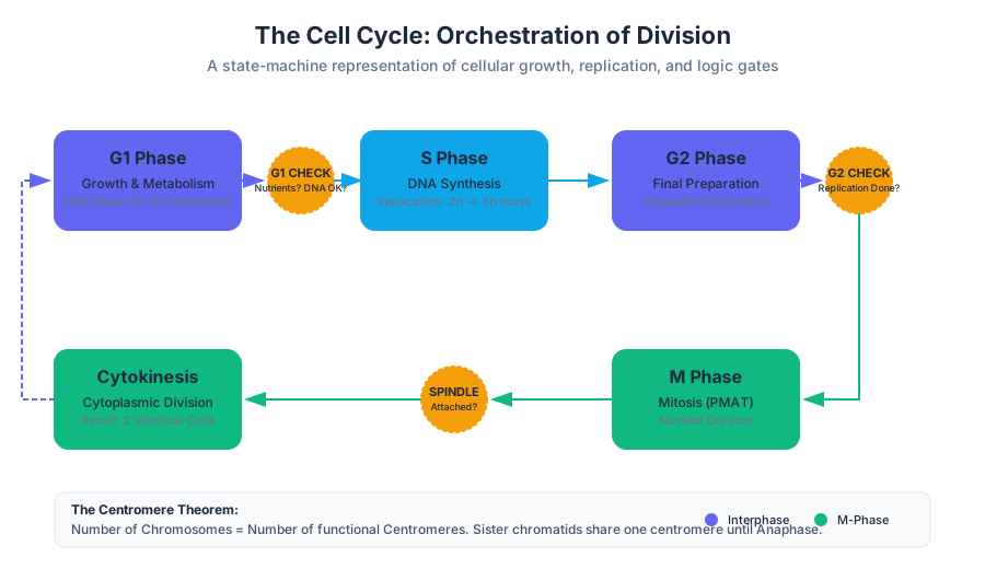
Foundations of Genetics: Mendelian Inheritance
Key concepts: Law of Segregation · Law of Independent Assortment · Punnett squares · Genotype vs. Phenotype
The laws of inheritance and the use of Punnett squares to predict genetic outcomes.
Foundations of Genetics: Mendelian Inheritance
The study of genetics began not with the discovery of DNA, but with the meticulous observation of patterns. Before the mid-19th century, the prevailing "Blending Theory" of inheritance suggested that parental traits mixed like paint—red and white flowers would produce pink offspring, and the original red and white traits would be lost forever. Gregor Mendel, an Augustinian friar, systematically dismantled this notion through his work with Pisum sativum (garden peas). His "Particulate Theory" proposed that traits are passed as discrete, heritable units that retain their identity across generations.
The Genotype-Phenotype Distinction
To understand Mendelian inheritance, one must first master the distinction between the physical expression of a trait and the underlying genetic composition. This duality is the cornerstone of modern biological analysis.
Definition: The Phenotype is the observable physical or physiological trait of an organism (e.g., purple flowers). The Genotype is the specific genetic makeup or set of alleles that determines that phenotype (e.g., Pp).
In Mendel's system, traits are governed by alleles—alternative versions of a gene found at the same locus (position) on homologous chromosomes.
| Term | Definition | Example (Pea Plants) |
|---|---|---|
| Allele | A variant form of a specific gene. | P (Purple) vs. p (White) |
| Homozygous | Having two identical alleles for a particular gene. | PP (Dominant) or pp (Recessive) |
| Heterozygous | Having two different alleles for a particular gene. | Pp |
| Dominant | An allele that masks the expression of a recessive allele. | Purple (P) |
| Recessive | An allele whose expression is masked by a dominant one. | White (p) |
The Mechanics of Dominance
Dominance is not a "strength" of an allele, but rather a functional relationship. In many cases, the dominant allele codes for a functional protein (like an enzyme that produces pigment), while the recessive allele is a "loss-of-function" mutation that produces a non-functional protein or none at all. In a heterozygote, the single functional allele often produces enough protein to achieve the full phenotype, making the trait appear dominant.
The First Law: The Law of Segregation
Mendel’s First Law, the Law of Segregation, describes how a single trait is passed from parents to offspring. It provides the mechanical explanation for why recessive traits can "disappear" in one generation and "reappear" in the next.
The Law of Segregation: During the formation of gametes (eggs and sperm), the two alleles for a heritable character segregate (separate) from each other and end up in different gametes.
The Derivation of the 3:1 Ratio
When Mendel crossed true-breeding purple-flowered plants (PP) with true-breeding white-flowered plants (pp), the $F_1$ (first filial) generation was 100% purple. However, when the $F_1$ plants were self-pollinated to produce the $F_2$ generation, the white trait reappeared in a consistent 3:1 ratio (Purple:White).
This ratio is a mathematical consequence of the random fusion of gametes. We can implement a simulation of this stochastic process to observe how these ratios emerge in large populations.
import random

def simulate_monohybrid_cross(parent1_genotype, parent2_genotype, trials=10000):
    """
    Simulates the Law of Segregation across a large number of offspring.
    Genotypes are represented as tuples, e.g., ('P', 'p').
    """
    results = {"PP": 0, "Pp": 0, "pp": 0}

    for _ in range(trials):
        # Each parent contributes one allele randomly
        gamete1 = random.choice(parent1_genotype)
        gamete2 = random.choice(parent2_genotype)

        # Sort to ensure 'Pp' and 'pP' are treated as the same genotype
        offspring = tuple(sorted((gamete1, gamete2)))
        genotype_str = "".join(offspring)
        results[genotype_str] += 1

    print(f"Simulation Results (n={trials}):")
    for gt, count in results.items():
        percentage = (count / trials) * 100
        print(f"Genotype {gt}: {count} ({percentage:.2f}%)")

# Crossing two F1 heterozygotes (Pp x Pp)
simulate_monohybrid_cross(('P', 'p'), ('P', 'p'))
The Second Law: The Law of Independent Assortment
While the Law of Segregation deals with single genes, the Law of Independent Assortment addresses the behavior of multiple genes relative to one another.
The Law of Independent Assortment: Each pair of alleles segregates independently of each other pair of alleles during gamete formation.
This law applies only to genes located on different chromosomes (or very far apart on the same chromosome). If two genes are "linked" (close together on the same chromosome), they tend to be inherited together, violating this law.
The Dihybrid Cross and the 9:3:3:1 Ratio
To prove this, Mendel performed a dihybrid cross, tracking two traits at once: seed color (Yellow Y vs. Green y) and seed shape (Round R vs. Wrinkled r). By crossing a double-homozygous dominant (YYRR) with a double-homozygous recessive (yyrr), he produced an $F_1$ generation of YyRr.
The $F_2$ generation produced four distinct phenotypes in a 9:3:3:1 ratio. This ratio is essentially the product of two independent 3:1 ratios: $(3:1) \times (3:1) = 9:3:3:1$.
Mathematical Derivation of Dihybrid Probabilities
We can express the probability of a specific phenotype using the Product Rule of probability, which states that the probability of two independent events occurring together is the product of their individual probabilities.
\begin{aligned}
&\text{Let } P(\text{Yellow}) = \frac{3}{4}, \quad P(\text{Green}) = \frac{1}{4} \\
&\text{Let } P(\text{Round}) = \frac{3}{4}, \quad P(\text{Wrinkled}) = \frac{1}{4} \\
\\
&P(\text{Yellow and Round}) = \frac{3}{4} \times \frac{3}{4} = \frac{9}{16} \\
&P(\text{Yellow and Wrinkled}) = \frac{3}{4} \times \frac{1}{4} = \frac{3}{16} \\
&P(\text{Green and Round}) = \frac{1}{4} \times \frac{3}{4} = \frac{3}{16} \\
&P(\text{Green and Wrinkled}) = \frac{1}{4} \times \frac{1}{4} = \frac{1}{16}
\end{aligned}
Punnett Squares: Probability Visualization
The Punnett Square is a visual grid used to predict the possible genetic outcomes of a cross. While simple for monohybrid crosses, it becomes a powerful tool for understanding the combinatorial nature of genetics.
Constructing a Punnett Square
- Identify the genotypes of the parents.
- Determine all possible gametes each parent can produce.
- Place the gametes of one parent across the top and the other down the side.
- Fill in the boxes by combining the row and column gametes.
| Gametes | YR | Yr | yR | yr |
|---|---|---|---|---|
| YR | YYRR | YYRr | YyRR | YyRr |
| Yr | YYRr | YYrr | YyRr | Yyrr |
| yR | YyRR | YyRr | yyRR | yyRr |
| yr | YyRr | Yyrr | yyRr | yyrr |
Beyond the Square: The Branch Diagram
For trihybrid crosses or higher, Punnett squares become unwieldy (a trihybrid square has 64 boxes). Instead, we use the Branch Diagram or Probability Method. To find the probability of a YyRrPp genotype from a YyRrPp x YyRrPp cross:
- Probability of Yy = 1/2
- Probability of Rr = 1/2
- Probability of Pp = 1/2
- Total Probability = $1/2 \times 1/2 \times 1/2 = 1/8$.
Practical Application: Pedigree Analysis and Data Management
In modern genetics, Mendelian principles are used to track disease inheritance in humans. Because we cannot perform controlled crosses on humans, we use pedigrees (family trees) to deduce genotypes.
When managing large-scale genetic data, researchers use relational databases to track phenotypes and genotypes across generations. Below is a SQL schema designed to represent Mendelian relationships and trait inheritance.
-- Schema for a Genetic Research Database
CREATE TABLE Organisms (
    organism_id INT PRIMARY KEY,
    species_name VARCHAR(100),
    generation_label VARCHAR(10), -- P, F1, F2
    parent1_id INT,
    parent2_id INT,
    FOREIGN KEY (parent1_id) REFERENCES Organisms(organism_id),
    FOREIGN KEY (parent2_id) REFERENCES Organisms(organism_id)
);

CREATE TABLE Traits (
    trait_id INT PRIMARY KEY,
    trait_name VARCHAR(50) -- e.g., 'Flower Color'
);

CREATE TABLE Genotypes (
    organism_id INT,
    trait_id INT,
    allele_1 CHAR(1),
    allele_2 CHAR(1),
    PRIMARY KEY (organism_id, trait_id),
    FOREIGN KEY (organism_id) REFERENCES Organisms(organism_id),
    FOREIGN KEY (trait_id) REFERENCES Traits(trait_id)
);

-- Query to find all offspring of a specific cross with a recessive phenotype
SELECT o.organism_id, g.allele_1, g.allele_2
FROM Organisms o
JOIN Genotypes g ON o.organism_id = g.organism_id
WHERE g.allele_1 = 'p' AND g.allele_2 = 'p'
AND (o.parent1_id = 101 AND o.parent2_id = 102);
Common Pitfalls and Misconceptions
Even at the foundational level, Mendelian genetics is often misunderstood.
- The "Dominant is Common" Fallacy: A dominant allele is not necessarily more common in a population than a recessive one. For example, polydactyly (extra fingers/toes) is caused by a dominant allele, but it is rare in the human population.
- The Gambler's Fallacy: If two heterozygous parents have three children with the dominant phenotype, the fourth child is not "due" to be recessive. Each fertilization event is an independent probability event ($P=1/4$ for recessive).
- Phenotype $\neq$ Genotype: You cannot always determine the genotype by looking at the phenotype. A purple flower could be PP or Pp. To distinguish them, Mendel used a Testcross—crossing the unknown individual with a homozygous recessive (pp).
| Scenario | Result of Testcross (with pp) | Conclusion |
|---|---|---|
| All offspring are Purple | 100% Pp | Unknown was PP |
| 50% Purple, 50% White | 50% Pp, 50% pp | Unknown was Pp |
Extensions of Mendelian Genetics
While Mendel's laws are the "laws of physics" for genetics, real-world biology often adds layers of complexity.
- Incomplete Dominance: The $F_1$ phenotype is a blend (e.g., Pink snapdragons from Red and White parents). Note that the alleles still segregate; the red and white traits reappear in the $F_2$.
- Codominance: Both alleles are expressed equally (e.g., AB blood type).
- Pleiotropy: One gene affects multiple phenotypic traits (e.g., the gene for sickle-cell anemia affects hemoglobin shape, malaria resistance, and organ health).
- Polygenic Inheritance: Multiple genes contribute to a single phenotype, creating a continuous spectrum (e.g., human skin color or height).
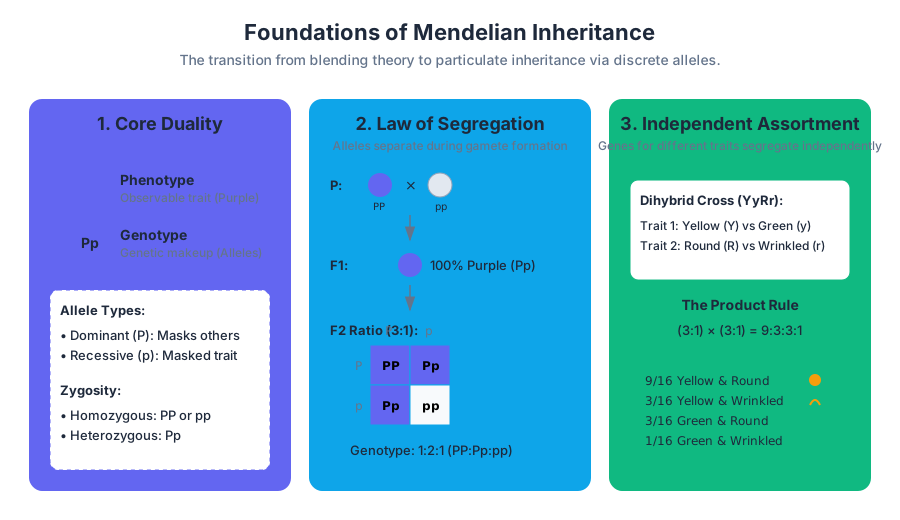
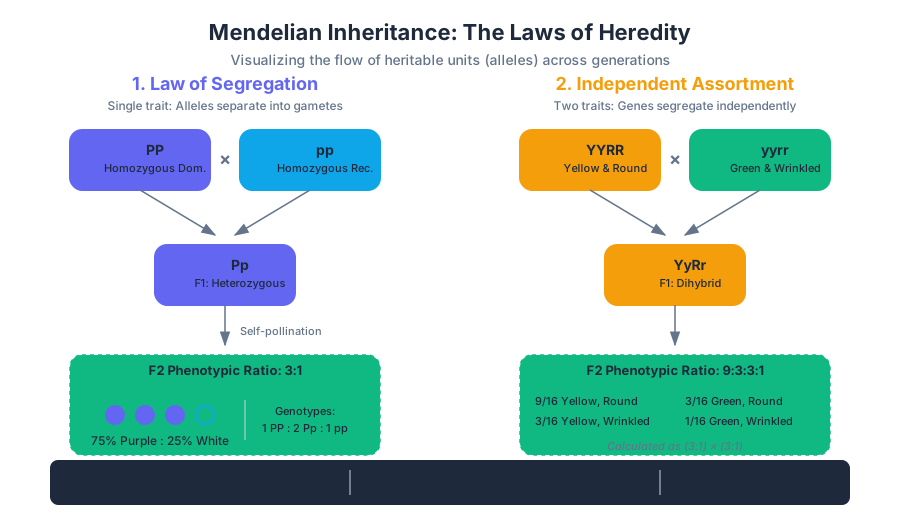
Complex Inheritance and Pedigree Analysis
Key concepts: Incomplete dominance · Codominance · Sex-linked traits · Pedigrees · Polygenic traits
Exploring genetic patterns that go beyond simple dominance and recessiveness.
Complex Inheritance and Pedigree Analysis
While Gregor Mendel’s work with Pisum sativum established the fundamental laws of segregation and independent assortment, the biological reality of inheritance is rarely as binary as "purple vs. white." In the century following Mendel, geneticists discovered that the relationship between genotype and phenotype is often modulated by dosage effects, multi-locus interactions, and chromosomal positioning. This article explores the sophisticated mechanisms of non-Mendelian inheritance and the analytical frameworks used to trace these traits through biological lineages.
The Spectrum of Dominance: Beyond Binary Traits
In classical Mendelian genetics, the dominant allele completely masks the recessive one. However, at the molecular level, dominance is a description of the phenotypic manifestation of heterozygosity, not an inherent property of an allele itself.
Incomplete Dominance
Incomplete dominance occurs when the phenotype of the heterozygote is an intermediate blend between the two homozygotes. This is typically a result of a "dosage effect," where a single functional allele cannot produce enough protein product to achieve the full homozygous phenotype.
Definition: Haploinsufficiency A situation where the total level of a gene product (protein) produced by a single functional allele is insufficient to maintain the normal (wild-type) function, leading to an intermediate or altered phenotype.
A classic example is the snapdragon (Antirrhinum majus). Crossing a homozygous red flower ($C^R C^R$) with a homozygous white flower ($C^W C^W$) results in pink offspring ($C^R C^W$). Here, the $C^R$ allele produces red pigment, but one copy is insufficient to saturate the petal tissue, resulting in a diluted pink appearance.
Codominance
In codominance, both alleles in the heterozygote are fully expressed, and neither masks the other. The resulting phenotype is not a blend, but a simultaneous display of both parental traits.
The most prominent human example is the ABO blood group system. The $I^A$ and $I^B$ alleles are codominant to each other, while both are dominant over the $i$ allele. An individual with the $I^A I^B$ genotype expresses both A and B antigens on the surface of their red blood cells.
| Feature | Complete Dominance | Incomplete Dominance | Codominance |
|---|---|---|---|
| Heterozygote Phenotype | Identical to dominant homozygote | Intermediate (blend) of parents | Both parental traits visible |
| Molecular Basis | One allele produces enough protein | Product dosage is insufficient | Both alleles produce distinct products |
| F2 Phenotypic Ratio | 3:1 | 1:2:1 | 1:2:1 |
| Example | Mendel's peas (Purple/White) | Snapdragon color (Pink) | Human AB blood type |
Sex-Linked Inheritance: The Chromosomal Asymmetry
Inheritance patterns shift dramatically when the gene of interest resides on a sex chromosome ($X$ or $Y$ in humans). Because males ($XY$) and females ($XX$) possess different "doses" of these chromosomes, the standard rules of autosomal probability do not apply.
X-Linked Traits
The X chromosome is significantly larger than the Y chromosome and carries thousands of genes unrelated to sex determination. Because males have only one X chromosome, they are hemizygous for X-linked traits.
- Recessive X-linked traits: More common in males. A male only needs one copy of the recessive allele (from his mother) to express the trait. A female needs two copies (one from each parent).
- Dominant X-linked traits: A father will pass the trait to all of his daughters but none of his sons.
Dosage Compensation and X-Inactivation
To prevent females from having twice as many X-linked gene products as males, placental mammals undergo X-inactivation. Early in embryonic development, one X chromosome in every female cell is randomly condensed into a transcriptionally inactive structure called a Barr body.
This creates a "genetic mosaic." For example, in calico cats, the gene for fur color is on the X chromosome. Depending on which X is inactivated in a specific patch of skin cells, the fur will be black or orange.
Mathematical Derivation of X-Linked Frequency
If the frequency of an X-linked recessive allele in a population is $q$, the probability of the phenotype appearing in the population is:
- In males: $P(m) = q$
- In females: $P(f) = q^2$
Since $q$ is usually a fraction (e.g., $0.08$ for color blindness), $q^2$ is significantly smaller ($0.0064$), explaining the sex disparity in disorders like Hemophilia A.
# Simulation of X-linked recessive inheritance over generations
import random

class Individual:
    def __init__(self, sex, genotype):
        self.sex = sex # 'M' or 'F'
        self.genotype = genotype # e.g., ['X_H', 'Y'] or ['X_H', 'X_h']

def produce_offspring(mother, father):
    m_allele = random.choice(mother.genotype)
    f_allele = random.choice(father.genotype)

    # Determine sex based on father's contribution
    offspring_genotype = [m_allele, f_allele]
    sex = 'F' if 'X' in f_allele and 'X' in m_allele else 'M'

    # Standardize genotype representation
    if sex == 'M':
        # Ensure Y is always the second element
        if 'Y' in offspring_genotype[0]:
            offspring_genotype = [offspring_genotype[1], offspring_genotype[0]]

    return Individual(sex, offspring_genotype)

# Example: Carrier Mother (X_H, X_h) and Unaffected Father (X_H, Y)
mother = Individual('F', ['X_H', 'X_h'])
father = Individual('M', ['X_H', 'Y'])

results = {"Affected Male": 0, "Normal Male": 0, "Carrier Female": 0, "Normal Female": 0}

for _ in range(10000):
    child = produce_offspring(mother, father)
    if child.sex == 'M':
        if 'X_h' in child.genotype: results["Affected Male"] += 1
        else: results["Normal Male"] += 1
    else:
        if 'X_h' in child.genotype: results["Carrier Female"] += 1
        else: results["Normal Female"] += 1

print(f"Simulation Results (10k iterations): {results}")
Polygenic Inheritance and Quantitative Genetics
Many traits do not fall into discrete categories but exist on a continuum (e.g., human height, skin pigmentation, or crop yield). These are polygenic traits, controlled by the cumulative effect of multiple genes, often interacting with environmental factors.
The Additive Model
In a simple polygenic model, each "active" allele contributes a specific "unit" to the phenotype. If three genes ($A, B, C$) control height, an individual with genotype $AABBCC$ would be the tallest, while $aabbcc$ would be the shortest.
The Bell Curve (Normal Distribution)
As the number of genes controlling a trait increases, the number of possible phenotypic variations increases exponentially, following a binomial distribution that approximates a Normal (Gaussian) Distribution.
f(x | \mu, \sigma^2) = \frac{1}{\sqrt{2\pi\sigma^2}} e^{ -\frac{(x-\mu)^2}{2\sigma^2} }
In this context:
- $\mu$ (Mean): The average phenotype produced by the most common combinations of alleles.
- $\sigma$ (Standard Deviation): Represents the phenotypic variance caused by both genetic diversity and environmental "noise."
| Property | Monogenic (Mendelian) | Polygenic (Quantitative) |
|---|---|---|
| Number of Genes | Single gene | Multiple genes (2 to hundreds) |
| Phenotypic Variation | Discrete (Discontinuous) | Continuous |
| Environmental Influence | Usually low | High |
| Analysis Method | Punnett Squares / Pedigrees | Statistical Analysis / QTL Mapping |
| Examples | Cystic Fibrosis, Pea Color | Height, Skin Tone, IQ |
Pedigree Analysis: The Logic of Genetic Inference
A pedigree is a graphical representation of a family’s genetic history. By analyzing the distribution of a trait across generations, we can determine the mode of inheritance (dominant vs. recessive, autosomal vs. sex-linked).
Standard Symbols
- Squares: Males
- Circles: Females
- Shaded: Affected individuals
- Unshaded: Unaffected individuals
- Horizontal Line: Mating
- Vertical Line: Offspring
Heuristics for Pattern Recognition
- Autosomal Recessive:
- Trait often skips generations.
- Two unaffected parents can have an affected child (both parents are carriers).
- If both parents are affected, all children must be affected.
- Autosomal Dominant:
- Trait appears in every generation (does not skip).
- Affected children must have at least one affected parent.
- Two affected parents can have an unaffected child (if both parents are heterozygous).
- X-Linked Recessive:
- Significantly more males are affected than females.
- An affected mother will have 100% affected sons.
- The trait is never passed from father to son (sons inherit Y from father).
- X-Linked Dominant:
- An affected father will pass the trait to all of his daughters and none of his sons.
- Affected females can pass the trait to both sons and daughters.
Theorem: The Exclusion Principle In pedigree analysis, the mode of inheritance is often determined by excluding impossible patterns rather than proving a single one. For instance, if a daughter expresses a recessive trait but her father does not, the trait cannot be X-linked recessive.
Pedigree Data Representation
In computational biology, pedigrees are often stored as relational tables or adjacency lists to allow for automated risk assessment.
-- Query to identify potential carriers of an autosomal recessive trait
-- Logic: An individual is a carrier if they are unaffected BUT have an affected child
-- OR if they are unaffected but have an affected parent.

WITH AffectedIndividuals AS (
    SELECT person_id FROM pedigree_table WHERE phenotype = 'Affected'
),
ParentsOfAffected AS (
    SELECT DISTINCT father_id AS parent_id FROM pedigree_table WHERE person_id IN (SELECT person_id FROM AffectedIndividuals)
    UNION
    SELECT DISTINCT mother_id AS parent_id FROM pedigree_table WHERE person_id IN (SELECT person_id FROM AffectedIndividuals)
)
SELECT p.person_id, p.name
FROM pedigree_table p
JOIN ParentsOfAffected poa ON p.person_id = poa.parent_id
WHERE p.phenotype = 'Unaffected';
Advanced Concepts: Epistasis and Pleiotropy
To fully master complex inheritance, one must look at how genes interact with each other and how a single gene can have multiple effects.
Epistasis
Epistasis occurs when the effect of one gene is dependent on the presence of one or more "modifier genes." Essentially, one gene masks or interferes with the expression of another.
Example: Labrador Retriever Coat Color.
- Gene 1 ($B$): Determines pigment color (Black $B$ vs. Brown $b$).
- Gene 2 ($E$): Determines if pigment is deposited in the hair ($E$ for yes, $e$ for no).
- If a dog has the genotype $ee$, it will be yellow regardless of whether its $B$ alleles are black or brown. The $e$ gene is epistatic to the $B$ gene.
Pleiotropy
Pleiotropy is the phenomenon where a single gene influences multiple, seemingly unrelated phenotypic traits. Most genetic diseases are pleiotropic. For example, Sickle Cell Anemia is caused by a single mutation in the hemoglobin gene, but it results in physical weakness, organ damage, brain damage, and even resistance to malaria.
Common Pitfalls in Genetic Analysis
- Small Sample Size: In human pedigrees, the number of offspring is usually too small to see perfect Mendelian ratios (e.g., a 3:1 ratio). Statistical significance is difficult to achieve without large multi-generational data.
- Lethal Alleles: Some genotypic combinations (usually homozygous dominant or recessive) are lethal in utero. This "removes" a class of offspring from the observed data, shifting the ratios (e.g., a 2:1 ratio instead of 3:1).
- Incomplete Penetrance: An individual may carry the dominant genotype but not express the phenotype due to environmental factors or other modifier genes.
- Variable Expressivity: Individuals with the same genotype may show the trait to different degrees of severity.
Summary of Inheritance Patterns
To conclude, inheritance is a multi-layered system of information transfer. While Mendel provided the "syntax," complex inheritance provides the "context." Understanding the nuances of dominance, sex-linkage, and polygenic interaction is essential for modern genomic medicine, agricultural optimization, and evolutionary biology.
| Pattern | Key Identifier | Molecular Mechanism |
|---|---|---|
| Incomplete Dominance | 1:2:1 Phenotypic Ratio | Enzyme saturation/Dosage |
| Codominance | Both traits expressed | Independent protein production |
| X-Linked Recessive | Male bias in pedigree | Hemizygosity in males |
| Polygenic | Continuous distribution | Additive effect of multiple loci |
| Epistasis | One gene masks another | Pathway-level interference |
| Pleiotropy | One gene, many effects | Protein used in multiple tissues |
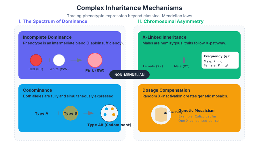
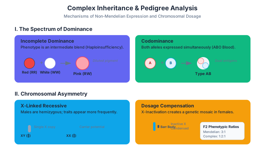
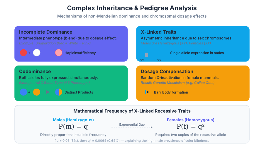
Source Materials
Study High School Biology with AI — Free on Lykke
Sign up for free to generate personalized flashcards, quizzes, and study guides from this course. Chat with an AI tutor that knows the material.
Get Started FreeView this course wiki on Lykke · Browse all public course wikis