Finance Theory I
Institution: MIT
48 study materials · 10 sections
Finance Theory I provides a rigorous introduction to the fundamental principles of modern financial economics and investment management. The course focuses on the valuation of financial assets, the relationship between risk and return, and the strategic allocation of capital in global markets. Students explore core frameworks including Net Present Value (NPV), the Capital Asset Pricing Model (CAPM), and the Efficient Markets Hypothesis, while also addressing contemporary developments like Behavioral Finance and the role of AI in fiduciary guidance.
Course Sections
Foundations of Finance and Time Value of Money
Key concepts: Present Value (PV) · Net Present Value (NPV) · Perpetuities and Annuities · Compounding Conventions · Leverage Ratio
Introduction to the fundamental principles of financial valuation, focusing on the time value of money and cash flow analysis.
Foundations of Finance and Time Value of Money
Overview
This section establishes the bedrock of financial theory: the axiom that a dollar today is worth more than a dollar tomorrow. This is not merely a rule of thumb but a mathematical necessity derived from the opportunity cost of capital. In this module, we move beyond simple accounting to financial economics, introducing the tools required to value sequences of cash flows across time and under conditions of certainty. We will explore how to collapse a complex future into a single, comparable number today.
AI_SVGI_SVG## Key Concepts
- Present Value (PV) & Net Present Value (NPV): The core metrics for determining the current worth of future cash flows. NPV is the primary tool for decision-making, representing the difference between the present value of cash inflows and outflows.
- Perpetuities and Annuities: Specialized formulas for valuing constant cash flows that continue forever (perpetuities) or for a fixed period (annuities).
- Compounding Conventions: Understanding how interest rates are applied over different frequencies (annual, semi-annual, continuous) and the calculation of the Effective Annual Rate (EAR).
- Leverage Ratio: An introduction to how debt influences financial positions and returns, acting as a multiplier for both gains and losses.
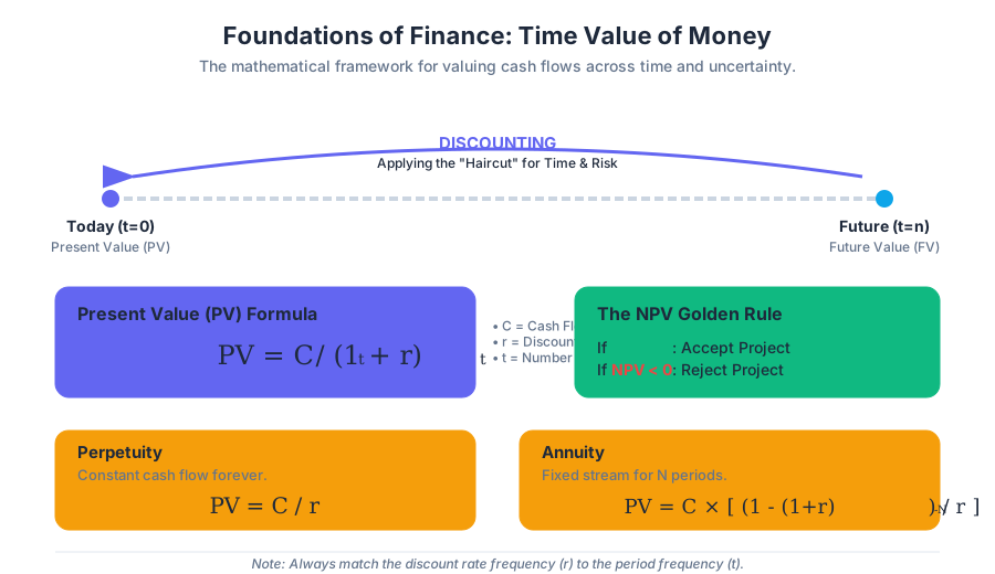
### Present Value (PV) and the Discount Factor
What it is
Present Value (PV) is the current value of a future sum of money or stream of cash flows given a specified rate of return. It represents the amount of money that would need to be invested today, at a given interest rate, to generate that future amount.
Mathematically, for a single cash flow $C_t$ occurring at time $t$, the Present Value is: $$PV = \frac{C_t}{(1+r)^t}$$ Where:
- $C_t$ = Cash flow at time $t$
- $r$ = Discount rate (opportunity cost of capital)
- $t$ = Number of periods
Why it matters
The PV formula is the "universal translator" of finance. It allows us to compare cash flows that occur at different points in time by bringing them all to a common denominator: "today's dollars." Without PV, we cannot objectively compare a $1,000 payment today versus a $1,200 payment in three years.
How it works: The Discount Factor
We often define the Discount Factor (DF) as the present value of $1 received at time $t$: $$DF_t = \frac{1}{(1+r)^t}$$ The discount factor is always less than 1 (assuming positive interest rates), reflecting the "haircut" we apply to future money to account for the time value.
Concrete Example
Suppose you are promised $5,000 in 3 years. If the prevailing market interest rate for an investment of similar risk is 6%, what is this promise worth today?
- $C_3 = 5,000$
- $r = 0.06$
- $t = 3$ $$PV = \frac{5,000}{(1.06)^3} = \frac{5,000}{1.191016} \approx \text{\textdollar}4,198.10$$
Common Pitfalls
- Mismatched Rates and Periods: If the cash flow occurs in 6 months, but the rate $r$ is annual, you must adjust $t$ to 0.5 or convert $r$ to a semi-annual rate.
- Ignoring Risk: The discount rate $r$ must reflect the risk of the cash flow. Using a risk-free rate for a high-risk startup investment will lead to a massive overvaluation.
### Net Present Value (NPV): The Golden Rule of Decision Making
What it is
Net Present Value (NPV) is the sum of the present values of all cash flows (both positive and negative) associated with an investment or project. It measures the net wealth created by an investment.
$$NPV = -C_0 + \sum_{t=1}^{T} \frac{C_t}{(1+r)^t}$$ Where $C_0$ is the initial investment (outlay).
Why it matters
NPV is the "Gold Standard" for capital budgeting. Unlike other metrics like the Internal Rate of Return (IRR) or Payback Period, NPV directly measures the expected increase in shareholder wealth.
The NPV Rule: Accept all projects with a positive NPV ($NPV > 0$) and reject those with a negative NPV. If comparing mutually exclusive projects, choose the one with the highest NPV.
Comparison of Decision Metrics
| Metric | Definition | Decision Rule | Major Flaw |
|---|---|---|---|
| NPV | Present value of all net cash flows | Accept if $> 0$ | Requires accurate $r$ estimation |
| IRR | The rate $r$ where $NPV = 0$ | Accept if $IRR >$ cost of cap | Can have multiple solutions; ignores scale |
| Payback | Time to recover initial outlay | Accept if $< X$ years | Ignores TVM and cash flows after payback |
| Profitability Index | Ratio of PV of inflows to Outlay | Accept if $> 1$ | Can fail when choosing between mutually exclusive projects |
Concrete Example
A company is considering a machine that costs $100,000 today ($C_0$). It is expected to generate $40,000 per year for 3 years. The discount rate is 10%.
- $PV(C_1) = 40,000 / 1.10 = 36,363.64$
- $PV(C_2) = 40,000 / 1.10^2 = 33,057.85$
- $PV(C_3) = 40,000 / 1.10^3 = 30,052.59$
- $Sum\ of\ PVs = 99,474.08$
- $NPV = 99,474.08 - 100,000 = -\text{\textdollar}525.92$ Decision: Reject the project. It destroys $525.92 of value.
### Perpetuities and Annuities
In many financial applications, we deal with constant streams of cash flows. Rather than discounting each flow individually, we use closed-form mathematical shortcuts.
1. Perpetuities
A Perpetuity is a constant stream of cash flows ($C$) that continues forever. Formula: $$PV_{perpetuity} = \frac{C}{r}$$ Derivation: This is the limit of a geometric series $\sum_{t=1}^{\infty} \frac{C}{(1+r)^t}$. As $t \to \infty$, the sum converges to $C/r$.
2. Growing Perpetuities
If the cash flow grows at a constant rate $g$ forever: $$PV_{growing\ perpetuity} = \frac{C_1}{r - g}$$ Constraint: $r$ must be greater than $g$. If $g \ge r$, the value is infinite.
3. Annuities
An Annuity is a stream of $N$ equal cash flows $C$ paid at regular intervals for a fixed period. Formula: $$PV_{annuity} = C \times \left[ \frac{1}{r} - \frac{1}{r(1+r)^N} \right]$$ The term in the brackets is often called the Annuity Factor.
4. Growing Annuities
A stream of $N$ cash flows growing at rate $g$: $$PV_{growing\ annuity} = \frac{C_1}{r-g} \left[ 1 - \left( \frac{1+g}{1+r} \right)^N \right]$$
Comparison of Stream Types
| Type | Cash Flow Pattern | Duration | Primary Use Case |
|---|---|---|---|
| Level Perpetuity | $C, C, C, ...$ | Infinite | Preferred stock, Consols |
| Growing Perpetuity | $C, C(1+g), ...$ | Infinite | Dividend Discount Model (Mature firms) |
| Level Annuity | $C, C, ...$ | $N$ periods | Mortgages, Car loans, Lease payments |
| Growing Annuity | $C, C(1+g), ...$ | $N$ periods | Retirement savings with salary growth |
AI_DEMOI_DEMO--
### Compounding Conventions and EAR
What it is
Interest rates are rarely as simple as "10% per year." The frequency with which interest is calculated (compounding) significantly changes the actual interest paid or earned.
- Annual Percentage Rate (APR): The "stated" or "nominal" rate. It does not account for compounding within the year.
- Effective Annual Rate (EAR): The actual rate earned/paid after accounting for compounding.
The Formula
To convert an APR to an EAR with $m$ compounding periods per year: $$EAR = \left( 1 + \frac{APR}{m} \right)^m - 1$$
Continuous Compounding
As $m$ approaches infinity, we reach Continuous Compounding. This is used extensively in derivatives pricing (e.g., Black-Scholes). $$EAR = e^{APR} - 1$$ $$PV = C_t \times e^{-rt}$$
Compounding Frequency Comparison (Stated Rate = 10%)
| Frequency | $m$ | Formula | EAR |
|---|---|---|---|
| Annual | 1 | $(1 + 0.10/1)^1 - 1$ | 10.00% |
| Semi-Annual | 2 | $(1 + 0.10/2)^2 - 1$ | 10.25% |
| Quarterly | 4 | $(1 + 0.10/4)^4 - 1$ | 10.38% |
| Monthly | 12 | $(1 + 0.10/12)^{12} - 1$ | 10.47% |
| Daily | 365 | $(1 + 0.10/365)^{365} - 1$ | 10.516% |
| Continuous | $\infty$ | $e^{0.10} - 1$ | 10.517% |
Implementation in Code
The following Python snippet demonstrates how to calculate NPV and compare EAR across different frequencies.
import math

def calculate_ear(apr, m=None, continuous=False):
    """Calculates Effective Annual Rate."""
    if continuous:
        return math.exp(apr) - 1
    return (1 + apr / m)**m - 1

def calculate_npv(rate, cash_flows):
    """Calculates Net Present Value for a list of cash flows."""
    return sum(cf / (1 + rate)**t for t, cf in enumerate(cash_flows))

# Example Usage
stated_rate = 0.08
flows = [-1000, 400, 400, 400] # Initial outlay of 1000, 3 years of 400

print(f"EAR (Monthly): {calculate_ear(stated_rate, m=12):.4%}")
print(f"EAR (Continuous): {calculate_ear(stated_rate, continuous=True):.4%}")
print(f"Project NPV: ${calculate_npv(stated_rate, flows):.2f}")
### Leverage Ratio
What it is
Leverage refers to the use of borrowed money (debt) to finance the purchase of assets, with the expectation that the income or capital gain from the new asset will exceed the cost of borrowing.
The Leverage Ratio can be defined in several ways, but a common version is: $$Leverage = \frac{Total\ Assets}{Equity}$$ Or the Debt-to-Equity Ratio: $$D/E = \frac{Total\ Debt}{Total\ Equity}$$
Why it matters
Leverage is a double-edged sword. It magnifies the Return on Equity (ROE). If the return on assets (ROA) is higher than the interest rate on debt, leverage increases ROE. If ROA is lower than the interest rate, leverage accelerates losses.
How it works: The ROE Formula
$$ROE = \frac{Net\ Income}{Equity} = [ROA + (ROA - Interest\ Rate) \times \frac{Debt}{Equity}] \times (1 - Tax\ Rate)$$
Concrete Example: The Power of Leverage
Imagine two investors, A and B, both buying a $1,000,000 building.
- Investor A (No Leverage): Pays $1M cash.
- Investor B (Leveraged): Pays $200k cash (Equity) and borrows $800k at 5% interest.
Scenario: Building value increases by 10% ($100k gain)
- Investor A: $100k gain on $1M investment = 10% Return.
- Investor B: $100k gain - $40k interest = $60k profit. $60k profit on $200k investment = 30% Return.
Scenario: Building value decreases by 10% ($100k loss)
- Investor A: $100k loss on $1M investment = -10% Return.
- Investor B: $100k loss + $40k interest = $140k total loss. $140k loss on $200k investment = -70% Return.
Common Pitfalls
- Ignoring the Cost of Financial Distress: High leverage increases the probability of bankruptcy. The "cost" of leverage isn't just the interest rate; it's the risk of total loss.
- Volatility Miscalculation: Investors often underestimate how quickly a small dip in asset prices can wipe out equity when leverage is 10x or 20x (common in pre-2008 investment banking).
AI_FLASHCARDSI_FLASHCARDS Present Value (PV): $PV = C / (1+r)^t$
- Net Present Value (NPV): Sum of all discounted cash flows; $NPV > 0$ means value creation.
- Perpetuity: $PV = C / r$
- Annuity Factor: $[1/r - 1/(r(1+r)^N)]$
- EAR (Periodic): $(1 + APR/m)^m - 1$
- EAR (Continuous): $e^{APR} - 1$
- Leverage Ratio: Total Assets / Equity; magnifies both risk and reward.
- Opportunity Cost of Capital: The expected return foregone by investing in a project rather than in comparable financial securities.
AI_QUIZI_QUIZ. Scenario: You are offered a choice between $10,000 today or $11,000 in one year. If the market interest rate is 12%, which should you choose?
- Answer: Choose $10,000 today. The PV of $11,000 is $11,000 / 1.12 = $9,821.43, which is less than $10,000.
- Concept: Why does the NPV rule dominate the IRR rule for mutually exclusive projects of different scales?
- Answer: Because IRR is a percentage and doesn't account for the absolute dollar value created. A 100% return on $1 is worse than a 10% return on $1,000,000.
- Calculation: If a bank quotes an APR of 12% compounded monthly, what is the EAR?
- Answer: $(1 + 0.12/12)^{12} - 1 = (1.01)^{12} - 1 \approx 12.68%$.
- Theory: What happens to the PV of an annuity if the interest rate $r$ increases?
- Answer: The PV decreases. Since $r$ is in the denominator of the discount factor, a higher $r$ reduces the value of future cash flows.
- Leverage: If a firm has a Debt-to-Equity ratio of 1.0 and its ROA is 8% while its interest rate is 5%, what is its ROE (ignoring taxes)?
- Answer: $ROE = 8% + (8% - 5%) \times 1.0 = 11%$.
AI_STUDY_GUIDEI_STUDY_GUIDE## Study Guide: Foundations of Finance
1. Fundamental Principles
- Time Value of Money (TVM): Understand that the value of money is a function of time, risk, and opportunity cost.
- The Law of One Price: In efficient markets, two assets with the same cash flows must have the same price. This underlies all PV calculations.
2. Mathematical Mastery
- Practice converting between APR and EAR. This is a frequent source of error in exams and professional modeling.
- Memorize the Annuity and Perpetuity formulas. You should be able to derive the perpetuity formula using the sum of a geometric series.
- Understand the Relationship between $r$ and $PV$: They are inversely related. Understand the relationship between $t$ and $PV$: They are also inversely related.
3. Decision Criteria
- Be able to calculate NPV for uneven cash flow streams.
- Explain why NPV is the superior decision metric compared to Payback, IRR, and Book Rate of Return.
- Know the conditions under which IRR fails (e.g., non-conventional cash flows, mutually exclusive projects).
4. Leverage and Risk
- Understand the Balance Sheet identity: $Assets = Liabilities + Equity$.
- Be able to calculate the impact of Leverage on ROE.
- Recognize that leverage does not create value in a frictionless world (Modigliani-Miller), but it changes the risk profile of the equity holders.
5. Real-World Applications
- Bond Pricing: A bond is simply an annuity (coupons) plus a single payment (par value).
- Stock Valuation: A stock can be modeled as a growing perpetuity of dividends.
- Mortgages: An amortizing loan is a level annuity.
Fixed-Income Securities
Key concepts: Coupon Bonds · Yield Curves · Spot and Forward Rates · Modified Duration · Law of One Price
Exploration of bond valuation, interest rate dynamics, and the term structure of interest rates.
Fixed-Income Securities
Fixed-income securities represent the bedrock of the global financial system. While equity markets often capture the public imagination, the fixed-income market—comprising government debt, corporate bonds, and securitized products—is significantly larger in terms of total notional value and serves as the primary mechanism for capital allocation and monetary policy transmission.
In this section, we move beyond the basic time-value-of-money (TVM) principles to explore the rigorous mechanics of debt instruments. We will define how these securities are priced, how their risks are quantified through duration and convexity, and how the "term structure" of interest rates provides a window into the market's collective expectation of the future.
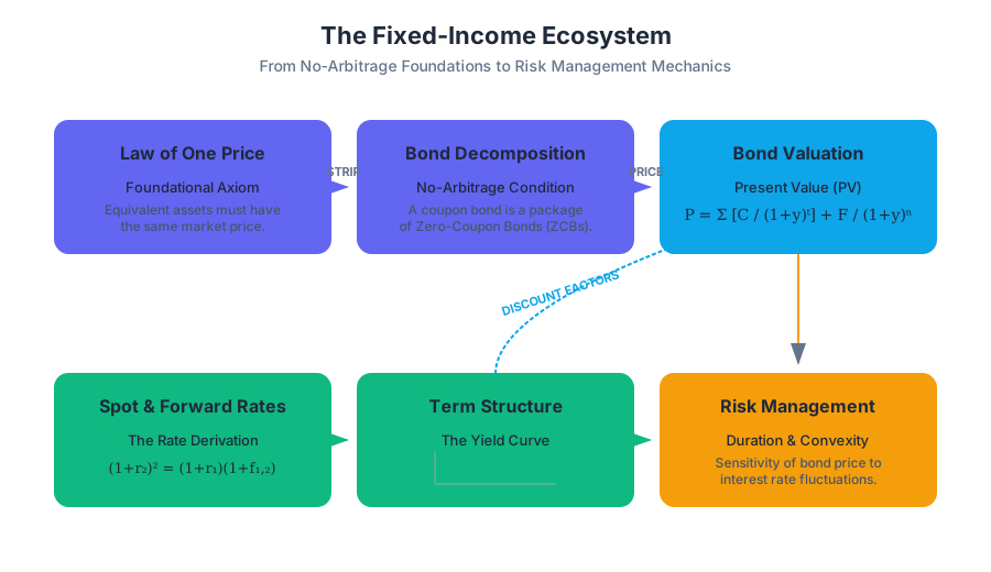
AI_SVGI_SVGThe Fixed-Income Ecosystem: A visualization showing the flow from the Law of One Price to Spot/Forward rates, leading to Bond Valuation and finally to Risk Management via Duration and Convexity.*
The Law of One Price and No-Arbitrage
The foundational axiom of modern finance is the Law of One Price (LoOP). It states that in a competitive market, if two assets are equivalent in all relevant aspects (specifically their cash flow timing and risk profile), they must have the same market price.
In the context of fixed-income, this implies that a complex security, such as a coupon-bearing bond, can be viewed as a "package" of simpler securities. Specifically, any bond can be decomposed into a series of Zero-Coupon Bonds (ZCBs).
Theorem: The No-Arbitrage Condition If a coupon bond provides cash flows $C_1, C_2, \dots, C_n$ at times $t_1, t_2, \dots, t_n$, and the market price of a ZCB maturing at time $t$ is $P(0, t)$, then the price of the coupon bond $P_{bond}$ must satisfy: $$P_{bond} = \sum_{i=1}^{n} C_i \cdot P(0, t_i)$$ If $P_{bond}$ were higher, an arbitrageur would sell the bond and buy the individual ZCBs (strips) to lock in a riskless profit. If lower, they would do the reverse.
Implications for Valuation
This principle allows us to value any fixed-income instrument without needing a single "interest rate." Instead, we use the specific discount factor relevant to each specific maturity.
Coupon Bonds: Mechanics and Valuation
A Coupon Bond is a debt instrument where the issuer (borrower) commits to making periodic interest payments (coupons) and returning the face value (principal) at maturity.
The Valuation Formula
The price of a bond is the present value (PV) of its future cash flows, discounted at the Yield to Maturity (YTM), denoted as $y$. For a bond with face value $F$, annual coupon rate $c$, and $n$ periods to maturity:
$$P = \sum_{t=1}^{n} \frac{C}{(1+y)^t} + \frac{F}{(1+y)^n}$$
Where $C = \frac{c \cdot F}{m}$ (if payments are $m$ times per year).
Bond Price Dynamics
The relationship between a bond's coupon rate and its YTM determines whether it trades at a premium or a discount.
| Relationship | Bond Status | Price vs. Face Value |
|---|---|---|
| Coupon Rate > YTM | Premium | $P > F$ |
| Coupon Rate < YTM | Discount | $P < F$ |
| Coupon Rate = YTM | Par | $P = F$ |
Worked Example: Pricing a Semi-Annual Bond
Consider a corporate bond with:
- Face Value ($F$): $1,000
- Coupon Rate: 6% (paid semi-annually)
- Maturity: 2 years
- YTM: 4% (annualized)
Step 1: Identify Parameters
- $C = (0.06 \times 1000) / 2 = \text{\textdollar}30$
- $n = 2 \times 2 = 4$ periods
- $y_{period} = 0.04 / 2 = 0.02$ (2%)
Step 2: Calculate PV $$P = \frac{30}{(1.02)^1} + \frac{30}{(1.02)^2} + \frac{30}{(1.02)^3} + \frac{1030}{(1.02)^4}$$ $$P = 29.41 + 28.83 + 28.27 + 951.55 = \text{\textdollar}1,038.06$$ The bond trades at a premium because the coupon (6%) is higher than the market required return (4%).
The Term Structure of Interest Rates
The Term Structure describes the relationship between interest rates and the time to maturity for a given class of bonds (usually risk-free government bonds). This is visualized through the Yield Curve.
Spot Rates vs. Forward Rates
To understand the term structure, we must distinguish between different types of rates:
- Spot Rate ($r_t$): The annualized interest rate agreed upon today for a loan that begins immediately and lasts for $t$ periods.
- Forward Rate ($f_{t, T}$): The interest rate agreed upon today for a loan that will begin at a future date $t$ and end at date $T$.
The Forward Rate Derivation
Under the No-Arbitrage assumption, the return from investing in a long-term spot contract must equal the return from rolling over a series of short-term contracts.
For a two-period horizon: $$(1 + r_2)^2 = (1 + r_1)(1 + f_{1,2})$$
Solving for the forward rate: $$f_{1,2} = \frac{(1 + r_2)^2}{(1 + r_1)} - 1$$
Yield Curve Theories
Why is the yield curve shaped the way it is? There are three primary economic explanations:
| Theory | Core Logic | Implications |
|---|---|---|
| Expectations Hypothesis | Long-term rates are the average of expected future short-term rates. | An upward slope means the market expects rates to rise. |
| Liquidity Preference | Investors demand a premium for the risk of locking up capital for longer periods. | The curve should naturally slope upward (Liquidity Premium). |
| Market Segmentation | Different investors (pension funds vs. banks) prefer different maturities. | Supply and demand in specific "buckets" determine the shape. |
AI_DEMOI_DEMOInteractive Yield Curve: A simulation where users can adjust inflation expectations and liquidity premiums to see how the Yield Curve shifts from Normal to Inverted.*
Interest-Rate Risk: Duration and Convexity
Bond prices move inversely to interest rates. However, not all bonds react with the same intensity. Duration is the primary metric used to quantify this sensitivity.
Macaulay Duration ($D_{mac}$)
Macaulay Duration is the weighted average time to receive the cash flows from a bond, measured in years.
$$D_{mac} = \frac{\sum_{t=1}^{n} t \cdot PV(CF_t)}{P}$$
Modified Duration ($D_{mod}$)
To find the actual percentage change in price for a given change in yield, we use Modified Duration:
$$D_{mod} = \frac{D_{mac}}{1 + y}$$
The Duration Rule: The approximate percentage change in a bond's price for a small change in yield ($\Delta y$) is: $$\frac{\Delta P}{P} \approx -D_{mod} \cdot \Delta y$$
Convexity: The Second-Order Effect
The relationship between bond prices and yields is not linear; it is convex. Duration is merely the first derivative (the slope) of the price-yield curve. For large interest rate moves, duration underestimates the price of the bond.
Convexity ($C$) accounts for the curvature. The more accurate price change formula is: $$\frac{\Delta P}{P} \approx -D_{mod} \cdot \Delta y + \frac{1}{2} C \cdot (\Delta y)^2$$
Comparison of Sensitivity Factors
| Factor | Effect on Duration | Effect on Interest Rate Risk |
|---|---|---|
| Higher Coupon | Decreases | Lower risk (capital returned faster) |
| Longer Maturity | Increases | Higher risk (more time for rates to fluctuate) |
| Higher YTM | Decreases | Lower risk (discounting dampens future CFs) |
Implementation: Bond Pricing and Risk Engine
In modern finance, these calculations are automated. Below is a high-signal Python implementation using numpy to calculate the price, Macaulay Duration, and Modified Duration of a bond.
import numpy as np

def calculate_bond_metrics(face_value, coupon_rate, ytm, years, freq=2):
    """
    Calculates Price, Macaulay Duration, and Modified Duration.
    freq: 1 for annual, 2 for semi-annual, 4 for quarterly.
    """
    periods = years * freq
    coupon_payment = (coupon_rate * face_value) / freq
    periodic_ytm = ytm / freq

    times = np.arange(1, periods + 1)
    cash_flows = np.array([coupon_payment] * (periods - 1) + [coupon_payment + face_value])

    # Discount factors: 1 / (1 + r)^t
    discount_factors = 1 / (1 + periodic_ytm)**times
    pv_cash_flows = cash_flows * discount_factors

    price = np.sum(pv_cash_flows)

    # Macaulay Duration in periods
    macaulay_duration_periods = np.sum(times * pv_cash_flows) / price
    macaulay_duration_years = macaulay_duration_periods / freq

    # Modified Duration
    modified_duration = macaulay_duration_years / (1 + periodic_ytm)

    return {
        "Price": round(price, 2),
        "Macaulay Duration": round(macaulay_duration_years, 3),
        "Modified Duration": round(modified_duration, 3)
    }

# Example: 10-year, 5% coupon bond, 4% YTM
metrics = calculate_bond_metrics(1000, 0.05, 0.04, 10)
print(metrics)
# Output: {'Price': 1081.76, 'Macaulay Duration': 7.989, 'Modified Duration': 7.832}
Common Pitfalls in Fixed-Income Analysis
- Ignoring Reinvestment Risk: The YTM calculation assumes all coupons are reinvested at the same YTM rate. In a falling-rate environment, the actual realized return will be lower than the YTM.
- Confusing Nominal and Real Rates: Fixed-income investors are highly sensitive to inflation. If nominal rates are 5% but inflation is 6%, the real return is negative.
- Duration Misapplication: Duration is only a local approximation. For large "shocks" to the yield curve (e.g., a 200 basis point move), failing to include convexity will lead to significant pricing errors.
- The "Pull to Par" Illusion: Investors often think discount bonds are "cheaper." However, the price appreciation toward par is simply a component of the YTM, not an excess return.
AI_FLASHCARDSI_FLASHCARDS Spot Rate: The yield on a zero-coupon bond for a specific maturity.
- Forward Rate: An interest rate set today for a loan occurring in the future.
- Yield to Maturity (YTM): The internal rate of return (IRR) of a bond's cash flows.
- Macaulay Duration: The weighted average time to receive cash flows.
- Modified Duration: A measure of price sensitivity to interest rate changes ($\Delta P/P$).
- Convexity: The measure of the curvature in the relationship between bond prices and yields.
- Law of One Price: The rule that identical cash flows must have identical prices.
AI_QUIZI_QUIZ. If the yield curve is inverted (short-term rates > long-term rates), what does the Expectations Hypothesis suggest about future interest rates? 2. A bond has a Modified Duration of 8.0. If interest rates rise by 50 basis points (0.50%), what is the approximate percentage change in the bond's price? 3. Why does a zero-coupon bond have a Macaulay Duration exactly equal to its maturity? 4. Between a 5% coupon bond and a 0% coupon bond, both with 10 years to maturity, which has higher interest rate risk? 5. If a bond's price is $1,050 and its face value is $1,000, is the YTM higher or lower than the coupon rate?
AI_STUDY_GUIDEI_STUDY_GUIDE*Key Formulas to Memorize:**
- Bond Price: $P = \sum \frac{C}{(1+y)^t} + \frac{F}{(1+y)^n}$
- Forward Rate (1-period): $f_{t, t+1} = \frac{(1+r_{t+1})^{t+1}}{(1+r_t)^t} - 1$
- Duration Rule: $\Delta P/P \approx -D_{mod} \cdot \Delta y$
- Modified Duration: $D_{mod} = D_{mac} / (1+y)$
Conceptual Checklist:
- Can I explain why bond prices and yields move inversely?
- Do I understand how to bootstrap a spot curve from coupon bond prices?
- Can I distinguish between the three main yield curve theories?
- Do I know when to use duration vs. when convexity is required?
- Can I apply the Law of One Price to identify an arbitrage opportunity?
Suggested Practice:
- Calculate the price of a 5-year bond with a 4% coupon when the market rate is 6%.
- Derive the 1-year forward rate starting in year 2, given spot rates $r_1=2%, r_2=3%, r_3=4%$.
- Use the Python code block above to test how changing the
freq(compounding frequency) affects the bond price.
Equity Valuation and Common Stocks
Key concepts: Dividend Discount Model (DDM) · Gordon Growth Model · Earnings-Per-Share (EPS) · Price-Earnings (P/E) Ratio · Present Value of Growth Opportunities (PVGO)
Analysis of common stocks and the models used to determine their intrinsic value based on future earnings and dividends.
Equity Valuation and Common Stocks
In the hierarchy of financial claims, equity represents the residual interest in the assets of an entity after deducting all its liabilities. Unlike fixed-income securities, which promise a predetermined schedule of cash flows, common stocks offer a claim on the uncertain future prosperity of a corporation. Valuing these claims requires a synthesis of accounting metrics, growth forecasts, and risk assessments.
This article explores the fundamental theoretical framework for equity valuation, moving from the foundational Dividend Discount Model (DDM) to the more nuanced Present Value of Growth Opportunities (PVGO). We will examine how market participants translate earnings and growth expectations into the price-to-earnings (P/E) multiples seen on trading screens every day.
AI_SVGI_SVG--
The Dividend Discount Model (DDM)
The Dividend Discount Model (DDM) is the bedrock of fundamental equity analysis. It posits that the intrinsic value of a share of stock is the present value of all future dividends expected to be paid by the company, discounted at an appropriate risk-adjusted rate.
1. What it is
The DDM treats a stock as a sequence of cash flows ($D_1, D_2, \dots, D_n$). Mathematically, the price today ($P_0$) is expressed as:
$$P_0 = \sum_{t=1}^{\infty} \frac{E[D_t]}{(1+k)^t}$$
Where:
- $P_0$: Current intrinsic value of the stock.
- $D_t$: Expected dividend at time $t$.
- $k$: The required rate of return (cost of equity capital).
2. Why it matters
The DDM solves the "horizon problem." While an investor might plan to sell a stock in three years, the price they receive at that time will depend on what the next investor expects to receive in dividends thereafter. By extending the horizon to infinity, we capture the total fundamental value of the enterprise without needing to guess future market sentiment at a specific exit date.
3. How it works: The Law of One Price
The model is derived from the assumption that in a competitive market, the price of an asset must equal the present value of its future payoffs. If an investor holds a stock for one year, their return comes from the dividend ($D_1$) and the capital gain ($P_1 - P_0$).
$$k = \frac{D_1 + P_1 - P_0}{P_0}$$
Rearranging for $P_0$:
$$P_0 = \frac{D_1 + P_1}{1+k}$$
By recursively substituting the expression for $P_1, P_2, \dots$, we arrive at the infinite series formula.
4. Comparison: Equity vs. Debt Valuation
| Feature | Fixed-Income (Bonds) | Common Stock (Equity) |
|---|---|---|
| Cash Flow Nature | Contractual (Coupons/Principal) | Discretionary (Dividends) |
| Maturity | Finite (usually) | Perpetual (Going concern) |
| Priority | Senior claim | Residual claim |
| Discount Rate | Yield to Maturity (YTM) | Cost of Equity ($k$) |
| Growth | Usually zero/fixed | Variable and uncertain |
The Gordon Growth Model (GGM)
While the general DDM is theoretically robust, it is practically difficult to forecast infinite individual dividends. The Gordon Growth Model (GGM), or Constant Growth Model, simplifies this by assuming dividends grow at a constant rate ($g$) forever.
1. The Formula
If dividends grow at rate $g$, then $D_t = D_0(1+g)^t$. Substituting this into the DDM formula yields a geometric series that converges to:
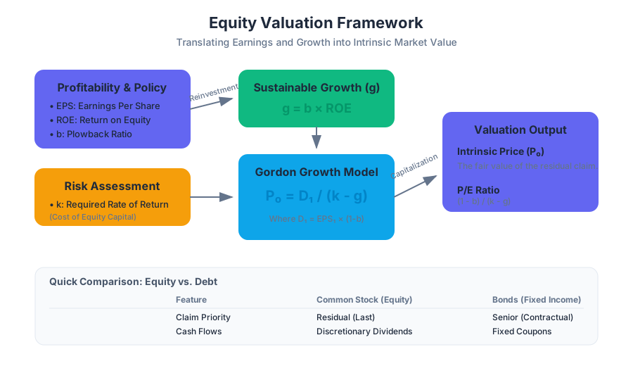
$$P_0 = \frac{D_1}{k - g}$$
2. Derivation (The Geometric Series Proof)
To understand why this works, consider the sum $S$: $$S = \frac{D_1}{1+k} + \frac{D_1(1+g)}{(1+k)^2} + \frac{D_1(1+g)^2}{(1+k)^3} + \dots$$
This is a geometric series with the first term $a = \frac{D_1}{1+k}$ and common ratio $r = \frac{1+g}{1+k}$. The sum of an infinite geometric series $a / (1-r)$ converges if $|r| < 1$ (which implies $k > g$).
$$P_0 = \frac{\frac{D_1}{1+k}}{1 - \frac{1+g}{1+k}} = \frac{D_1}{(1+k) - (1+g)} = \frac{D_1}{k - g}$$
3. Concrete Example
Suppose "BlueChip Corp" just paid a dividend ($D_0$) of $2.00. The expected growth rate ($g$) is 5%, and the required return ($k$) is 10%.
- Calculate $D_1$: $\text{\textdollar}2.00 \times (1 + 0.05) = \text{\textdollar}2.10$.
- Apply GGM: $P_0 = \frac{2.10}{0.10 - 0.05} = \frac{2.10}{0.05} = \text{\textdollar}42.00$.
4. Sensitivity Analysis
The GGM is highly sensitive to the inputs $k$ and $g$. As $g$ approaches $k$, the price approaches infinity.
| Growth Rate ($g$) | Required Return ($k$) | Resulting Price ($P_0$) |
|---|---|---|
| 4% | 10% | $35.00 |
| 5% | 10% | $42.00 |
| 6% | 10% | $53.00 |
| 5% | 9% | $52.50 |
5. Common Pitfalls
- $g \ge k$: If the growth rate exceeds the discount rate, the formula breaks down. In reality, no company can grow faster than the overall economy forever.
- Non-dividend payers: The GGM cannot directly value firms like Amazon or Google that reinvest all earnings (though one can argue $D_t$ represents the capacity to pay dividends).
Earnings-Per-Share (EPS) and the P/E Ratio
While dividends are the cash actually received by shareholders, Earnings-Per-Share (EPS) represents the total profit available to be either distributed or reinvested. The Price-Earnings (P/E) Ratio is the most widely used metric for relative valuation.
1. Definitions
- EPS: $\frac{\text{Total Net Income}}{\text{Shares Outstanding}}$
- Plowback Ratio ($b$): The fraction of earnings reinvested in the firm.
- Dividend Payout Ratio ($1-b$): The fraction of earnings paid out as dividends.
Therefore: $D_1 = EPS_1 \times (1-b)$.
2. The Link Between Growth and Reinvestment
A firm's growth rate is not arbitrary; it is a function of how much it reinvests and the return it earns on that reinvestment. $$g = \text{Retention Ratio} \times \text{Return on Equity (ROE)} = b \times ROE$$
3. Deriving the P/E Ratio
Starting from the GGM: $$P_0 = \frac{EPS_1(1-b)}{k - (b \times ROE)}$$
Dividing both sides by $EPS_1$: $$\frac{P_0}{EPS_1} = \frac{1-b}{k - g}$$
4. Determinants of the P/E Ratio
The P/E ratio is a reflection of three things:
- Growth opportunities: Higher $g$ leads to higher P/E.
- Risk: Higher $k$ (risk) leads to lower P/E.
- Accounting Quality: The "E" must represent true economic reality.
AI_DEMOI_DEMO--
Present Value of Growth Opportunities (PVGO)
One of the most powerful concepts in finance is the decomposition of a stock's price into two components: the value of its current assets and the value of its future growth.
1. What it is
The PVGO is the net present value of all future investments the firm will make. We can express the stock price as: $$P_0 = \frac{EPS_1}{k} + PVGO$$
Where:
- $\frac{EPS_1}{k}$: The value of the firm if it paid out all earnings as dividends (a "no-growth" firm).
- $PVGO$: The additional value created by reinvesting earnings into projects with $ROE > k$.
2. Why it matters: Growth vs. Value
A company can grow its earnings simply by reinvesting cash ($b > 0$), but this only adds value to the stock price if the return on those investments ($ROE$) exceeds the cost of capital ($k$).
- If $ROE > k$, then $PVGO > 0$ (Growth adds value).
- If $ROE = k$, then $PVGO = 0$ (Growth is value-neutral).
- If $ROE < k$, then $PVGO < 0$ (Growth destroys value).
3. Worked Example: The Growth Trap
Consider two firms, both with $EPS_1 = \text{\textdollar}5.00$ and $k = 10%$.
Firm A (High ROE): $b = 0.6$, $ROE = 15%$.
- $g = 0.6 \times 0.15 = 9%$.
- $P_0 = \frac{5(1-0.6)}{0.10 - 0.09} = \frac{2}{0.01} = \text{\textdollar}200$.
- No-growth value = $5 / 0.10 = \text{\textdollar}50$.
- $PVGO = \text{\textdollar}200 - \text{\textdollar}50 = \text{\textdollar}150$. (75% of value is growth).
Firm B (Low ROE): $b = 0.6$, $ROE = 8%$.
- $g = 0.6 \times 0.08 = 4.8%$.
- $P_0 = \frac{5(1-0.6)}{0.10 - 0.048} = \frac{2}{0.052} \approx \text{\textdollar}38.46$.
- No-growth value = $\text{\textdollar}50$.
- $PVGO = \text{\textdollar}38.46 - \text{\textdollar}50 = -\text{\textdollar}11.54$. (The firm is destroying value by reinvesting).
4. Summary Table: PVGO Dynamics
| Scenario | Condition | Impact of Increasing Plowback ($b$) | Stock Category |
|---|---|---|---|
| Value Creation | $ROE > k$ | Price Increases | Growth Stock |
| Value Neutral | $ROE = k$ | Price Unchanged | Mature/Income Stock |
| Value Destruction | $ROE < k$ | Price Decreases | "Empire Builders" |
Implementation: Multistage Valuation in Python
In the real world, companies often go through a "high growth" phase before maturing. A simple GGM is insufficient. We use a Two-Stage DDM where we discount individual dividends for the high-growth period and use a terminal value for the steady-state period.
def calculate_intrinsic_value(d0, high_g, stable_g, k, years_high_growth):
    """
    Calculates the intrinsic value of a stock using a two-stage DDM.

    d0: Current dividend
    high_g: Growth rate during high-growth phase (decimal)
    stable_g: Terminal growth rate (decimal)
    k: Required rate of return (decimal)
    years_high_growth: Duration of the first stage
    """
    pv_dividends = 0
    current_d = d0

    # Stage 1: High Growth Phase
    for t in range(1, years_high_growth + 1):
        current_d *= (1 + high_g)
        pv_dividends += current_d / ((1 + k) ** t)

    # Stage 2: Terminal Value (at the end of Stage 1)
    d_terminal = current_d * (1 + stable_g)
    terminal_price = d_terminal / (k - stable_g)
    pv_terminal_value = terminal_price / ((1 + k) ** years_high_growth)

    intrinsic_value = pv_dividends + pv_terminal_value
    return round(intrinsic_value, 2)

# Example: Tech startup transitioning to maturity
# $1.00 dividend, 20% growth for 5 years, then 4% stable growth. 10% discount rate.
price = calculate_intrinsic_value(1.00, 0.20, 0.04, 0.10, 5)
print(f"The intrinsic value is: ${price}")
# Output: The intrinsic value is: $34.58
Variations and Extensions
1. The H-Model
The H-model is a variation of the two-stage DDM that assumes the growth rate does not drop abruptly but rather declines linearly from a high initial rate to a stable terminal rate. This is often more realistic for firms facing increasing competition.
2. Free Cash Flow to Equity (FCFE)
For firms that do not pay dividends, analysts often substitute "Dividends" with FCFE, which is the cash flow available to be paid out after all reinvestment needs and debt obligations are met. $$FCFE = \text{Net Income} + \text{Depreciation} - \text{CapEx} - \Delta\text{Working Capital} + \text{Net Borrowing}$$
3. The Fed Model
The Fed Model compares the earnings yield ($E/P$) of the S&P 500 to the yield on 10-year Treasury bonds. While popular, it is often criticized for comparing a real variable (earnings, which grow with inflation) to a nominal variable (bond yields).
Common Pitfalls in Equity Valuation
- Double Counting Growth: Beginners often include growth in the cash flow projections and use a high P/E ratio for the terminal value. The terminal P/E should reflect a mature, stable-growth company.
- Ignoring Risk in $k$: Using a single discount rate for all companies. A biotech startup requires a significantly higher $k$ than a utility company due to the variance of its cash flows.
- The "Low P/E" Trap: Assuming a low P/E stock is "cheap." A low P/E might be a rational market response to a company with $ROE < k$ or a business model facing obsolescence.
- Terminal Value Dominance: In many DCF models, the terminal value accounts for 70-90% of the total price. Small changes in the terminal growth rate ($g$) can lead to massive swings in valuation, making the model appear more precise than it actually is.
Risk, Return, and Portfolio Theory
Key concepts: Mean-Variance Analysis · Standard Deviation and Correlation · Diversification · Sharpe Ratio · Tangency Portfolio
Introduction to the statistical relationship between risk and reward and the mathematical foundations of diversification.
Risk, Return, and Portfolio Theory
The transition from valuing individual assets—such as discounted cash flow analysis for equities or yield calculations for bonds—to Modern Portfolio Theory (MPT) represents a fundamental shift in financial economics. In the traditional view, an investment was judged solely on its own merits. However, since Harry Markowitz’s seminal work in 1952, we recognize that the risk of an individual asset is secondary to how that asset contributes to the risk of a collective portfolio.
This section explores the mechanics of risk and return, the mathematical elegance of diversification, and the identification of the "optimal" portfolio through Mean-Variance Analysis. We move beyond simple averages to understand the covariance of assets, ultimately deriving the Efficient Frontier and the Tangency Portfolio.
[AI_INFOGRAPHIC: A visual flow showing the progression from Individual Asset Statistics (Mean, Variance) -> The Covariance Matrix -> The Efficient Frontier construction -> The introduction of a Risk-Free Asset -> The Tangency Portfolio (Maximum Sharpe Ratio).]
Mean-Variance Analysis
Mean-Variance Analysis is the process of weighing the expected return of a portfolio against its realized volatility. In this framework, we assume investors are "risk-averse," meaning that for a given level of return, they prefer less risk, and for a given level of risk, they require a higher return.
The Mathematical Framework
We define the performance of an asset $i$ using two primary statistics:
- Expected Return ($E[R_i]$): The weighted average of all possible returns.
- Variance ($\sigma_i^2$): The measure of dispersion around the mean, representing risk.
For a portfolio $p$ consisting of $n$ assets with weights $w_i$, the portfolio's expected return is a simple linear combination:
$$E[R_p] = \sum_{i=1}^{n} w_i E[R_i]$$
However, the portfolio variance is not a simple linear combination of individual variances. It must account for how the assets move together:
$$\sigma_p^2 = \sum_{i=1}^{n} \sum_{j=1}^{n} w_i w_j \sigma_{ij}$$
where $\sigma_{ij}$ is the covariance between asset $i$ and asset $j$.
Why It Matters
Mean-Variance Analysis provides a quantitative "admissibility" criterion. An investment is considered mean-variance efficient if no other investment offers a higher return for the same risk, or lower risk for the same return. This allows us to discard sub-optimal portfolios and focus on the Efficient Frontier.
| Metric | Symbol | Description | Formula |
|---|---|---|---|
| Expected Return | $\mu$ or $E[R]$ | The "reward" component; the mean of the distribution. | $\sum p_i R_i$ |
| Standard Deviation | $\sigma$ | The "risk" component; the square root of variance. | $\sqrt{E[(R - E[R])^2]}$ |
| Weight | $w_i$ | The fraction of total capital allocated to asset $i$. | $Value_i / Value_{Total}$ |
| Covariance | $\sigma_{ij}$ | How two assets move in relation to each other. | $\rho_{ij} \sigma_i \sigma_j$ |
Standard Deviation and Correlation
The "magic" of portfolio theory lies in the fact that while portfolio return is the weighted average of individual returns, portfolio standard deviation is generally less than the weighted average of individual standard deviations. This phenomenon is driven by correlation.
The Correlation Coefficient ($\rho$)
Correlation is a dimensionless measure of the linear relationship between two variables, bounded by $-1$ and $+1$.
- $\rho = +1.0$: Perfect positive correlation. No risk reduction from diversification.
- $\rho = 0$: No linear relationship. Significant risk reduction.
- $\rho = -1.0$: Perfect negative correlation. Risk can be completely eliminated.
Derivation: The Two-Asset Case
To see the impact of correlation, consider a portfolio of two assets, A and B:
$$\sigma_p = \sqrt{w_A^2 \sigma_A^2 + w_B^2 \sigma_B^2 + 2 w_A w_B \sigma_A \sigma_B \rho_{AB}}$$
If $\rho_{AB} < 1$, the term $2 w_A w_B \sigma_A \sigma_B \rho_{AB}$ is smaller than it would be if the assets were perfectly correlated. Consequently, $\sigma_p < w_A \sigma_A + w_B \sigma_B$.
Concrete Example: The Power of Low Correlation
Assume two stocks, both with an expected return of 10% and a standard deviation of 20%.
| Correlation ($\rho$) | Portfolio Weight (A/B) | Portfolio Return | Portfolio Std Dev ($\sigma_p$) |
|---|---|---|---|
| +1.0 | 50% / 50% | 10% | 20.0% |
| +0.5 | 50% / 50% | 10% | 17.3% |
| 0.0 | 50% / 50% | 10% | 14.1% |
| -0.5 | 50% / 50% | 10% | 10.0% |
| -1.0 | 50% / 50% | 10% | 0.0% |
Key Insight: You can maintain the same 10% return while slashing your risk from 20% to 14.1% simply by finding two assets that are uncorrelated ($\rho=0$).
[AI_DEMO: An interactive scatter plot where users can adjust the correlation slider between two assets and watch the "bend" of the portfolio opportunity set change. At $\rho=1$, it's a straight line; as $\rho$ decreases, the line bows toward the Y-axis (lower risk).]
Diversification
Diversification is often called the "only free lunch in finance." It is the practical application of the mathematical principle that covariance matters more than individual variance in a large portfolio.
Systematic vs. Idiosyncratic Risk
As we add more assets to a portfolio, the contribution of each individual asset's variance ($\sigma_i^2$) begins to vanish, while the average covariance between assets ($\sigma_{ij}$) remains.
- Idiosyncratic Risk (Unsystematic/Specific): Risk unique to a specific company (e.g., a CEO scandal or a factory fire). This can be diversified away.
- Systematic Risk (Market): Risk that affects the entire economy (e.g., interest rate changes, recessions). This cannot be diversified away.
The $1/N$ Portfolio Limit
In an equally weighted portfolio ($w_i = 1/N$), the variance is: $$\sigma_p^2 = \frac{1}{N} (\text{Average Variance}) + \left(1 - \frac{1}{N}\right) (\text{Average Covariance})$$
As $N \to \infty$, the first term goes to zero. The risk of a well-diversified portfolio is determined solely by the average covariance of the stocks within it.
Common Pitfalls
- The Correlation Breakdown: In times of extreme market stress (e.g., the 2008 financial crisis), correlations often "spike to one." Assets that appeared uncorrelated suddenly move in lockstep, causing diversification to fail exactly when it is needed most.
- Over-diversification: Adding hundreds of assets can lead to "closet indexing," where the investor pays active management fees for a portfolio that merely mimics the market index.
The Sharpe Ratio
Once we have constructed the Efficient Frontier (the set of portfolios offering the highest return for each level of risk), we need a way to select the "best" one. William Sharpe introduced the Sharpe Ratio to measure the excess return per unit of risk.
Definition
The Sharpe Ratio ($S$) is defined as: $$S = \frac{E[R_p] - R_f}{\sigma_p}$$ where $R_f$ is the risk-free rate (typically the yield on a 3-month Treasury bill).
Why It Matters
The Sharpe Ratio represents the slope of the Capital Allocation Line (CAL). The CAL is the line representing all possible combinations of the risk-free asset and a specific risky portfolio. A higher Sharpe Ratio means a steeper CAL, providing a better trade-off between risk and reward.
| Sharpe Ratio Range | Interpretation |
|---|---|
| < 1.0 | Sub-optimal; the risk taken is not well-compensated by excess return. |
| 1.0 - 1.9 | Good; standard for many diversified equity funds. |
| 2.0 - 2.9 | Very Good; indicative of high-performing hedge funds or strategies. |
| 3.0+ | Excellent; often unsustainable in the long run due to capacity constraints. |
The Tangency Portfolio
The Tangency Portfolio is the unique point on the Efficient Frontier where the Sharpe Ratio is maximized. It is the point where the Capital Allocation Line (CAL) is exactly tangent to the Efficient Frontier.
How It Works: The Two-Step Optimization
- Identify the Tangency Portfolio: Find the weights $w_i$ that maximize the Sharpe Ratio. This portfolio is purely "risky" (contains no risk-free asset).
- The Separation Theorem: Regardless of an investor's risk aversion, they should all hold the same risky portfolio (the Tangency Portfolio). They only differ in how they split their total wealth between this Tangency Portfolio and the risk-free asset.
- Conservative Investors: Put 80% in $R_f$ and 20% in the Tangency Portfolio.
- Aggressive Investors: Borrow at $R_f$ (leverage) to put 150% in the Tangency Portfolio.
Implementation: Matrix Notation
In practice, calculating the Tangency Portfolio for $N$ assets requires solving a quadratic programming problem. Using matrix notation, where $\mathbf{\mu}$ is the vector of excess returns and $\mathbf{\Sigma}$ is the covariance matrix, the optimal weights $\mathbf{w^}$ are proportional to: $$\mathbf{w^} \propto \mathbf{\Sigma}^{-1} \mathbf{\mu}$$
Implementation Example (Python)
The following code demonstrates how to calculate the portfolio return and volatility for a set of assets using NumPy.
import numpy as np

def portfolio_metrics(weights, returns, cov_matrix, rf_rate=0.02):
    """
    Calculates Expected Return, Volatility, and Sharpe Ratio.
    """
    # Ensure weights sum to 1
    weights = weights / np.sum(weights)

    # Expected Portfolio Return
    p_ret = np.sum(returns * weights)

    # Portfolio Volatility (Standard Deviation)
    # Formula: sqrt( w.T * Sigma * w )
    p_vol = np.sqrt(np.dot(weights.T, np.dot(cov_matrix, weights)))

    # Sharpe Ratio
    sharpe = (p_ret - rf_rate) / p_vol

    return p_ret, p_vol, sharpe

# Example Data: 3 Assets
returns = np.array([0.12, 0.15, 0.08])
cov_matrix = np.array([
    [0.04, 0.02, 0.01],
    [0.02, 0.09, 0.03],
    [0.01, 0.03, 0.02]
])
weights = np.array([0.4, 0.4, 0.2])

res_ret, res_vol, res_sharpe = portfolio_metrics(weights, returns, cov_matrix)
print(f"Return: {res_ret:.2%}, Vol: {res_vol:.2%}, Sharpe: {res_sharpe:.2f}")
Extensions and Variations
While the standard Mean-Variance framework is the bedrock of finance, several extensions address its real-world limitations:
- Black-Litterman Model: Combines market equilibrium with investor views to create more stable weight estimates, preventing the "extreme weights" often produced by raw Mean-Variance optimization.
- The Resampled Efficient Frontier: Uses Monte Carlo simulations to account for estimation error in expected returns and covariances.
- Post-Modern Portfolio Theory (PMPT): Replaces standard deviation (which penalizes upside volatility) with Downside Deviation (Sortino Ratio), focusing only on "bad" risk.
- Multi-Factor Models (APT): Expands the definition of risk beyond the market index to include factors like Size, Value, and Momentum.
- Mean-Variance Analysis: The framework of optimizing the trade-off between expected return and variance.
- Efficient Frontier: The set of portfolios that offer the maximum return for a given level of risk.
- Systematic Risk: Non-diversifiable market risk (e.g., inflation, GDP growth).
- Idiosyncratic Risk: Firm-specific risk that can be eliminated via diversification.
- Tangency Portfolio: The portfolio on the efficient frontier with the highest Sharpe Ratio.
- Capital Allocation Line (CAL): The line representing combinations of the risk-free asset and a risky portfolio.
- Separation Theorem: The idea that the choice of risky portfolio is independent of an individual's risk preference.
- If two assets have a correlation of -1.0, is it possible to create a portfolio with zero risk? (Yes, by weighting them inversely to their standard deviations).
- Why does the Sharpe Ratio use excess return (Return - Risk-free rate) instead of just total return? (To measure the compensation received specifically for taking on risk above the guaranteed rate).
- As the number of assets in a portfolio increases, which component of variance becomes dominant: individual asset variance or average covariance? (Average covariance).
- True or False: An investor with high risk aversion will choose a different Tangency Portfolio than an investor with low risk aversion. (False; they choose the same Tangency Portfolio but different allocations to the risk-free asset).
Lecture Summary: Risk, Return, and Portfolio Theory
- Core Objective: Transition from individual asset selection to optimal portfolio construction.
- Key Formulae to Memorize:
- Portfolio Return: $E[R_p] = \sum w_i E[R_i]$
- Portfolio Variance (2-asset): $\sigma_p^2 = w_A^2\sigma_A^2 + w_B^2\sigma_B^2 + 2w_Aw_B\sigma_A\sigma_B\rho_{AB}$
- Sharpe Ratio: $(E[R_p] - R_f) / \sigma_p$
- Critical Concepts:
- The "Free Lunch": Diversification reduces risk without necessarily reducing return, provided $\rho < 1$.
- The Efficient Frontier: The upper boundary of the feasible set of portfolios.
- The Tangency Portfolio: The optimal risky portfolio for all investors.
- Real-World Application: Use Mean-Variance Analysis to determine asset allocation (e.g., 60% Stocks / 40% Bonds), but be wary of correlation spikes during market crashes.
Asset Pricing Models: CAPM and APT
Key concepts: Capital Asset Pricing Model (CAPM) · Beta (β) · Security Market Line (SML) · Arbitrage Pricing Theory (APT) · Systematic vs. Idiosyncratic Risk
Examination of equilibrium models that determine the required rate of return for risky assets.
Asset Pricing Models: CAPM and APT
In the trajectory of modern finance, the transition from Markowitz’s Portfolio Selection—which focuses on how an individual should invest—to Asset Pricing Models represents a shift from normative behavior to positive equilibrium. If Portfolio Theory tells us how to construct the "best" portfolio, Asset Pricing Models like the Capital Asset Pricing Model (CAPM) and Arbitrage Pricing Theory (APT) explain how the collective actions of all investors result in the prices and expected returns we observe in the marketplace.
These models serve as the foundational "hurdle rate" logic in corporate finance. Whether a CFO is deciding on a multi-billion dollar capital expenditure or a fund manager is evaluating a tech IPO, they are using the mathematical frameworks derived from CAPM and APT to determine if the expected return justifies the inherent risk.
AI_SVGI_SVG## The Fundamental Dichotomy: Systematic vs. Idiosyncratic Risk
Before deriving specific models, we must establish the two-part nature of risk. In a diversified economy, not all uncertainty is created equal.
- Systematic Risk (Market Risk): This refers to fluctuations that affect the entire market simultaneously. Examples include changes in GDP, interest rate hikes, or global pandemics. Because these factors impact all firms to varying degrees, this risk cannot be diversified away.
- Idiosyncratic Risk (Specific Risk): This refers to risks unique to a specific company or industry, such as a CEO resignation, a localized factory fire, or a successful patent application. In a large enough portfolio, these "shocks" cancel each other out.
The Diversification Principle: In a competitive market, investors are not compensated for bearing idiosyncratic risk. Because this risk can be eliminated for free (via diversification), the market price of idiosyncratic risk is zero. Only systematic risk commands a risk premium.
| Feature | Systematic Risk | Idiosyncratic Risk |
|---|---|---|
| Synonyms | Market Risk, Undiversifiable Risk | Firm-Specific Risk, Unique Risk |
| Source | Macroeconomic factors (Inflation, GDP) | Microeconomic factors (Strikes, R&D) |
| Remedy | Hedging / Asset Allocation | Diversification |
| Market Reward | Yes (Risk Premium) | No |
The Capital Asset Pricing Model (CAPM)
Developed independently by Sharpe (1964), Lintner (1965), and Mossin (1966), the CAPM is a linear model that predicts the expected return of an asset based on its sensitivity to the broad market.
The Assumptions of CAPM
To arrive at the elegant simplicity of the CAPM, we assume a "frictionless" world:
- Rationality: Investors are mean-variance optimizers.
- Homogeneous Expectations: All investors have the same estimates of expected returns, variances, and covariances.
- Single-Period Horizon: All investors plan for the same time duration.
- Perfect Markets: No taxes, no transaction costs, and assets are infinitely divisible.
- Risk-Free Rate: Investors can borrow and lend at the same risk-free rate ($R_f$).
The CAPM Formula
The expected return of any asset $i$ is defined as:
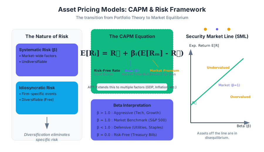
$$E[R_i] = R_f + \beta_i (E[R_m] - R_f)$$
Where:
- $E[R_i]$: Expected return on asset $i$.
- $R_f$: The risk-free rate (typically long-term government bond yields).
- $\beta_i$: The asset's Beta, measuring systematic risk.
- $E[R_m] - R_f$: The Equity Market Risk Premium (EMRP), the extra return required for moving from a risk-free asset to the risky market portfolio.
Beta (β): The Measure of Sensitivity
Beta is the most critical parameter in the CAPM. It represents the marginal contribution of an asset to the risk of the market portfolio. Mathematically, it is the ratio of the covariance between the asset and the market to the variance of the market:
$$\beta_i = \frac{Cov(R_i, R_m)}{Var(R_m)} = \rho_{im} \frac{\sigma_i}{\sigma_m}$$
Where $\rho_{im}$ is the correlation between the asset and the market.
Interpreting Beta Values
- $\beta = 1$: The asset moves in lockstep with the market. If the market rises 10%, the asset is expected to rise 10%.
- $\beta > 1$: "Aggressive" assets. These are more sensitive to market swings (e.g., high-growth tech stocks).
- $0 < \beta < 1$: "Defensive" assets. These move less than the market (e.g., utility companies).
- $\beta = 0$: The asset has no systematic risk (e.g., the risk-free asset).
- $\beta < 0$: The asset moves inversely to the market (extremely rare, sometimes seen in gold or specific hedging instruments).
| Asset Class | Typical Beta Range | Sensitivity Description |
|---|---|---|
| Treasury Bills | 0.0 | No market sensitivity |
| Utilities | 0.4 – 0.7 | Low sensitivity; "Defensive" |
| S&P 500 Index | 1.0 | The Market Benchmark |
| Tech / Biotech | 1.2 – 2.5 | High sensitivity; "Aggressive" |
The Security Market Line (SML)
The Security Market Line is the graphical representation of the CAPM. It plots the relationship between an asset's Beta (x-axis) and its Expected Return (y-axis).
In equilibrium, all assets should lie exactly on the SML.
- If an asset lies above the SML, it is undervalued (it offers too much return for its risk). Investors will buy it, driving the price up and the expected return down until it hits the SML.
- If an asset lies below the SML, it is overvalued. Investors will sell it, driving the price down and the expected return up until it hits the SML.
SML vs. CML (Capital Market Line)
A common point of confusion in Finance Theory I is the difference between the CML and the SML:
- CML: Relates the return of efficient portfolios to their total risk (Standard Deviation). It only applies to perfectly diversified portfolios.
- SML: Relates the return of any asset (efficient or not) to its systematic risk (Beta).
Implementation: Calculating Beta in Python
In practice, $\beta$ is estimated using a "Market Model" regression. We regress the excess returns of a stock against the excess returns of a market index (like the S&P 500).
import numpy as np
import pandas as pd
import statsmodels.api as sm

def calculate_beta(stock_returns, market_returns, rf_rate):
    """
    Calculates the Beta of a stock using OLS regression.
    Formula: (R_i - R_f) = alpha + beta * (R_m - R_f)
    """
    # Calculate excess returns
    y = stock_returns - rf_rate
    X = market_returns - rf_rate

    # Add a constant for the intercept (Alpha)
    X = sm.add_constant(X)

    # Fit the Ordinary Least Squares (OLS) model
    model = sm.OLS(y, X).fit()

    # Return the beta coefficient
    return model.params[1], model.rsquared

# Example Usage:
# stock_ret = pd.Series([...]) # Daily returns of AAPL
# mkt_ret = pd.Series([...])   # Daily returns of SPY
# beta, r_sq = calculate_beta(stock_ret, mkt_ret, 0.02/252)
# print(f"Beta: {beta:.2f}, R-Squared: {r_sq:.2f}")
AI_DEMOI_DEMO--
Arbitrage Pricing Theory (APT)
While the CAPM is elegant, it relies on the existence of a single "Market Portfolio" that is impossible to observe in reality (Roll’s Critique). Stephen Ross developed Arbitrage Pricing Theory (APT) in 1976 as an alternative that requires fewer assumptions.
The Core Logic: The Law of One Price
APT is built on the principle of no-arbitrage. It suggests that if two assets have the same exposure to risk factors, they must have the same expected return. If they didn't, an arbitrageur could buy the cheaper one and sell the more expensive one, earning a risk-free profit until prices align.
The Multi-Factor Model
Unlike CAPM, which uses only one factor (the market), APT allows for $n$ factors. The return of an asset is modeled as:
$$R_i = E[R_i] + \beta_{i1}F_1 + \beta_{i2}F_2 + ... + \beta_{in}F_n + \epsilon_i$$
Where:
- $E[R_i]$: The expected return.
- $F_j$: The surprise (innovation) in factor $j$.
- $\beta_{ij}$: The sensitivity of asset $i$ to factor $j$.
- $\epsilon_i$: The idiosyncratic error term.
The expected return in the APT framework is:
$$E[R_i] = R_f + \beta_{i1}\lambda_1 + \beta_{i2}\lambda_2 + ... + \beta_{in}\lambda_n$$
Where $\lambda_j$ is the risk premium associated with factor $j$.
Common APT Factors
While APT doesn't specify what the factors are, empirical research (notably by Chen, Roll, and Ross) has identified several macro-variables that drive returns:
- Inflation: Unexpected changes in the CPI.
- GDP Growth: Unexpected changes in industrial production.
- Default Risk: Changes in the spread between high-yield and AAA bonds.
- Yield Curve: Shifts in the slope of the term structure of interest rates.
| Feature | CAPM | APT |
|---|---|---|
| Number of Factors | Exactly One (The Market) | Multiple (Macroeconomic) |
| Assumptions | High (Utility, Normal Distribution) | Low (No Arbitrage) |
| Market Portfolio | Required (Must be observable) | Not Required |
| Practicality | Easy to calculate, hard to prove | Hard to calculate, theoretically robust |
Practical Applications and Pitfalls
1. Calculating the Cost of Equity
The most common use of CAPM is determining the Cost of Equity ($K_e$) for the Weighted Average Cost of Capital (WACC).
- Example: A project has a Beta of 1.2. The risk-free rate is 3% and the market risk premium is 5%.
- $K_e = 3% + 1.2(5%) = 9%$.
- If the project's internal rate of return (IRR) is less than 9%, the firm should reject it.
2. Performance Evaluation (Alpha)
Investment managers are often judged by Jensen's Alpha ($\alpha$), which is the excess return of a portfolio over what CAPM predicts: $$\alpha_p = R_p - [R_f + \beta_p(R_m - R_f)]$$ A positive alpha suggests the manager has "beaten the market" through superior stock selection or timing.
3. Common Pitfalls
- Beta Instability: Beta is not a physical constant. A company's beta changes as it takes on more debt (levering up) or as its industry matures.
- The Proxy Problem: Most people use the S&P 500 as a proxy for the "Market Portfolio." However, the true market portfolio includes real estate, human capital, and private equity. If the proxy is wrong, the Beta is wrong.
- The "Beta is Dead" Debate: Fama and French (1992) famously showed that Beta has had a weak relationship with actual returns over long periods. They proposed the Fama-French Three-Factor Model, which adds Size (SMB) and Value (HML) factors to the CAPM.
Summary of Key Formulae
| Concept | Formula |
|---|---|
| CAPM Expected Return | $E[R_i] = R_f + \beta_i(E[R_m] - R_f)$ |
| Beta (Covariance) | $\beta_i = \frac{\sigma_{im}}{\sigma^2_m}$ |
| Jensen's Alpha | $\alpha = R_{actual} - R_{CAPM}$ |
| APT Expected Return | $E[R_i] = R_f + \sum \beta_{ij}\lambda_j$ |
| Sharpe Ratio | $S = \frac{E[R_p] - R_f}{\sigma_p}$ |
AI_STUDY_GUIDEI_STUDY_GUIDE### Core Definitions for Review
- Market Portfolio: A theoretical portfolio containing every risky asset in the world, weighted by market value. In CAPM, this is the only risky portfolio any investor needs to hold (combined with the risk-free asset).
- Separation Theorem: The idea that the investment decision (which risky assets to hold) is separate from the financing decision (how much risk to take by mixing with the risk-free asset).
- Risk Premium: The return in excess of the risk-free rate of return an investment is expected to yield; an asset's risk premium is a form of compensation for investors who tolerate the extra risk.
- Factor Loading: In APT, the $\beta_{ij}$ coefficient that represents how sensitive an asset is to a specific factor.
Final Thought for Finance Theory I
The transition from CAPM to APT reflects the evolution of financial thought from a single-factor, equilibrium-based world to a multi-factor, arbitrage-free world. While CAPM remains the standard for teaching and basic corporate valuation due to its intuitive appeal, APT and its descendants (like the Fama-French models) provide the empirical rigor required for modern institutional asset management.
Capital Budgeting and Corporate Investment
Key concepts: Incremental After-Tax Cash Flows · Internal Rate of Return (IRR) · Profitability Index · Depreciation Tax Shield · Project Beta
Practical application of valuation techniques to corporate decision-making and project evaluation.
Capital Budgeting and Corporate Investment
Capital budgeting is the strategic process by which a corporation determines which long-term investments or projects are worth pursuing. In the context of Finance Theory I, this represents the "Investment Decision"—the most critical driver of firm value. While the firm's financing decision determines how to pay for assets, the investment decision determines which assets to acquire in the first place.
The fundamental objective of capital budgeting is to identify projects that generate a return greater than the cost of the capital required to fund them. Mathematically, this is expressed through the maximization of Net Present Value (NPV). However, the transition from theoretical formulas to real-world application requires a rigorous understanding of cash flow estimation, tax implications, and risk adjustment.
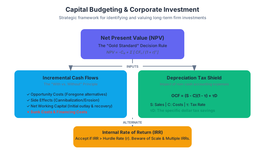
AI_SVGI_SVG## The Net Present Value (NPV) Framework
The Net Present Value (NPV) rule is the "gold standard" of capital budgeting. It states that a firm should accept all projects with a positive NPV and reject those with a negative NPV. If two projects are mutually exclusive, the firm should choose the one with the highest positive NPV.
Mathematical Definition
The NPV of a project is the sum of the present values of all its expected incremental cash flows, discounted at the appropriate risk-adjusted rate:
$$NPV = -C_0 + \sum_{t=1}^{T} \frac{CF_t}{(1 + r)^t}$$
Where:
- $C_0$ is the initial investment (outlay).
- $CF_t$ is the incremental after-tax cash flow at time $t$.
- $r$ is the discount rate (the opportunity cost of capital).
- $T$ is the project's life.
Why It Matters
NPV directly measures the expected increase in shareholder wealth. Unlike accounting metrics, NPV accounts for the Time Value of Money (TVM) and the specific risk profile of the project's cash flows. By discounting future dollars, we acknowledge that a dollar today is worth more than a dollar tomorrow, and a risky dollar is worth less than a certain one.
Incremental After-Tax Cash Flows
The most common error in capital budgeting is confusing accounting earnings with cash flows. For valuation purposes, only cash matters. Furthermore, we only care about incremental cash flows—the changes in the firm’s total cash flow that occur as a direct consequence of accepting the project.
The "With vs. Without" Principle
To identify incremental cash flows, ask: "What will the firm's total cash flows be with this project, minus what they would have been without it?"
| Feature | Include in NPV? | Reasoning |
|---|---|---|
| Sunk Costs | No | Costs already incurred (e.g., R&D, pilot studies) cannot be recovered and do not change regardless of the decision. |
| Opportunity Costs | Yes | If a project uses an existing asset (like land), the cash that asset could have generated elsewhere must be treated as a cost. |
| Side Effects | Yes | "Cannibalization" (new product reducing sales of an old one) or "Erosion" must be subtracted from the project's inflows. |
| Taxes | Yes | We only care about the cash available to distribute to investors; the government’s share is a real cash outflow. |
| Financing Costs | No | Interest and dividends are handled by the discount rate ($r$), not the cash flows. Including them in $CF_t$ would double-count the cost of capital. |
Net Working Capital (NWC)
Projects often require an initial investment in Net Working Capital (e.g., increasing inventory or accounts receivable). While these are not "expenses" in an accounting sense, they represent cash tied up in the business.
- Initial Outlay: An increase in NWC is a cash outflow.
- Project End: Usually, NWC is recovered at the end of the project's life, resulting in a final-year cash inflow.
The Depreciation Tax Shield
Depreciation is a non-cash accounting expense. You do not write a check to "Depreciation" every year. However, depreciation is tax-deductible. By reducing taxable income, depreciation reduces the actual cash paid in taxes. This effect is known as the Depreciation Tax Shield.
Derivation of After-Tax Cash Flow
Let $S$ be Sales, $C$ be Operating Costs, $D$ be Depreciation, and $\tau$ be the corporate tax rate.
- Accounting Profit (EBIT): $EBIT = S - C - D$
- Taxes Paid: $Taxes = (S - C - D) \times \tau$
- Net Income: $NI = (S - C - D) \times (1 - \tau)$
- Operating Cash Flow (OCF): $OCF = NI + D$ (Add back the non-cash expense)
By substituting (3) into (4), we get: $$OCF = (S - C - D)(1 - \tau) + D$$ $$OCF = (S - C)(1 - \tau) - D(1 - \tau) + D$$ $$OCF = (S - C)(1 - \tau) + \tau D$$
The Insight: The term $\tau D$ is the Depreciation Tax Shield. It represents the specific dollar amount saved in taxes due to the depreciation deduction.
Example: Calculating OCF
A project generates $100,000 in revenue and $40,000 in costs. Depreciation is $20,000. The tax rate is 21%.
- Method 1 (Bottom-Up): $NI = (100k - 40k - 20k) \times (1 - 0.21) = 31.6k$. $OCF = 31.6k + 20k = 51.6k$.
- Method 2 (Tax Shield): $OCF = (100k - 40k)(0.79) + (0.21 \times 20k) = 47.4k + 4.2k = 51.6k$.
Internal Rate of Return (IRR)
The Internal Rate of Return (IRR) is the discount rate that makes the NPV of a project equal to zero. It represents the project's expected percentage rate of return.
The Decision Rule
- Accept if $IRR > r$ (where $r$ is the hurdle rate/cost of capital).
- Reject if $IRR < r$.
Pitfalls of IRR
While intuitively appealing to managers, IRR has several mathematical flaws that make it secondary to NPV:
- Multiple IRRs: If a project has "non-conventional" cash flows (where the sign changes more than once, e.g., - + -), there may be multiple solutions for $IRR$. This is a result of Descartes' Rule of Signs for polynomials.
- The Scale Problem: IRR ignores the absolute dollar value. A 100% return on $1 is worse than a 10% return on $1,000,000, but IRR would rank the former higher.
- Reinvestment Assumption: IRR implicitly assumes that intermediate cash flows are reinvested at the IRR itself. NPV assumes they are reinvested at the more realistic cost of capital ($r$).
| Metric | Strengths | Weaknesses |
|---|---|---|
| NPV | Theoretically sound; accounts for scale; additive. | Harder to communicate to non-financial managers. |
| IRR | Expressed as a percentage (intuitive); easy to compare to interest rates. | Multiple solutions; scale neglect; reinvestment bias. |
AI_DEMOI_DEMO--
Profitability Index (PI)
The Profitability Index is the ratio of the present value of future cash flows to the initial investment.
$$PI = \frac{PV(\text{Future Cash Flows})}{\text{Initial Investment}} = \frac{NPV + |C_0|}{|C_0|}$$
Application: Capital Rationing
PI is particularly useful when a firm faces Capital Rationing—a limit on the total budget available for new investments. In this scenario, the goal is not just to find positive NPV projects, but to find the "biggest bang for the buck."
- Rule: Rank projects by PI and accept them in descending order until the budget is exhausted.
Project Beta and the Risk-Adjusted Discount Rate
A common mistake is using the firm's overall Weighted Average Cost of Capital (WACC) to discount all projects. However, the discount rate should reflect the risk of the project, not the risk of the firm.
If a software company (low risk) decides to invest in a gold mine (high risk), using the software WACC would lead to an overvaluation of the gold mine. We must find a Project Beta.
The "Pure Play" Method
To find the appropriate beta for a project:
- Identify "Pure Play" companies that operate solely in the project's industry.
- Unlever their equity betas to find the Asset Beta ($\beta_A$), removing the effect of their specific leverage.
- Relever the average Asset Beta using the firm's own target debt-to-equity ratio to find the project's equity beta.
Unlevering Formula (Hamada Equation): $$\beta_A = \frac{\beta_E}{1 + (1 - \tau)(D/E)}$$
Implementation in Python
The following code demonstrates a simple NPV and IRR calculation using standard financial logic.
import numpy as np
import numpy_financial as npf

def evaluate_project(cash_flows, discount_rate):
    """
    Calculates NPV, IRR, and PI for a given set of cash flows.
    cash_flows: list, where index 0 is the initial investment (negative)
    """
    npv = npf.npv(discount_rate, cash_flows)
    irr = npf.irr(cash_flows)

    # PI = PV of future flows / Initial Investment
    pv_future = npv - cash_flows[0]
    pi = pv_future / abs(cash_flows[0])

    return {
        "NPV": round(npv, 2),
        "IRR": f"{round(irr * 100, 2)}%",
        "PI": round(pi, 2)
    }

# Example: Project requiring $100k, returning $30k, $40k, $50k, $20k
project_cfs = [-100000, 30000, 40000, 50000, 20000]
r = 0.10 # 10% discount rate

results = evaluate_project(project_cfs, r)
print(f"Project Analysis: {results}")
# Output: Project Analysis: {'NPV': 13813.26, 'IRR': '16.54%', 'PI': 1.14}
Summary of Decision Rules
| Method | Decision Rule | Best Used When... |
|---|---|---|
| NPV | Accept if $> 0$ | Always. It is the most reliable metric. |
| IRR | Accept if $> r$ | Comparing projects of similar scale/timing. |
| PI | Accept if $> 1$ | Facing a constrained capital budget. |
| Payback | Accept if $< X$ years | Liquidity is the primary concern (ignores TVM). |
Common Pitfalls in Capital Budgeting
- Ignoring Inflation: If the discount rate is a nominal rate (which it usually is), the cash flow projections must also be nominal. Mixing real cash flows with nominal discount rates leads to significant undervaluation.
- Overestimating Terminal Value: Many projects assume a "perpetuity" value at the end. Small changes in the growth rate ($g$) or discount rate ($r$) in the Gordon Growth Model ($TV = \frac{CF_{T+1}}{r - g}$) can swing the NPV wildly.
- The "Pet Project" Bias: Managers may adjust cash flow estimates or discount rates to ensure their preferred project shows a positive NPV. This is why sensitivity analysis and scenario analysis are vital.
- Ignoring Real Options: NPV is a "now or never" calculation. In reality, managers have the option to expand, contract, or abandon projects based on new information. Traditional NPV often underestimates the value of projects with high flexibility.
Market Efficiency and Behavioral Finance
Key concepts: Efficient Markets Hypothesis (EMH) · Behavioral Finance · Adaptive Markets Hypothesis (AMH) · Market Anomalies · Psychology of Risk
A critical look at how information is processed by markets and the psychological factors that influence investor behavior.
Market Efficiency and Behavioral Finance
In the study of financial economics, the tension between market efficiency and human psychology represents one of the most profound intellectual divides. Traditional finance, rooted in the Efficient Markets Hypothesis (EMH), views market participants as rational "Expected Utility Maximizers" and prices as the unbiased reflection of all available information. Conversely, Behavioral Finance draws on psychology and sociology to argue that cognitive biases and emotional responses systematically distort market prices.
The modern synthesis, the Adaptive Markets Hypothesis (AMH), reconciles these views by applying the principles of evolutionary biology to financial interactions. This section explores the mechanics of these theories, the mathematical foundations of market efficiency, the psychological drivers of risk, and the empirical anomalies that continue to challenge our understanding of capital markets.
AI_SVGI_SVG## The Efficient Markets Hypothesis (EMH)
The Efficient Markets Hypothesis, formalized by Eugene Fama in 1970, asserts that financial markets are "informationally efficient." In such a market, the current price of a security is the best estimate of its intrinsic value, given the information available to the public.
1. Mathematical Foundation: The Martingale Property
At its core, the EMH implies that price changes (returns) should be unpredictable. If a price change were predictable, rational investors would trade on that information immediately, shifting the price until the advantage disappears. Mathematically, this is often expressed via the Martingale Property:
Definition: The Martingale Property A stochastic process ${P_t}$ is a martingale with respect to a sequence of information sets ${\Phi_t}$ if: $$E[P_{t+1} | \Phi_t] = P_t$$ In finance, we adjust this for the required rate of return $r$: $$E[P_{t+1} | \Phi_t] = P_t(1 + E[r])$$
This implies that the best predictor of tomorrow's price is today's price, adjusted for the expected return. Any deviation from this is "noise" or "news" ($ \epsilon_{t+1} $), which by definition is uncorrelated with past information: $$P_{t+1} = P_t(1 + E[r]) + \epsilon_{t+1}$$ where $E[\epsilon_{t+1} | \Phi_t] = 0$.
2. The Three Forms of Efficiency
Fama categorized market efficiency into three levels based on the composition of the information set $\Phi_t$:
| Form | Information Set ($\Phi_t$) | Implication |
|---|---|---|
| Weak-Form | Past prices and trading volume. | Technical analysis (charting) cannot produce alpha. |
| Semi-Strong Form | All publicly available information (earnings, news, macro data). | Fundamental analysis is already "priced in." |
| Strong-Form | All information, including private/insider information. | Even insiders cannot consistently achieve abnormal returns. |
3. The Joint Hypothesis Problem
A critical pitfall in testing the EMH is the Joint Hypothesis Problem. To determine if a market is efficient, you must use an asset pricing model (like the CAPM) to determine what the "correct" price should be. If you find an anomaly, you cannot know if the market is inefficient or if your pricing model is simply wrong.
Behavioral Finance: The Psychology of the Market
Behavioral Finance argues that because markets are populated by humans, they are subject to human frailty. It challenges the Homo Economicus model of perfect rationality.
1. Prospect Theory and Loss Aversion
Developed by Daniel Kahneman and Amos Tversky, Prospect Theory replaces the standard Utility Function with a Value Function.
- S-Shaped Curve: People are risk-averse regarding gains but risk-seeking regarding losses.
- Loss Aversion: The pain of losing $1,000 is psychologically twice as powerful as the joy of gaining $1,000.
2. Cognitive Biases and Heuristics
Investors use mental shortcuts (heuristics) that lead to systematic errors.
| Bias | Description | Market Impact |
|---|---|---|
| Overconfidence | Overestimating the precision of one's information. | Excessive trading volume and price volatility. |
| Anchoring | Over-relying on the first piece of information offered (e.g., purchase price). | Prices adjust too slowly to new information. |
| Representativeness | Assuming a small sample represents the whole (e.g., "hot hand" fallacy). | Overreaction to short-term performance (bubbles). |
| Conservatism | Being too slow to update beliefs in the face of new evidence. | Underreaction to earnings announcements. |
3. Limits to Arbitrage
If some investors are irrational, why don't rational "arbitrageurs" trade against them and push prices back to efficiency? Behavioral finance points to Limits to Arbitrage:
- Fundamental Risk: The "mispricing" might get worse before it gets better.
- Noise Trader Risk: Irrational traders may push prices even further from equilibrium, forcing arbitrageurs to liquidate positions due to margin calls.
- Implementation Costs: Commissions, bid-ask spreads, and short-sale constraints.
"The market can remain irrational longer than you can remain solvent." — John Maynard Keynes
Market Anomalies
Anomalies are empirical results that seem to contradict the EMH. They suggest that certain strategies can consistently earn "abnormal" returns (returns in excess of what is predicted by the CAPM).
1. The Size Effect (Small-Firm Effect)
Historically, small-cap stocks have outperformed large-cap stocks, even after adjusting for Beta. This suggests that the CAPM might be missing a "size risk" factor.
2. Value Premium
Stocks with low Price-to-Book (P/B) or Price-to-Earnings (P/E) ratios (Value stocks) tend to outperform stocks with high ratios (Growth stocks).
3. Momentum
The tendency for stocks that have performed well in the recent past (3–12 months) to continue performing well in the near future. This directly contradicts the Weak-Form EMH, as it implies that past prices can predict future returns.
4. Post-Earnings Announcement Drift (PEAD)
When a company releases surprisingly good earnings, the price doesn't jump to the new equilibrium immediately. Instead, it "drifts" upward for several weeks. This is a classic example of Underreaction.
AI_DEMOI_DEMO--
The Adaptive Markets Hypothesis (AMH)
Proposed by Professor Andrew Lo, the Adaptive Markets Hypothesis provides a framework to reconcile EMH with Behavioral Finance. Instead of viewing efficiency as an all-or-nothing state, AMH views it as a variable that changes over time based on the "ecology" of the market.
1. Core Principles of AMH
- Individuals are neither always rational nor always irrational; they are biological entities whose behavior is shaped by evolution.
- Individuals display biases and make sub-optimal decisions, but they learn and adapt.
- Competition, adaptation, and natural selection drive market dynamics.
- Market efficiency is not a law of nature but a product of the number of "species" (types of investors) and the resources (profit opportunities) available.
2. The Evolutionary Mechanism
In the AMH framework, investment strategies are like species. A strategy that works in a low-interest-rate environment (e.g., "Carry Trade") might go "extinct" when macro conditions change.
- Profit Opportunities: These are the "food" for investors.
- Competition: As more investors adopt a successful strategy, the "food" becomes scarce, and the market becomes more efficient.
- Innovation: When the environment changes, new strategies must evolve to survive.
3. Comparison of Frameworks
| Feature | EMH | Behavioral Finance | AMH |
|---|---|---|---|
| Market State | Always Efficient | Often Inefficient | Dynamic/Changing |
| Human Behavior | Rational | Biased/Irrational | Heuristic/Adaptive |
| Risk/Reward | Linear/Stable | Psychologically Distorted | Evolutionary/Contextual |
| Market Crashes | External Shocks | Pathological Failures | Evolutionary Adaptation |
Implementation: Simulating Market Dynamics
To understand the difference between a "Random Walk" (EMH) and a "Trending/Momentum" market (Anomaly), we can model price paths in Python.
import numpy as np
import matplotlib.pyplot as plt

def simulate_market(days=252, drift=0.0005, vol=0.01, momentum_factor=0.1):
    """
    Simulates two price paths:
    1. Pure Random Walk (EMH)
    2. Momentum-biased Walk (Behavioral/Anomaly)
    """
    # Initialize price arrays
    p_emh = np.zeros(days)
    p_mom = np.zeros(days)
    p_emh[0] = p_mom[0] = 100

    # Generate random shocks
    shocks = np.random.normal(drift, vol, days)

    for t in range(1, days):
        # EMH: Price depends only on the current shock
        p_emh[t] = p_emh[t-1] * (1 + shocks[t])

        # Momentum: Current return is influenced by the previous return
        prev_ret = (p_mom[t-1] - p_mom[t-2]) / p_mom[t-2] if t > 1 else 0
        p_mom[t] = p_mom[t-1] * (1 + shocks[t] + (momentum_factor * prev_ret))

    return p_emh, p_mom

# Visualization
emh_path, mom_path = simulate_market()
plt.figure(figsize=(10, 5))
plt.plot(emh_path, label='Efficient Market (Random Walk)')
plt.plot(mom_path, label='Momentum Market (Adaptive/Behavioral)')
plt.title("Market Efficiency vs. Momentum Anomaly")
plt.legend()
plt.show()
The Psychology of Risk
Risk is not just a mathematical standard deviation ($\sigma$); it is a physiological experience.
1. Neurofinance
Research shows that financial gains stimulate the same reward centers in the brain (the nucleus accumbens) as food or drugs. Conversely, financial losses or the threat of a crash activate the amygdala, the brain's fear center.
2. Risk vs. Uncertainty (Knightian Uncertainty)
- Risk: The outcomes are unknown, but the probability distribution is known (e.g., a roulette wheel).
- Uncertainty: The probability distribution itself is unknown (e.g., a geopolitical crisis).
Behavioral finance suggests that humans are "Ambiguity Averse"—we prefer a known risk over an unknown uncertainty, which often leads to "panic selling" during unprecedented events where probabilities cannot be calculated.
3. The Disposition Effect
This is the tendency for investors to sell winning stocks too early (to "lock in" a gain, satisfying the risk-averse part of the Prospect Theory curve) and hold losing stocks too long (to avoid "realizing" a loss, staying in the risk-seeking part of the curve).
Common Pitfalls in Market Analysis
- Confusing Luck with Skill: In a random walk, some "monkeys" will inevitably throw darts that hit the bullseye. This is the Survivor Bias.
- Data Mining: If you test enough variables against historical stock prices, you will find a "pattern" that worked in the past but has no predictive power for the future.
- Ignoring Transaction Costs: Many anomalies (like high-frequency momentum) disappear once you account for the costs of trading and taxes.
- Over-reliance on Beta: Assuming $\beta$ is the only measure of risk. The existence of the Size and Value premiums suggests that risk is multi-dimensional.
AI_QUIZI_STUDY_GUIDE--
AI Study Guide: Market Efficiency and Behavioral Finance
Key Formulas to Master
- Martingale Expectation: $E[P_{t+1} | \Phi_t] = P_t(1 + r)$
- Abnormal Return (Alpha): $\alpha_i = R_i - [R_f + \beta_i(R_m - R_f)]$
- Sharpe Ratio: $S = \frac{E[R_p - R_f]}{\sigma_p}$ (Used to evaluate if an anomaly provides better risk-adjusted returns).
Concept Checklist
- Can you explain why the "Joint Hypothesis Problem" makes it impossible to definitively prove market inefficiency?
- Do you understand the difference between "Weak-form" and "Semi-strong form" efficiency?
- Can you describe the S-shaped value function of Prospect Theory?
- How does the Adaptive Markets Hypothesis explain the disappearance of certain market anomalies over time?
- What is the "Disposition Effect" and how does it relate to loss aversion?
Summary of the "Great Debate"
- EMH (Fama): Prices are right; you can't beat the market; risk and return are linearly related.
- Behavioral (Thaler/Kahneman): Prices are wrong because people are biased; arbitrage is limited; psychology drives bubbles.
- AMH (Lo): Efficiency is an ecosystem; it fluctuates based on competition and environmental changes; "rationality" is an adaptive trait.
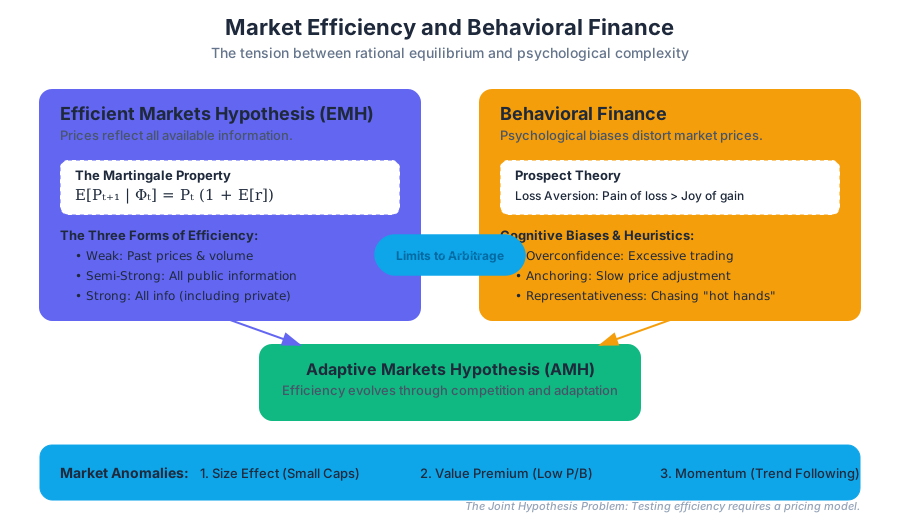
Introduction to Derivatives: Forwards, Futures, and Options
Key concepts: Forward and Futures Contracts · Call and Put Options · Payoff Diagrams · Binomial Model · Counterparty Risk
Introduction to derivative instruments, their payoff structures, and fundamental pricing models.
Introduction to Derivatives: Forwards, Futures, and Options
In the study of financial economics, derivatives represent a monumental shift from valuing assets based on their intrinsic cash flows to valuing contracts based on the behavior of an underlying reference price. As we transition from the Capital Asset Pricing Model (CAPM) and fixed-income valuation, we enter the realm of contingent claims. A derivative is not an asset in the traditional sense; it is a legal agreement whose payoff is "derived" from the value of an underlying entity—be it a stock, a commodity, an interest rate, or even the weather.
The core of derivative theory rests upon the Law of One Price and the principle of No-Arbitrage. In this section, we will explore how these instruments allow for the transfer of risk, the locking in of future prices, and the creation of complex payoff structures that were previously impossible to achieve with "linear" assets like stocks and bonds.
AI_SVGI_SVG## Forward and Futures Contracts
The simplest form of a derivative is the Forward Contract. It is a non-standardized agreement between two parties to buy or sell an asset at a specified future time for a price agreed upon today.
1. Forward Contracts: Definition and Mechanics
A forward contract is a "firm commitment." Unlike an option, both parties are obligated to fulfill the terms.
- Long Position: The party agreeing to buy the underlying asset.
- Short Position: The party agreeing to sell the underlying asset.
- Delivery Price ($K$): The price set at the inception of the contract.
- Forward Price ($F_0$): The delivery price that would make the initial value of the contract zero for both parties.
The payoff to a long position at time $T$ is: $$\text{Payoff}_{\text{Long}} = S_T - K$$ Where $S_T$ is the spot price of the asset at maturity. Conversely, the short position payoff is $K - S_T$.
2. Futures Contracts: The Institutional Evolution
While forwards are private, over-the-counter (OTC) agreements, Futures Contracts are standardized instruments traded on organized exchanges (e.g., CME, CBOT). Futures solve the primary defects of forwards: illiquidity and counterparty risk.
The exchange acts as a clearinghouse, becoming the buyer to every seller and the seller to every buyer. To ensure performance, the exchange implements Marking-to-Market. This is the daily settlement of gains and losses. If the price of a gold future rises, the long position’s margin account is credited immediately, and the short position’s account is debited.
3. Comparison of Forwards and Futures
| Feature | Forward Contracts | Futures Contracts |
|---|---|---|
| Trading Venue | Over-the-Counter (OTC) | Organized Exchanges |
| Standardization | Highly customized | Highly standardized |
| Liquidity | Low (hard to exit) | High (easy to offset) |
| Settlement | At maturity only | Daily (Mark-to-Market) |
| Counterparty Risk | Significant | Negligible (Clearinghouse) |
| Delivery | Usually physical | Usually cash-settled or closed out |
4. Pricing Forwards: The Cost of Carry
In a frictionless market, the forward price $F_0$ must relate to the spot price $S_0$ to prevent arbitrage. If you want to own an asset at time $T$, you have two choices:
- Buy the asset today at $S_0$ and hold it (paying storage/interest costs).
- Enter a forward contract to buy it at time $T$ for $F_0$.
For an investment asset providing no income, the relationship is: $$F_0 = S_0 e^{rT}$$ Where $r$ is the risk-free rate. If $F_0 > S_0 e^{rT}$, an arbitrageur would borrow money, buy the asset, and sell a forward contract, locking in a riskless profit. This is known as Cash-and-Carry Arbitrage.
Call and Put Options
Options introduce a non-linear dimension to finance: the right, but not the obligation, to trade. This asymmetry is what makes options powerful tools for hedging and speculation.
1. Definitions
- Call Option: Gives the holder the right to buy an asset at a strike price ($K$) by a certain date ($T$).
- Put Option: Gives the holder the right to sell an asset at a strike price ($K$) by a certain date ($T$).
- Exercise: The act of using the right to buy or sell.
- Expiration: The final date the option can be exercised.
- Premium: The price paid today to acquire the option.
2. Moneyness
The relationship between the current spot price ($S$) and the strike price ($K$) determines the "moneyness" of the option:
| Term | Call Option | Put Option |
|---|---|---|
| In-the-Money (ITM) | $S > K$ | $S < K$ |
| At-the-Money (ATM) | $S = K$ | $S = K$ |
| Out-of-the-Money (OTM) | $S < K$ | $S > K$ |
3. Payoff vs. Profit
It is crucial to distinguish between the payoff (the value at expiration) and the profit (payoff minus the initial premium paid).
Theorem: Option Payoff Functions The payoff for a Long Call is $\max(S_T - K, 0)$. The payoff for a Long Put is $\max(K - S_T, 0)$.
Note that the holder will only exercise if the payoff is positive. If $S_T < K$ for a call, the holder lets the option expire worthless, losing only the premium. This "truncated" risk profile is the hallmark of options.
Payoff Diagrams
Payoff diagrams are the "blueprints" of derivative strategy. They plot the value of a position at maturity against the price of the underlying asset.
1. The Long Call Profile
The long call diagram remains flat at zero until the spot price reaches $K$, after which it rises at a 45-degree angle (a delta of 1).
- Downside: Limited to the premium.
- Upside: Theoretically infinite.
2. The Long Put Profile
The long put diagram rises as the stock price falls below $K$.
- Downside: Limited to the premium.
- Upside: Significant (until the stock price hits zero).
3. Strategic Combinations: The Straddle
By combining a call and a put with the same strike and expiration, an investor creates a Straddle. This is a "volatility bet." The investor profits if the stock moves significantly in either direction but loses if the stock remains stagnant.
AI_DEMOI_DEMO--
The Binomial Model for Option Pricing
How do we determine the fair "Premium" of an option? Unlike forwards, we cannot simply use the cost of carry because of the option's optionality. The Binomial Model, introduced by Cox, Ross, and Rubinstein, provides a discrete-time framework for pricing.
1. The One-Step Binomial Logic
Assume a stock price $S_0$ can move to only two possible states in one period:
- Up to $uS_0$ with probability $q$
- Down to $dS_0$ with probability $1-q$
Let $C_u$ be the call payoff if the stock goes up, and $C_d$ be the payoff if it goes down. We want to find the current value $C$.
2. The Replicating Portfolio
The "magic" of option pricing is that we can create a synthetic option using the underlying stock and a risk-free bond. We form a portfolio of $\Delta$ shares of stock and $B$ dollars in bonds such that its value at $T$ matches the option's payoff in both states:
- $\Delta (uS_0) + B e^{rT} = C_u$
- $\Delta (dS_0) + B e^{rT} = C_d$
Solving these two equations for $\Delta$ (the Hedge Ratio): $$\Delta = \frac{C_u - C_d}{S_0(u - d)}$$
Since the portfolio replicates the option perfectly, by the Law of One Price, the option's value today must equal the cost of the portfolio: $$C = \Delta S_0 + B$$
3. Risk-Neutral Valuation
A startling result of this derivation is that the actual probability $q$ of the stock moving up does not appear in the pricing formula. Instead, we use Risk-Neutral Probabilities ($p$): $$C = e^{-rT} [p C_u + (1-p) C_d]$$ Where: $$p = \frac{e^{rT} - d}{u - d}$$
This implies that in a world where investors are risk-neutral, the expected return on the stock is the risk-free rate. We price the option by discounting its "expected" payoff using these synthetic probabilities.
4. Implementation: Binomial Tree
For multi-period pricing, we extend this into a tree. The following Python code demonstrates a basic binomial pricer for a European Call.
import numpy as np

def binomial_call_price(S, K, T, r, sigma, steps):
    """
    Prices a European Call Option using the Binomial Model.
    S: Spot Price, K: Strike, T: Time to Maturity, r: Risk-free rate,
    sigma: Volatility, steps: Number of time steps
    """
    dt = T / steps
    u = np.exp(sigma * np.sqrt(dt))
    d = 1 / u
    p = (np.exp(r * dt) - d) / (u - d)

    # Initialize asset prices at maturity
    prices = S * (u ** np.arange(steps, -1, -1)) * (d ** np.arange(0, steps + 1, 1))

    # Calculate payoffs at maturity
    values = np.maximum(prices - K, 0)

    # Step backwards through the tree
    for i in range(steps - 1, -1, -1):
        values = np.exp(-r * dt) * (p * values[:-1] + (1 - p) * values[1:])

    return values[0]

# Example: S=100, K=100, T=1yr, r=5%, vol=20%, 100 steps
print(f"Option Price: {binomial_call_price(100, 100, 1, 0.05, 0.2, 100):.2f}")
Counterparty Risk and Financial Stability
Counterparty risk is the risk that the other party in a derivative contract will default on their obligation.
1. The Forward Contract Vulnerability
In a forward contract, no money changes hands until maturity. If the price of the underlying asset moves significantly, one party may have a massive unrealized loss. If that party goes bankrupt (as seen in the 2008 financial crisis with Lehman Brothers), the "winning" party holds a worthless contract.
2. Mitigation Strategies
- Collateralization: Parties post assets (cash/bonds) to cover potential losses.
- Netting: If two parties have multiple contracts, they only pay the net difference.
- Central Clearing (CCP): Post-2008 regulations (like Dodd-Frank) mandated that most OTC derivatives be cleared through central counterparties, effectively turning forwards into "futures-like" instruments regarding risk.
3. Systemic Risk
Derivatives create a web of interdependencies. Because one firm's asset is another's liability, a single default can trigger a "domino effect." This is why the study of derivatives is not just about individual pricing, but about the stability of the entire financial architecture.
Advanced Concept: Put-Call Parity
One of the most important relationships in Finance Theory I is Put-Call Parity. It defines a rigid link between the prices of European calls, puts, and the underlying stock.
Formula: Put-Call Parity $$C + K e^{-rT} = P + S_0$$
Intuition: Consider two portfolios:
- Fiduciary Call: A call option plus a zero-coupon bond with face value $K$.
- Protective Put: A put option plus one share of the stock.
At maturity $T$:
- If $S_T > K$: The Fiduciary Call is worth $(S_T - K) + K = S_T$. The Protective Put is worth $0 + S_T = S_T$.
- If $S_T < K$: The Fiduciary Call is worth $0 + K = K$. The Protective Put is worth $(K - S_T) + S_T = K$.
Since both portfolios have identical payoffs in all states of the world, they must have the same price today. If this equality does not hold, an arbitrage opportunity exists.
Common Pitfalls in Derivative Analysis
- Confusing Forwards with Options: Beginners often think a forward gives you a choice. It does not. You are locked in. If the price goes to zero, the long forward position loses everything; the long call position loses only the premium.
- Ignoring Dividends: The pricing formulas $F = S e^{rT}$ and the Binomial Model assume no dividends. If the stock pays a dividend $D$, the stock price drops on the ex-dividend date, which reduces call values and increases put values.
- Real-World Probabilities vs. Risk-Neutral Probabilities: A common mistake is using the "expected growth rate" of a stock to price an option. The Binomial Model proves that the option price is independent of the stock's expected return.
- American vs. European Exercise: The models discussed here (and Put-Call Parity) primarily apply to European options (exercise only at maturity). American options (exercise anytime) are more complex because you must check at every node of the binomial tree if early exercise is optimal.
AI_STUDY_GUIDEI_STUDY_GUIDE## Summary of Key Formulas
| Concept | Formula |
|---|---|
| Forward Price (No Income) | $F_0 = S_0 e^{rT}$ |
| Call Payoff | $C_T = \max(S_T - K, 0)$ |
| Put Payoff | $P_T = \max(K - S_T, 0)$ |
| Risk-Neutral Probability | $p = \frac{e^{r\Delta t} - d}{u - d}$ |
| Put-Call Parity | $C + K e^{-rT} = P + S_0$ |
| Hedge Ratio ($\Delta$) | $\Delta = \frac{C_u - C_d}{S_u - S_d}$ |
This concludes the introduction to derivatives. These instruments are the building blocks for more advanced topics like the Black-Scholes-Merton model, exotic options, and credit default swaps. Understanding the linear nature of forwards and the convex nature of options is essential for any practitioner in modern finance.
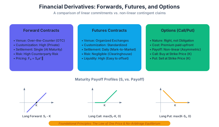
The Future of Finance and Society
Key concepts: AI Financial Advisors · Fiduciary Responsibility · Financial Literacy · Healthcare Finance · Global Decarbonization
Exploration of the evolving role of finance in addressing global challenges and the impact of technology.
The Future of Finance and Society
Overview
In the traditional pedagogical framework of Finance Theory I, the discipline is often presented as a set of tools for maximizing shareholder value or optimizing individual portfolios. However, as we move into the mid-21st century, the scope of financial engineering has expanded. Led by the insights of Professor Andrew Lo and the evolution of the Adaptive Markets Hypothesis (AMH), finance is increasingly viewed as a "functional" technology—a mechanism for coordinating human behavior to solve "wicked problems" that are too large for any single government or corporation to tackle alone.
This section explores the frontier where quantitative finance meets societal evolution. We examine the transition from human-centric fiduciary models to AI-driven financial advisory, the elevation of financial literacy to a fundamental human right, and the application of structured finance to existential challenges like oncology R&D and global decarbonization.
AI_SVGI_SVGThe Infographic depicts the "Financial Engineering Pipeline for Social Impact," showing the flow from individual financial literacy to AI-mediated capital allocation, leading to large-scale funding for healthcare (Megafunds) and climate (Green Bonds).*
AI Financial Advisors and the Evolution of Fiduciary Responsibility
The democratization of finance has historically been limited by the "advice gap"—the high cost of human financial advisors makes professional wealth management inaccessible to the bottom 90% of the wealth distribution. Artificial Intelligence (AI) promises to close this gap, but it introduces a profound legal and ethical challenge: Fiduciary Responsibility.
What it is
A Fiduciary Duty is a legal obligation of one party (the fiduciary) to act in the best interest of another (the principal). In finance, this traditionally involves the Prudent Person Rule, requiring advisors to manage assets with the care, skill, and diligence that a "prudent person" would exercise.
The Mechanics of AI Fiduciary
An AI financial advisor is not merely a chatbot; it is a multi-agent system that integrates a client's Utility Function $U(W)$ with real-time market data. The challenge lies in translating "best interest" into a mathematical constraint within an optimization algorithm.
Definition: The Algorithmic Fiduciary Constraint An AI agent $A$ satisfies the fiduciary constraint if, for every action $a \in \mathcal{A}$, the expected utility $E[U(W) | a]$ is maximized subject to the client's risk tolerance $\sigma_p \leq \sigma_{max}$ and specific ethical constraints (e.g., ESG preferences), without regard to the agent's own fee structure.
Comparison of Advisory Models
| Feature | Traditional Human Advisor | Robo-Advisor (Static) | AI Financial Advisor (Generative/Adaptive) |
|---|---|---|---|
| Scalability | Low (1:100 clients) | High (1:Millions) | High (1:Millions) |
| Personalization | High (Qualitative) | Low (Standardized Portfolios) | Hyper-High (Behavioral Integration) |
| Fiduciary Basis | Legal/Ethical Code | Programmatic Rules | Dynamic Optimization + Explainability |
| Cost | 1.00% - 1.50% AUM | 0.25% - 0.50% AUM | < 0.10% AUM |
| Bias | Cognitive/Emotional | Selection Bias in Data | Algorithmic/Black-box Risk |
Common Pitfalls: The "Black Box" Problem
The primary risk in AI-driven finance is the lack of interpretability. If a Deep Learning model shifts a client's entire portfolio into 10-year Treasuries, the fiduciary must be able to explain why. Without "Explainable AI" (XAI), the model fails the legal test of transparency required in probate and civil courts.
Financial Literacy as a Universal Language
Professor Andrew Lo often describes finance as a "universal language" for navigating life's trade-offs. In this view, financial literacy is not just about balancing a checkbook; it is about understanding the Time Value of Money (TVM) and Risk-Adjusted Returns in every life decision.
The NPV of Life Decisions
Most major life milestones—choosing a college major, buying a home, or selecting a healthcare plan—are essentially Capital Budgeting problems.
Worked Example: The NPV of a Graduate Degree Consider a professional deciding whether to pursue an MBA.
- Cost ($C_0$): $150,000 (Tuition + Opportunity Cost of lost salary).
- Incremental Salary ($CF$): $40,000 per year for 30 years.
- Discount Rate ($r$): 6% (reflecting the risk of the career path).
$$NPV = -150,000 + \sum_{t=1}^{30} \frac{40,000}{(1.06)^t}$$
Using the annuity formula: $$NPV = -150,000 + 40,000 \left[ \frac{1 - (1.06)^{-30}}{0.06} \right]$$ $$NPV = -150,000 + 40,000(13.76) = -150,000 + 550,400 = $400,400$$
A positive NPV suggests the investment is financially sound. However, financial literacy requires adjusting for idiosyncratic risk (e.g., the probability of not completing the degree).
Financial Literacy Framework
| Concept | Societal Application | Individual Misconception |
|---|---|---|
| Compounding | Retirement Security | Underestimating the "cost of waiting" |
| Diversification | Labor Market Resilience | "Putting all eggs" in a single company stock |
| Inflation | Purchasing Power Protection | Confusing nominal gains with real gains |
| Leverage | Home Ownership/Education | Viewing debt only as a burden, not a tool |
Healthcare Finance: The "Megafund" Revolution
One of the most significant applications of Finance Theory I is in the realm of biomedical R&D. The current "Valley of Death" in drug development occurs because individual biotech projects have a high probability of failure, making them unappealing to traditional equity investors.
The Problem: Binary Risk
A single oncology drug trial has a success probability ($p$) of roughly 5-10%. For a venture capitalist, this is a "binary bet" with extreme volatility.
The Solution: Portfolio Theory and Securitization
By applying Portfolio Theory, we can aggregate 100 independent drug trials into a single Megafund. While any single trial is likely to fail, the portfolio as a whole has a highly predictable success rate due to the Law of Large Numbers.
Mathematical Derivation: Probability of Success in a Megafund If $n$ is the number of independent trials and $p$ is the probability of success for each, the probability of at least $k$ successes follows a Binomial Distribution. The probability of zero successes is $(1-p)^n$. Therefore, the probability of at least one success is $1 - (1-p)^n$.
For $n=100$ and $p=0.05$: $$P(\text{at least 1 success}) = 1 - (0.95)^{100} \approx 1 - 0.0059 = 99.41%$$
By pooling these risks, the Megafund can issue Research Backed Obligations (RBOs)—debt instruments that appeal to pension funds and insurance companies looking for steady, uncorrelated returns.
Implementation: A Python Simulation of Megafund Diversification
The following code demonstrates how increasing the number of independent biomedical projects reduces the variance of the outcome, making the "Megafund" investable for debt markets.
import numpy as np
import matplotlib.pyplot as plt

def simulate_megafund(n_projects, p_success, payout_per_success, cost_per_project):
    # Simulate binary outcomes for n projects
    outcomes = np.random.binomial(1, p_success, n_projects)
    total_revenue = np.sum(outcomes) * payout_per_success
    total_cost = n_projects * cost_per_project
    return total_revenue - total_cost

# Parameters
p = 0.05  # 5% success rate
cost = 100  # $100M per drug
payout = 2000 # $2B per successful drug

# Compare a small fund (5 projects) vs a Megafund (100 projects)
small_fund = [simulate_megafund(5, p, payout, cost) for _ in range(10000)]
mega_fund = [simulate_megafund(100, p, payout, cost) for _ in range(10000)]

print(f"Small Fund - Mean: {np.mean(small_fund):.2f}, StdDev: {np.std(small_fund):.2f}")
print(f"Mega Fund - Mean: {np.mean(mega_fund):.2f}, StdDev: {np.std(mega_fund):.2f}")
AI_DEMOI_DEMOThe interactive simulation allows users to adjust the probability of drug success ($p$) and the number of projects ($n$) to see how the "Efficient Frontier" of a healthcare portfolio shifts, demonstrating the point at which the portfolio becomes "investment grade."*
Global Decarbonization and the Cost of Capital
The transition to a net-zero economy is fundamentally a reallocation of capital. The "Green Premium"—the additional cost of choosing a clean technology over a fossil-fuel-based one—is often driven by the higher Cost of Capital for unproven green technologies.
Hurdle Rates and the Energy Transition
In Capital Budgeting, a project is only undertaken if its IRR exceeds the Hurdle Rate (the minimum acceptable return). Green projects (like offshore wind or green hydrogen) often have high upfront CAPEX and low OPEX, making them extremely sensitive to interest rates.
Financial Engineering Tools for Climate
To accelerate decarbonization, financial engineers use several "de-risking" mechanisms:
- Green Bonds: Fixed-income securities where the proceeds are earmarked for environmental projects. They often trade at a "Greenium" (a lower yield than equivalent brown bonds), lowering the issuer's cost of debt.
- Blended Finance: Using public or philanthropic capital to take the "first loss" position in a capital stack, thereby making the remaining tranches safe enough for institutional investors.
- Carbon Credits and Derivatives: Creating a liquid market for carbon allows firms to hedge their transition risk.
Comparison of Climate Finance Instruments
| Instrument | Primary Mechanism | Target Investor | Risk Profile |
|---|---|---|---|
| Green Bonds | Lowering $r$ via "Greenium" | Institutional (Pension/ESG) | Low (Investment Grade) |
| Venture Climate Tech | Equity funding for R&D | VC / Family Offices | High (Binary Risk) |
| Carbon Offsets | Internalizing Externalities | Corporations (Net-Zero goals) | Variable (Regulatory Risk) |
| Catastrophe Bonds | Hedging physical climate risk | Hedge Funds / Reinsurers | High (Event-driven) |
The Adaptive Markets Perspective
The common thread across these topics is the Adaptive Markets Hypothesis (AMH). Unlike the Efficient Markets Hypothesis (EMH), which assumes markets are always rational and efficient, AMH suggests that markets evolve.
- Competition and Mutation: Financial products (like the Megafund) are "mutations" that survive if they provide a better fit for the current environment (e.g., a world with high cancer rates but low interest rates).
- Ecology of Finance: The "Future of Finance" is an ecosystem where AI, regulators, and individual investors interact. When the environment changes (e.g., a global pandemic or climate shift), the financial system must adapt its valuation models.
Key Insight: The Financial Engineer as a Social Architect In the AMH framework, the financial engineer's role is not just to find alpha, but to design the "evolutionary environment" (market structures and incentives) that directs capital toward human flourishing.
AI_FLASHCARDSI_FLASHCARDS Fiduciary Duty: The legal obligation to act in the principal's best interest.
- Megafund: A large-scale investment vehicle that pools high-risk, high-reward projects (like drug trials) to achieve a predictable return through diversification.
- Greenium: The yield spread between a green bond and a conventional bond; the "discount" an issuer receives for being environmentally friendly.
- Blended Finance: The strategic use of development finance and philanthropic funds to mobilize private capital flows to emerging markets.
- Adaptive Markets Hypothesis (AMH): A theory that combines principles of evolution with financial economics to explain market behavior.
- Time Value of Money (TVM): The concept that money available at the present time is worth more than the identical sum in the future due to its potential earning capacity.
AI_QUIZI_QUIZ. True/False: A Megafund reduces the probability of a single drug trial failing. Answer: False. It reduces the impact of a single failure on the overall portfolio return, but the idiosyncratic risk of the trial remains the same. 2. Calculation: If a Green Bond has a yield of 3.8% and an identical "Brown Bond" has a yield of 4.1%, what is the "Greenium"? Answer: 30 basis points (0.30%). 3. Conceptual: Why is AI uniquely suited to solve the "advice gap" in financial literacy? Answer: Because it scales the marginal cost of personalized fiduciary advice to near zero, allowing low-net-worth individuals to access sophisticated optimization. 4. Application: In the context of the NPV of a degree, how does an increase in the discount rate ($r$) affect the decision to attend? Answer: It decreases the NPV, making the investment less attractive, as future incremental earnings are worth less in today's terms.
AI_STUDY_GUIDEI_STUDY_GUIDE*Core Learning Objectives:**
- Contrast the traditional fiduciary model with the emerging requirements for Algorithmic Fiduciary Responsibility.
- Apply the principles of Portfolio Theory (diversification, Law of Large Numbers) to non-traditional assets like biomedical R&D.
- Analyze how the cost of capital ($r$) acts as a primary lever in the global transition to sustainable energy.
- Understand the role of financial literacy as a tool for personal and societal risk management.
Key Equations to Master:
- NPV of a Life Decision: $NPV = \sum \frac{CF_t}{(1+r)^t} - Initial Investment$
- Megafund Success Probability: $P(k \geq 1) = 1 - (1-p)^n$
- Risk-Adjusted Return (Sharpe Ratio): $S = \frac{R_p - R_f}{\sigma_p}$ (Essential for comparing AI-managed portfolios).
Further Reading:
- Adaptive Markets by Andrew Lo (2017).
- "Buying Cures vs. Renting Health" - Research on the securitization of gene therapies.
- The Stern Review on the Economics of Climate Change (focus on discount rate selection).
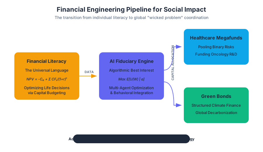
Course Synthesis and Assessment
Key concepts: Midterm Review · Final Exam Preparation · Problem Set Solutions · Case Studies
Comprehensive review materials and assessments to master the course content.
Course Synthesis and Assessment
The culmination of Finance Theory I represents a transition from understanding isolated financial instruments to mastering a unified framework of valuation, risk management, and capital allocation. Assessment in this course—specifically through the Midterm and Final Examinations—is designed not merely to test rote memorization of formulas, but to evaluate a student's ability to apply the Law of One Price across diverse market conditions.
This section synthesizes the core pillars of the curriculum: the Time Value of Money (TVM), Fixed-Income Analysis, Equity Valuation, Portfolio Theory, the Capital Asset Pricing Model (CAPM), and Derivative Pricing. By examining the patterns found in problem sets and past exams, students can develop a heuristic for solving complex financial puzzles under time constraints.
AI_SVGI_SVG## The Midterm Pillar: Foundations and Fixed Income
The midterm assessment focuses on the "physics" of finance: the deterministic mechanics of cash flow timing and the valuation of contractually obligated payments (bonds).
Time Value of Money (TVM) and Arbitrage
At the heart of the midterm is the Net Present Value (NPV) rule. The assessment tests the ability to collapse disparate cash flows into a single point in time using appropriate discount rates. A recurring theme is the distinction between the Annual Percentage Rate (APR) and the Effective Annual Rate (EAR).
The No-Arbitrage Principle: In a well-functioning market, two investments that offer the same certain cash flows must have the same price. If they do not, an arbitrage opportunity exists, which market participants will quickly exploit until prices align.
Common Exam Pattern: Converting non-annual compounding periods into EAR to compare investment vehicles.
- Formula: $EAR = (1 + \frac{APR}{m})^m - 1$, where $m$ is the number of compounding periods per year.
Fixed-Income Securities and the Term Structure
Assessment of fixed income requires navigating the relationship between bond prices, yields, and interest rate sensitivity. Students are expected to derive the Spot Rate Curve from a series of coupon-bearing bonds using "bootstrapping" and to calculate Macaulay and Modified Duration.
| Concept | Definition | Exam Application |
|---|---|---|
| Yield to Maturity (YTM) | The internal rate of return (IRR) of a bond if held to maturity. | Used as a single "average" discount rate for all cash flows. |
| Spot Rate ($r_t$) | The yield on a zero-coupon bond maturing at time $t$. | Used for precise valuation of individual cash flows. |
| Forward Rate ($f_{t,t+1}$) | The interest rate for a period starting in the future, agreed upon today. | Used to test the Expectations Hypothesis vs. Liquidity Preference. |
| Modified Duration ($D^*$) | The percentage change in price for a 100 basis point change in yield. | Measuring interest rate risk; $ \Delta P/P \approx -D^* \times \Delta y $. |
Example Problem: Bond Arbitrage
Problem: A 2-year zero-coupon bond with a face value of $1,000 is trading at $920. A 1-year zero-coupon bond is trading at $960. A 2-year 10% annual coupon bond is trading at $1,050. Is there an arbitrage opportunity?
Solution:
- Calculate the 1-year spot rate ($r_1$): $960 = 1000 / (1+r_1) \Rightarrow r_1 = 4.17%$.
- Calculate the 2-year spot rate ($r_2$): $920 = 1000 / (1+r_2)^2 \Rightarrow r_2 = 4.26%$.
- Calculate the "fair" price of the 2-year coupon bond using spot rates: $P = \frac{100}{(1.0417)^1} + \frac{1100}{(1.0426)^2} = 96.00 + 1012.00 = 1108.00$.
- Conclusion: The market price ($1,050) is lower than the theoretical price ($1,108). You should buy the coupon bond and "strip" it or short the equivalent zeros.
The Final Pillar: Risk, Portfolios, and Derivatives
The final exam shifts the focus from certainty to uncertainty. It introduces the Mean-Variance Framework and the pricing of contingent claims (options).
Portfolio Theory and CAPM
The assessment evaluates the transition from individual asset risk (Standard Deviation) to systematic risk (Beta). Students must demonstrate mastery of the Efficient Frontier and the Capital Market Line (CML).
- Idiosyncratic Risk: Risk that can be diversified away.
- Systematic Risk: Market-wide risk that cannot be diversified; the only risk compensated by higher expected returns in CAPM.
The Separation Theorem: Investors will all hold the same portfolio of risky assets (the Market Portfolio) regardless of their risk aversion, adjusting their total risk only by changing the proportion of their wealth held in the risk-free asset.
| Metric | Formula | Significance |
|---|---|---|
| Portfolio Variance | $\sigma_p^2 = w_A^2\sigma_A^2 + w_B^2\sigma_B^2 + 2w_Aw_B\sigma_A\sigma_B\rho_{AB}$ | Shows how correlation ($\rho$) drives diversification. |
| Beta ($\beta$) | $\beta_i = \frac{Cov(r_i, r_m)}{\sigma_m^2}$ | Measures sensitivity to market movements. |
| CAPM (SML) | $E[r_i] = r_f + \beta_i(E[r_m] - r_f)$ | Defines the "required" return for a given level of risk. |
Derivatives: Forwards, Futures, and Options
Assessment in derivatives centers on the Binomial Option Pricing Model and Put-Call Parity. The key insight tested is "Risk-Neutral Valuation"—the idea that we can price derivatives by creating a synthetic, risk-free hedge.
Put-Call Parity Formula: $C + \frac{K}{(1+r)^T} = P + S_0$
- $C$: Call Price
- $P$: Put Price
- $K$: Strike Price
- $S_0$: Current Stock Price
Common Pitfall: Forgetting to discount the strike price ($K$) in the Put-Call Parity equation.
Capital Budgeting: The Synthesis of Theory and Practice
Capital budgeting is often the bridge between the midterm and final concepts. It requires calculating project cash flows (Midterm) and determining the appropriate discount rate via CAPM (Final).
Incremental Cash Flow Analysis
Exams frequently include "distractor" information. Students must distinguish between relevant and irrelevant costs:
- Sunk Costs: (e.g., past R&D) — Ignore.
- Opportunity Costs: (e.g., using land the firm already owns) — Include.
- Side Effects: (e.g., cannibalization of existing product sales) — Include.
- Depreciation Tax Shield: ($Depreciation \times Tax Rate$) — Include (it is a cash inflow).
Project Valuation Code Example
In modern financial analysis, these calculations are often automated to allow for sensitivity analysis (e.g., varying the WACC or growth rates).
import numpy as np

def calculate_project_metrics(investment, cash_flows, tax_rate, depreciation, discount_rate):
    """
    Calculates NPV and IRR for a project including the Depreciation Tax Shield.
    """
    # Adjust cash flows for taxes and add tax shield
    after_tax_cf = [cf * (1 - tax_rate) + (depreciation * tax_rate) for cf in cash_flows]

    # Prepend the initial investment (negative)
    full_cf_stream = [-investment] + after_tax_cf

    # Calculate NPV
    npv = np.npv(discount_rate, full_cf_stream)

    # Calculate IRR
    irr = np.irr(full_cf_stream)

    return {"NPV": npv, "IRR": irr}

# Example Usage:
# $1M investment, $300k annual cash flow for 5 years, 30% tax, $200k annual depreciation, 10% WACC
metrics = calculate_project_metrics(1000000, [300000]*5, 0.30, 200000, 0.10)
print(f"Project NPV: ${metrics['NPV']:,.2f}")
print(f"Project IRR: {metrics['IRR']:.2%}")
Exam Strategy and Problem-Solving Heuristics
Professor Andrew Lo’s exams are known for requiring "Financial Intuition" alongside mathematical precision. Success requires a specific tactical approach.
1. The "True/False with Justification" Pattern
Many exam sections present a statement and ask if it is True, False, or Uncertain.
- Strategy: If the statement is False, provide a counter-example. If it is True, cite a specific theorem (e.g., "By the Modigliani-Miller Theorem...").
- Example: "A stock with a negative Beta must have a negative expected return."
- Answer: False. According to CAPM, $E[r] = r_f + \beta(E[r_m] - r_f)$. If $\beta$ is negative, the expected return is less than the risk-free rate, but it can still be positive if $r_f$ is sufficiently high.
2. Multi-Stage Growth Models
When valuing equities, exams often move beyond the Gordon Growth Model ($P = \frac{D_1}{r-g}$) to multi-stage models where growth is high for $n$ years and then stabilizes.
- Heuristic: Calculate the individual PV of dividends during the high-growth phase, then calculate the "Terminal Value" at the start of the stable phase and discount it back to the present.
3. Sensitivity to Assumptions
In case studies, the "correct" answer often depends on the assumptions made about market efficiency.
- EMH (Efficient Market Hypothesis): Prices reflect all available information. NPV of any trade is zero.
- Adaptive Markets Hypothesis: Market efficiency is not a binary state but an evolutionary process. Prices can diverge from fundamentals due to behavioral biases.
| Valuation Method | Best Used For... | Key Weakness |
|---|---|---|
| Dividend Discount Model (DDM) | Stable, dividend-paying firms. | Useless for high-growth tech firms with no dividends. |
| Free Cash Flow (FCF) | Firms with irregular dividends or high reinvestment. | Highly sensitive to Terminal Value assumptions. |
| Comparables (Multiples) | Quick "sanity checks" against peers. | Ignores firm-specific risk and growth nuances. |
Case Study Synthesis: Drug Development Finance
A unique aspect of the MIT 15.401 curriculum is the application of finance to "non-financial" sectors like biotech.
The Problem: High failure rates in drug trials make individual projects "un-investable" for traditional equity. The Synthesis: By applying Portfolio Theory, we can bundle 100 independent drug trials into a single "Mega-Fund."
- While each trial has a 95% failure rate, the probability of at least one success in a bundle of 100 is $1 - (0.95)^{100} \approx 99.4%$.
- This transforms high-risk idiosyncratic bets into a statistically predictable investment, allowing for the use of Securitization (debt financing) to fund medical breakthroughs.
Common Pitfalls in Assessment
- Mixing Real and Nominal Rates: Always ensure that if cash flows are nominal (include inflation), the discount rate is also nominal. $1 + r_{nominal} = (1 + r_{real})(1 + i)$.
- Confusing the CML and SML:
- The Capital Market Line (CML) plots expected return against total risk ($\sigma$) for efficient portfolios.
- The Security Market Line (SML) plots expected return against systematic risk ($\beta$) for any asset or portfolio.
- Incorrect Timing of Cash Flows: In annuity formulas, the first payment is assumed to happen at $t=1$. If a payment happens at $t=0$ (Annuity Due), you must multiply the result by $(1+r)$.
- Ignoring the "Margin of Safety" in Options: When using the Binomial Model, ensure the "No-Arbitrage" condition $d < (1+r) < u$ is met; otherwise, the risk-neutral probabilities will be invalid.
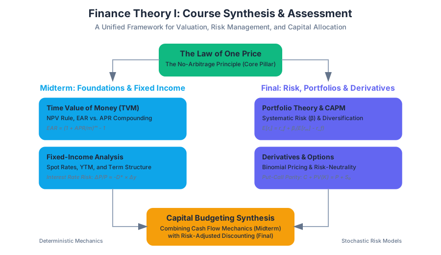
Source Materials
Study Finance Theory I with AI — Free on Lykke
Sign up for free to generate personalized flashcards, quizzes, and study guides from this course. Chat with an AI tutor that knows the material.
Get Started FreeView this course wiki on Lykke · Browse all public course wikis