Econometric Theory and Empirical Analysis with Stata
Institution: MIT
47 study materials · 7 sections
This course provides a comprehensive introduction to econometrics, focusing on the application of statistical methods to economic data to estimate causal relationships and test theories. Students learn the theoretical foundations of Ordinary Least Squares (OLS), the Gauss-Markov assumptions, and statistical inference within both simple and multiple regression frameworks. The curriculum also covers advanced topics such as instrumental variables, difference-in-differences, and heteroskedasticity, all integrated with practical data analysis using Stata software.
Course Sections
Introduction and Statistical Foundations
Key concepts: Ceteris Paribus · Causality vs. Correlation · Empirical Analysis Steps · Counterfactuals
Establishes the definition of econometrics and the fundamental distinction between causality and correlation, alongside a review of essential statistical concepts.
Introduction and Statistical Foundations
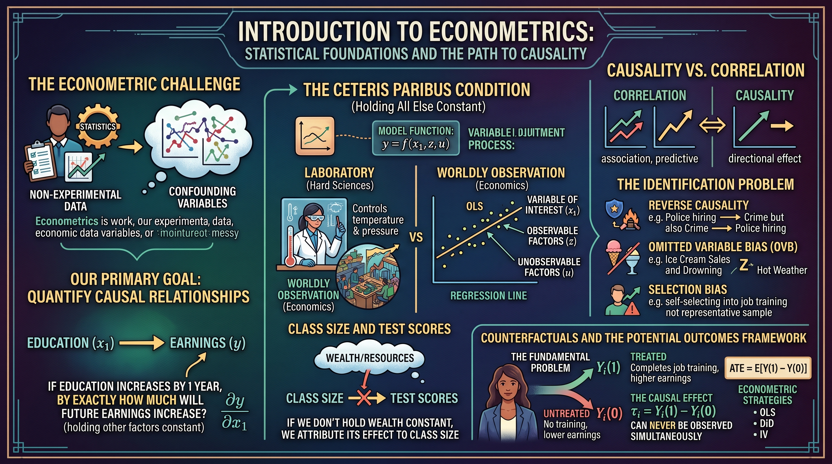
Econometrics is the rigorous application of mathematical and statistical methods to the analysis of economic data. While it shares a lineage with mathematical statistics, econometrics is a distinct discipline because it focuses on the unique challenges of non-experimental data. In the hard sciences, researchers can often control the environment; in economics, we observe the world as it is, fraught with confounding variables and complex interdependencies.
The primary goal of econometrics is not merely to find patterns, but to quantify causal relationships. We do not just ask if education and earnings move together; we ask: "If we increase a person's education by one year, by exactly how much will their future earnings increase, holding all other factors constant?"
The Ceteris Paribus Condition
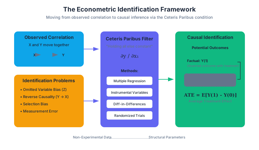
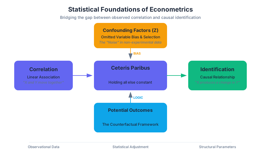
The cornerstone of economic theory and econometric estimation is the Ceteris Paribus condition—a Latin phrase meaning "holding all else constant." In a laboratory, a chemist can hold temperature and pressure constant while varying a catalyst. In economics, we must use statistical techniques to mimic this control.
The Mathematical Representation
In a functional relationship $y = f(x_1, x_2, ..., x_n)$, the effect of $x_1$ on $y$ is defined by the partial derivative: $$\frac{\partial y}{\partial x_1}$$ This derivative represents the change in $y$ for a marginal change in $x_1$, assuming $x_2$ through $x_n$ remain unchanged. In econometrics, our models explicitly partition the world into the variable of interest ($x$), other observable factors ($z$), and unobservable factors ($u$).
Why Ceteris Paribus is Difficult
In observational data, variables are rarely independent. If we want to measure the effect of "Class Size" on "Student Test Scores," we face the problem that wealthier school districts often have both smaller classes and more resources at home. If we simply compare small classes to large classes without "holding constant" family income, we attribute the effect of wealth to class size.
| Data Type | Control Mechanism | Primary Challenge |
|---|---|---|
| Experimental | Random Assignment | Cost, Ethics, External Validity |
| Observational | Statistical Adjustment (Regression) | Omitted Variable Bias, Endogeneity |
| Quasi-Experimental | Natural Shocks (DiD, IV) | Finding a "clean" natural experiment |
Causality vs. Correlation
A common mantra in statistics is that "correlation does not imply causation." Econometrics takes this a step further by defining exactly why they differ and how to close the gap.
- Correlation: A measure of the linear association between two variables. If $X$ and $Y$ are correlated, knowing $X$ helps us predict $Y$.
- Causality: A directional relationship where a change in $X$ produces a change in $Y$.
The Identification Problem
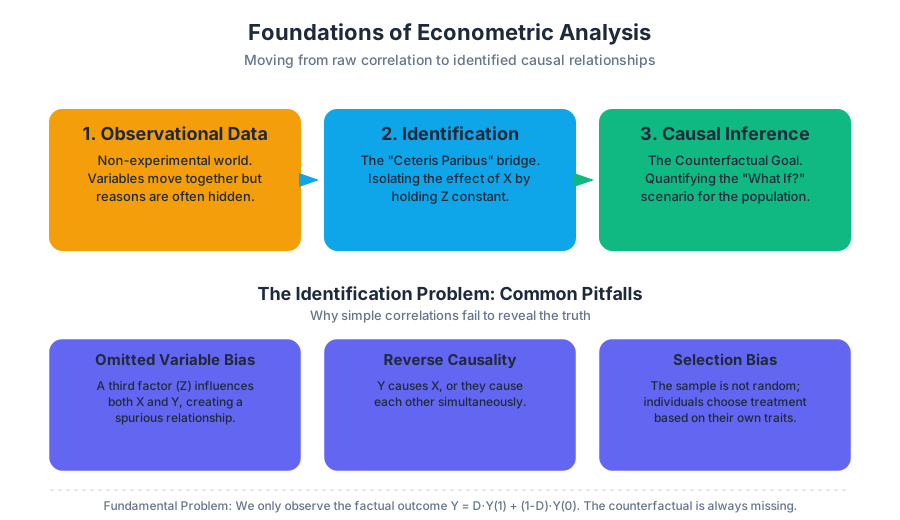
The central struggle in econometrics is Identification. We say a causal effect is "identified" if we can isolate it from the noise of other correlations. Consider the relationship between police presence and crime rates. A simple correlation might show that cities with more police have higher crime. A naive observer might conclude police cause crime. In reality, the causality is reversed: high-crime cities hire more police. This is known as Simultaneous Equation Bias.
Common Pitfalls in Causal Logic
- Reverse Causality: $Y$ causes $X$ instead of $X$ causing $Y$.
- Omitted Variable Bias (OVB): A third variable $Z$ causes both $X$ and $Y$, creating a "spurious" correlation.
- Selection Bias: The sample is not representative, or individuals "self-select" into the treatment group based on characteristics that also affect the outcome.
Counterfactuals and the Potential Outcomes Framework
To understand causality, we must think in terms of Counterfactuals. A counterfactual asks: "What would have happened to this specific individual if they had received a different treatment?"
The Potential Outcomes Notation
Let $Y_i(1)$ be the outcome for individual $i$ if they receive the treatment (e.g., a job training program), and $Y_i(0)$ be the outcome if they do not. The Causal Effect for individual $i$ is: $$\tau_i = Y_i(1) - Y_i(0)$$
The Fundamental Problem of Causal Inference is that we can never observe both $Y_i(1)$ and $Y_i(0)$ for the same person at the same time. We only observe the "factual" outcome: $$Y_i = D_i Y_i(1) + (1 - D_i) Y_i(0)$$ where $D_i$ is a binary indicator (1 if treated, 0 if not).
Average Treatment Effect (ATE)
Since we cannot calculate $\tau_i$ for individuals, we aim for the population average: $$ATE = E[Y(1) - Y(0)]$$ Econometric methods like OLS, Difference-in-Differences, and Instrumental Variables are all different strategies to estimate this ATE by constructing a valid proxy for the missing counterfactual.
import numpy as np
import pandas as pd

# Low-level implementation: Simulating Potential Outcomes and Selection Bias
def simulate_causal_data(n=1000):
    # 1. Generate unobserved ability (the 'u' in our model)
    ability = np.random.normal(10, 2, n)

    # 2. Treatment assignment (Education) is NOT random
    # People with higher ability are more likely to get more education
    education = 0.5 * ability + np.random.normal(8, 1, n)

    # 3. Define Potential Outcomes
    # Wage if Education = x: Wage = 5 + 2*Education + 1*Ability + noise
    # Note: Ability affects both Education and Wage (Omitted Variable Bias)
    noise = np.random.normal(0, 1, n)
    wage = 5 + 2 * education + 1 * ability + noise

    df = pd.DataFrame({
        'wage': wage,
        'education': education,
        'ability': ability # In the real world, we wouldn't see this!
    })

    # Simple Correlation (Biased)
    naive_beta = df['wage'].cov(df['education']) / df['education'].var()

    # True Causal Effect (from our formula above) is 2.0
    print(f"Naive OLS Estimate: {naive_beta:.4f}")
    print(f"True Causal Effect: 2.0000")

    return df

simulate_causal_data()
The Empirical Analysis Process
A structured econometric study follows a specific pipeline. It is not enough to simply "run a regression"; one must ground the analysis in theory and data integrity.
Steps in Empirical Analysis
- Question Formulation: Define a narrow, testable hypothesis (e.g., "Does reducing class size by 10% increase test scores?").
- Economic Model: Write down a theoretical framework. This might be a utility maximization problem or a simple behavioral assumption.
- Econometric Model: Convert the economic model into a functional form that can be estimated.
- Example: $Score = \beta_0 + \beta_1 ClassSize + \beta_2 Income + u$
- Data Collection: Identify the population, sampling scheme, and unit of observation.
- Estimation: Use software (like Stata or R) to calculate the parameters ($\hat{\beta}$).
- Hypothesis Testing: Determine if the results are statistically significant or likely due to chance.
| Step | Goal | Common Tool |
|---|---|---|
| Specification | Define the relationship | Linear Regression Equation |
| Identification | Ensure $\beta$ is causal | Instrumental Variables, Fixed Effects |
| Inference | Test significance | t-stats, p-values, F-tests |
| Diagnostics | Check assumptions | Residual plots, Breusch-Pagan test |
Simple Linear Regression (SLR) Foundations
The Simple Linear Regression model is the workhorse of econometrics. It relates a dependent variable $y$ to a single independent variable $x$ via the equation: $$y = \beta_0 + \beta_1 x + u$$
The Gauss-Markov Assumptions (SLR.1 - SLR.4)
To ensure that our OLS estimators ($\hat{\beta}_0, \hat{\beta}_1$) are unbiased (meaning that on average, they hit the true population parameter), four assumptions must hold:
- SLR.1: Linear in Parameters: The population model must be linear in $\beta_0$ and $\beta_1$. (Note: $x$ can be non-linear, like $x^2$).
- SLR.2: Random Sampling: The data represents a random draw from the population.
- SLR.3: Sample Variation in X: The values of $x$ in our sample cannot all be the same. We need variation to see how $y$ changes.
- SLR.4: Zero Conditional Mean: This is the "Golden Rule." It states that the error term $u$ has an expected value of zero regardless of the value of $x$: $$E[u|x] = 0$$
The Zero Conditional Mean Assumption is the mathematical embodiment of ceteris paribus. If $E[u|x] \neq 0$, it means that some factors hidden in $u$ are correlated with $x$. This violates the "holding all else constant" requirement, leading to biased estimates.
Deriving the OLS Estimator
The goal of Ordinary Least Squares (OLS) is to minimize the Sum of Squared Residuals (SSR).
% Mathematical Derivation of Beta_1
To minimize SSR = \sum (y_i - \hat{\beta}_0 - \hat{\beta}_1 x_i)^2:

1. Take the partial derivative with respect to \hat{\beta}_1:
   \frac{\partial SSR}{\partial \hat{\beta}_1} = -2 \sum x_i (y_i - \hat{\beta}_0 - \hat{\beta}_1 x_i) = 0

2. Solving the system of first-order conditions yields:
   \hat{\beta}_1 = \frac{\sum (x_i - \bar{x})(y_i - \bar{y})}{\sum (x_i - \bar{x})^2}

3. Which is equivalent to:
   \hat{\beta}_1 = \frac{Cov(x, y)}{Var(x)}
Advanced Topic: Multiple Regression and Partialling Out
In the real world, SLR is rarely sufficient because of Omitted Variable Bias. Multiple Linear Regression (MLR) allows us to include multiple control variables: $$y = \beta_0 + \beta_1 x_1 + \beta_2 x_2 + ... + \beta_k x_k + u$$
The "Partialling Out" Interpretation
In a multiple regression, $\beta_1$ has a very specific meaning. It is the effect of $x_1$ on $y$ after the effects of $x_2, ..., x_k$ have been "partialled out" or removed from both $x_1$ and $y$. This is the statistical realization of the ceteris paribus thought experiment.
| Concept | SLR | MLR |
|---|---|---|
| Model | $y = \beta_0 + \beta_1 x + u$ | $y = \beta_0 + \beta_1 x_1 + \beta_2 x_2 + u$ |
| Interpretation | Total association | Partial effect (ceteris paribus) |
| Error Term | Contains all other factors | Contains only factors not in model |
| Bias Risk | High (Omitted variables) | Lower (if controls are good) |
Practical Implementation in Stata
Stata is the industry standard for econometric research due to its robust handling of complex survey data and built-in commands for causal inference.
Standard Workflow
A typical session involves cleaning data, generating new variables (transformations), and running regressions with robust standard errors to account for heteroskedasticity.
// 1. Setup environment
clear all
set more off
capture log close

// 2. Load dataset (Example: Wage and Education)
use "http://www.stata-press.com/data/r15/wage2.dta", clear

// 3. Descriptive Statistics
summarize wage educ exper tenure

// 4. Visualizing the relationship
twoway (scatter wage educ) (lfit wage educ), title("Wage vs Education")

// 5. Simple Linear Regression
regress wage educ

// 6. Multiple Regression with Ceteris Paribus controls
// We add 'exper' (experience) and 'tenure' to hold them constant
regress wage educ exper tenure, robust

// 7. Testing a hypothesis (e.g., does educ coefficient = 100?)
test educ = 100
Common Pitfalls in Empirical Foundations
Even with sophisticated software, researchers often fall into traps that invalidate their causal claims.
1. The Dummy Variable Trap
When using categorical data (e.g., "Gender" or "Region"), one must always omit one category (the "base group"). If you include a dummy for "Male" and a dummy for "Female" along with an intercept, the model will suffer from perfect multicollinearity because $Male + Female = 1$ (the constant).
2. Over-controlling (Bad Controls)
While adding controls is generally good for ceteris paribus, adding "bad controls" can introduce bias. A bad control is a variable that is itself an outcome of the variable of interest. For example, if studying the effect of education on wages, controlling for "Job Title" is problematic because education helps determine your job title.
3. Misinterpreting R-Squared
A high $R^2$ (the fraction of variance explained by the model) does not mean the model is "good" or "causal." In time-series data, two unrelated variables that both trend upward over time will have an $R^2$ near 1.0, despite having zero causal connection. This is known as Spurious Regression.
Summary of Statistical Properties
To wrap up the foundations, we must distinguish between the Estimator (the rule/formula) and the Estimate (the number produced by a specific sample).
- Unbiasedness: $E[\hat{\beta}] = \beta$. On average, the estimator is correct.
- Efficiency: Among all unbiased estimators, the one with the smallest variance is the most efficient.
- Consistency: As the sample size $n$ approaches infinity, the estimate $\hat{\beta}$ collapses to the true population value $\beta$.
The Gauss-Markov Theorem: Under assumptions SLR.1 through SLR.5 (adding Homoskedasticity), the OLS estimator is the BLUE: Best Linear Unbiased Estimator.
Simple Linear Regression Model
Key concepts: OLS Estimators · Zero Conditional Mean · Unbiasedness · SLR.1-SLR.4 · Sampling Distribution
Covers the mechanics of the two-variable regression model, the OLS estimation method, and the assumptions required for unbiasedness.
Simple Linear Regression Model
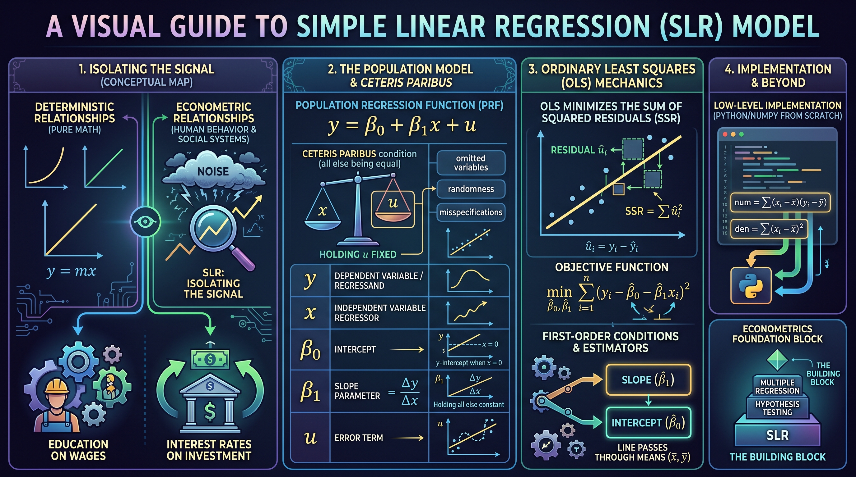
The Simple Linear Regression (SLR) model serves as the foundational building block of econometrics. It provides a formal mathematical framework for estimating the relationship between a dependent variable and a single independent variable. Unlike pure mathematics, where relationships are deterministic, econometrics acknowledges the inherent "noise" in human behavior and social systems. The SLR model attempts to isolate the signal—the systematic relationship between variables—from this noise.
At its core, the SLR model is a tool for empirical analysis, allowing researchers to test economic theories, evaluate policy interventions, and forecast future trends. Whether we are analyzing the impact of education on wages, the effect of interest rates on investment, or the relationship between advertising spend and sales, the SLR model provides the rigorous structure necessary to move from anecdotal observation to statistical inference.
The Population Model and Ceteris Paribus
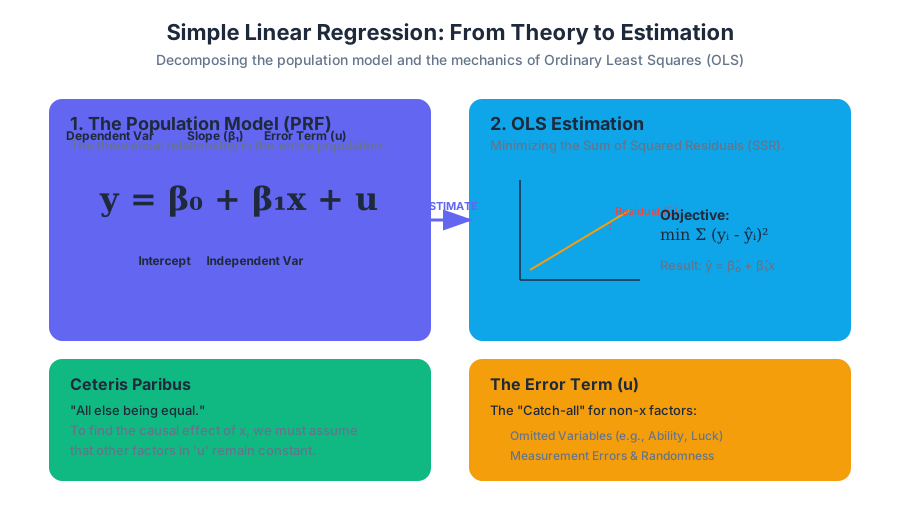
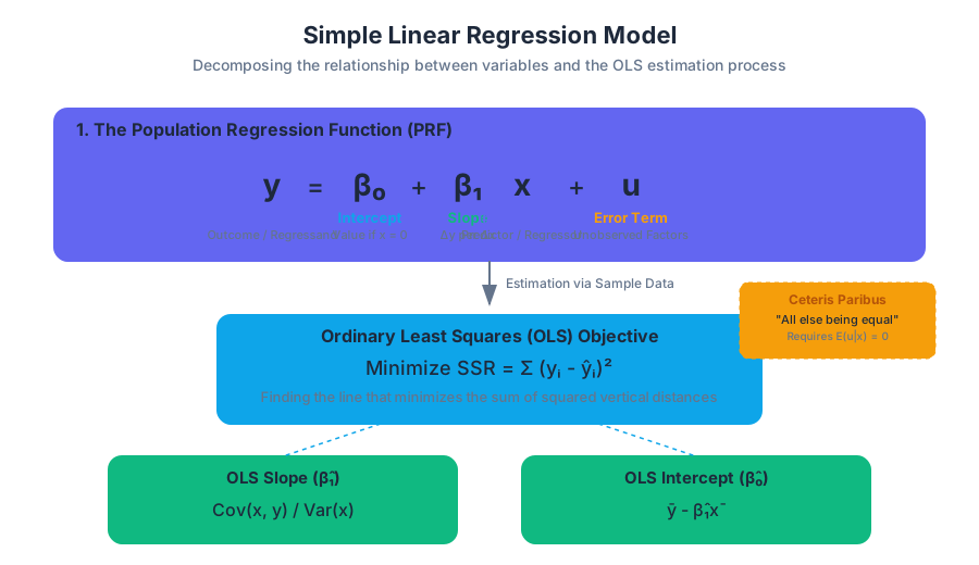
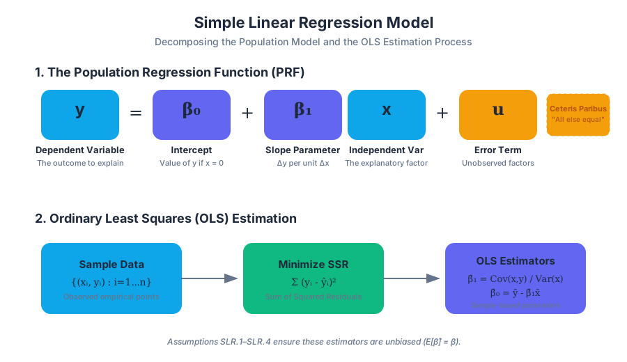
The SLR model describes how a dependent variable $y$ changes as an independent variable $x$ changes in the population. The relationship is expressed by the Population Regression Function (PRF):
$$y = \beta_0 + \beta_1 x + u$$
In this equation, we distinguish between several critical components:
| Component | Term | Definition |
|---|---|---|
| $y$ | Dependent Variable | The variable we are trying to explain (also called the regressand or response variable). |
| $x$ | Independent Variable | The variable used to explain $y$ (also called the regressor, predictor, or explanatory variable). |
| $\beta_0$ | Intercept | The predicted value of $y$ when $x = 0$. |
| $\beta_1$ | Slope Parameter | The change in $y$ for a one-unit change in $x$, holding all other factors constant. |
| $u$ | Error Term | The "disturbance" representing all factors other than $x$ that affect $y$. |
The primary challenge in econometrics is the Ceteris Paribus (all else being equal) condition. Because $u$ contains all other factors affecting $y$, we can only claim that $\beta_1$ represents the causal effect of $x$ on $y$ if we can effectively "hold $u$ fixed." If $x$ is correlated with factors inside $u$, we cannot distinguish the effect of $x$ from the effect of those hidden factors.
Definition: The Error Term ($u$) The error term $u$ is not merely a measurement error. It captures omitted variables, inherent randomness in human behavior, and functional form misspecifications. In a model of
wage = β0 + β1(education) + u, the error term $u$ includes innate ability, work ethic, and family connections.
Ordinary Least Squares (OLS) Mechanics
How do we estimate the unknown parameters $\beta_0$ and $\beta_1$ using a sample of data? The standard method is Ordinary Least Squares (OLS). OLS works by choosing estimates ($\hat{\beta}_0$ and $\hat{\beta}_1$) that minimize the distance between the observed data points and the fitted regression line.
Specifically, OLS minimizes the Sum of Squared Residuals (SSR). For any observation $i$, the residual $\hat{u}_i$ is the difference between the actual value $y_i$ and the predicted value $\hat{y}_i$:
$$\hat{u}_i = y_i - \hat{y}_i = y_i - (\hat{\beta}_0 + \hat{\beta}_1 x_i)$$
The OLS objective function is: $$\min_{\hat{\beta}_0, \hat{\beta}1} \sum{i=1}^{n} (y_i - \hat{\beta}_0 - \hat{\beta}_1 x_i)^2$$
The First-Order Conditions
To find the minimum, we take partial derivatives with respect to $\hat{\beta}_0$ and $\hat{\beta}_1$ and set them to zero. This yields the OLS estimators:
- The Slope ($\hat{\beta}_1$): $\hat{\beta}_1 = \frac{\sum (x_i - \bar{x})(y_i - \bar{y})}{\sum (x_i - \bar{x})^2} = \frac{\text{Cov}(x,y)}{\text{Var}(x)}$
- The Intercept ($\hat{\beta}_0$): $\hat{\beta}_0 = \bar{y} - \hat{\beta}_1 \bar{x}$
These formulas ensure that the regression line passes through the sample means $(\bar{x}, \bar{y})$.
Low-Level Implementation (Python/NumPy)
The following code demonstrates how to implement the OLS closed-form solution from scratch using matrix operations and summation logic.
import numpy as np

def simple_linear_regression(x, y):
    """
    Computes OLS estimators for a simple linear regression.
    Formula: beta_1 = Cov(x,y) / Var(x)
             beta_0 = mean(y) - beta_1 * mean(x)
    """
    n = len(x)
    x_mean = np.mean(x)
    y_mean = np.mean(y)

    # Calculate the numerator (covariance-like) and denominator (variance-like)
    numerator = np.sum((x - x_mean) * (y - y_mean))
    denominator = np.sum((x - x_mean)**2)

    # Slope (beta_1)
    beta_1 = numerator / denominator

    # Intercept (beta_0)
    beta_0 = y_mean - (beta_1 * x_mean)

    # Calculate residuals and R-squared
    y_pred = beta_0 + beta_1 * x
    residuals = y - y_pred
    ssr = np.sum(residuals**2)
    sst = np.sum((y - y_mean)**2)
    r_squared = 1 - (ssr / sst)

    return {
        "intercept": beta_0,
        "slope": beta_1,
        "r_squared": r_squared,
        "residuals": residuals
    }

# Example Usage with synthetic data
x_data = np.array([12, 14, 16, 18, 20]) # Years of Education
y_data = np.array([30, 35, 42, 48, 55]) # Hourly Wage
results = simple_linear_regression(x_data, y_data)

print(f"Model: Wage = {results['intercept']:.2f} + {results['slope']:.2f} * Education")
print(f"R-squared: {results['r_squared']:.4f}")
The Gauss-Markov Assumptions (SLR.1 - SLR.4)
For OLS estimators to be reliable, certain conditions must be met. In the context of "Simple Linear Regression," we focus on the first four Gauss-Markov assumptions, which guarantee that our estimators are unbiased.
SLR.1: Linear in Parameters
The population model must be linear in the parameters $\beta_0$ and $\beta_1$. Note that the variables $x$ and $y$ can be non-linear (e.g., $y = \beta_0 + \beta_1 x^2 + u$), but the coefficients must appear in a linear additive form.
SLR.2: Random Sampling
We have a random sample of $n$ observations ${(x_i, y_i) : i=1, ..., n}$ following the population model. This ensures that the sample is representative of the population we wish to study.
SLR.3: Sample Variation in $x$
The values of $x_i$ in the sample are not all the same. If $x$ is constant, we cannot observe how $y$ changes in response to $x$, and the denominator in the $\hat{\beta}_1$ formula becomes zero, making the estimator undefined.
SLR.4: Zero Conditional Mean
This is the most critical and frequently violated assumption. It states that the error term $u$ has an expected value of zero given any value of $x$: $$E[u|x] = 0$$
If this holds, $x$ is said to be exogenous. If $x$ is correlated with $u$ (i.e., $E[u|x] \neq 0$), then $x$ is endogenous, and the OLS estimator will be biased.
| Assumption | Formal Statement | Violation Consequence | Real-world Example of Violation |
|---|---|---|---|
| SLR.1 | $y = \beta_0 + \beta_1 x + u$ | Model Misspecification | Relationship is exponential, not linear. |
| SLR.2 | ${(x_i, y_i)}$ is IID | Selection Bias | Surveying only wealthy people for a wage study. |
| SLR.3 | $\text{Var}(x) > 0$ | Undefined Estimator | Testing the effect of "Year" using data from only 2023. |
| SLR.4 | $E[u|x] = 0$ | Bias (Inaccuracy) | Omitted variable: "Ability" correlated with "Education". |
Deep Dive: The Zero Conditional Mean Assumption
The assumption $E[u|x] = 0$ implies two things:
- $E[u] = 0$: On average, the factors in the error term cancel out. This is usually trivial because we can always adjust the intercept $\beta_0$ to make this true.
- $\text{Cov}(x, u) = 0$: The unobserved factors are not correlated with the explanatory variable.
Consider the model: $\text{Wage} = \beta_0 + \beta_1 \text{Educ} + u$. If $u$ contains "Ability," and higher-ability individuals tend to get more education, then $\text{Cov}(\text{Educ}, \text{Ability}) > 0$. In this case, OLS will attribute the effect of ability to education, resulting in an "Upward Bias." The estimated $\hat{\beta}_1$ will be larger than the true causal effect $\beta_1$.
Mathematical Derivation of the Slope Estimator
The following block represents the algebraic derivation of the OLS slope estimator, showing how the "Zero Conditional Mean" assumption allows us to identify the population parameter.
1. Start with the definition of covariance:
   Cov(x, y) = Cov(x, beta_0 + beta_1 * x + u)

2. Use covariance properties (linearity):
   Cov(x, y) = Cov(x, beta_0) + Cov(x, beta_1 * x) + Cov(x, u)

3. Simplify:
   - Cov(x, beta_0) = 0 (covariance with a constant is zero)
   - Cov(x, beta_1 * x) = beta_1 * Var(x)
   - Cov(x, u) = 0 (By Assumption SLR.4)

4. Resulting Equation:
   Cov(x, y) = beta_1 * Var(x)

5. Solve for beta_1:
   beta_1 = Cov(x, y) / Var(x)

6. Sample Analog (OLS):
   hat_beta_1 = [Sum(x_i - mean_x)(y_i - mean_y)] / [Sum(x_i - mean_x)^2]
Unbiasedness and the Sampling Distribution
It is vital to distinguish between the Estimator (the rule/formula) and the Estimate (the specific number calculated from a specific sample).
Because the sample is random (SLR.2), $\hat{\beta}_1$ is a random variable. If we took 1,000 different samples from the same population, we would get 1,000 different values for $\hat{\beta}_1$.
Theorem: Unbiasedness of OLS Under assumptions SLR.1 through SLR.4, the OLS estimators are unbiased. That is: $E[\hat{\beta}_0] = \beta_0$ and $E[\hat{\beta}_1] = \beta_1$
Unbiasedness does not mean $\hat{\beta}_1$ will equal $\beta_1$ in any single sample. It means that if we could repeat the sampling process infinitely many times, the average of all those estimates would exactly equal the true population parameter.
Visualizing the Sampling Distribution
The variance of the sampling distribution tells us how "spread out" our estimates are. A smaller variance means our estimator is more precise. The variance of $\hat{\beta}_1$ (under the additional assumption of homoskedasticity) is: $$\text{Var}(\hat{\beta}_1) = \frac{\sigma^2}{\sum (x_i - \bar{x})^2}$$ Where $\sigma^2$ is the variance of the error term $u$.
Goodness of Fit: R-Squared ($R^2$)
Once we have estimated the model, we want to know how well the independent variable $x$ explains the variation in $y$. We decompose the Total Sum of Squares (SST) into two parts:
- SST (Total Sum of Squares): $\sum (y_i - \bar{y})^2$ — Total variation in $y$.
- SSE (Explained Sum of Squares): $\sum (\hat{y}_i - \bar{y})^2$ — Variation explained by the model.
- SSR (Residual Sum of Squares): $\sum \hat{u}_i^2$ — Variation left unexplained.
The relationship is: $SST = SSE + SSR$.
The Coefficient of Determination ($R^2$) is defined as: $$R^2 = \frac{SSE}{SST} = 1 - \frac{SSR}{SST}$$
$R^2$ ranges from 0 to 1. An $R^2$ of 0.30 means that 30% of the variation in $y$ is explained by $x$. In social sciences, $R^2$ is often low (e.g., 0.1 to 0.2) because human behavior is influenced by countless factors outside the model.
| Metric | Formula | Interpretation |
|---|---|---|
| SST | $\sum (y_i - \bar{y})^2$ | The "total uncertainty" in the dependent variable. |
| SSR | $\sum (y_i - \hat{y}_i)^2$ | The "failure" of the model; what we couldn't explain. |
| SSE | $\sum (\hat{y}_i - \bar{y})^2$ | The "success" of the model; the movement in $y$ tracked by $x$. |
| $R^2$ | $SSE / SST$ | Percentage of variance explained (0 to 100%). |
Practical Implementation in Stata
In professional econometrics, software like Stata is the industry standard for performing these calculations. Stata handles the matrix algebra internally and provides robust diagnostic output.
// 1. Load a dataset (e.g., the 'attend' dataset from Wooldridge)
use http://www.stata.com/data/jwooldridge/econtf/attend.dta, clear

// 2. Summarize variables to check SLR.3 (variation in x)
summarize atndrte priGPA

// 3. Visualize the relationship (Scatterplot with regression line)
twoway (scatter atndrte priGPA) (lfit atndrte priGPA)

// 4. Run the Simple Linear Regression
// Syntax: regress [dependent] [independent]
regress atndrte priGPA

/*
Output Interpretation:
- '_cons' is the intercept (beta_0)
- 'priGPA' coefficient is the slope (beta_1)
- 'R-squared' is the goodness of fit
- 'Prob > F' tests if the model is statistically significant
*/

// 5. Predict residuals to check for patterns
predict u_hat, residual
scatter u_hat priGPA, yline(0)
Common Pitfalls and Misconceptions
1. Correlation is Not Causation
Just because $\hat{\beta}_1$ is statistically significant does not mean $x$ causes $y$. If SLR.4 is violated (e.g., omitted variable bias), the coefficient represents both the effect of $x$ and the effect of the correlated unobservables.
2. The "Intercept" Fallacy
Often, the intercept $\beta_0$ has no meaningful economic interpretation. For example, in a regression of weight on height, the intercept represents the weight of a person with zero height. While mathematically necessary to anchor the line, it is often outside the range of observed data.
3. Low $R^2$ Does Not Mean a "Bad" Model
A low $R^2$ is common in cross-sectional data. A researcher might have a very precise and unbiased estimate of a small effect. The goal of econometrics is often to estimate $\beta_1$ accurately, not necessarily to predict $y$ perfectly.
4. Non-Linearity
If the true relationship is a curve (e.g., diminishing marginal returns), a straight line will provide a poor fit and potentially biased estimates of the local effect. This is why visual inspection of data (scatterplots) is a mandatory first step.
Summary of the SLR Workflow
- Specify the Theory: Define $y$ and $x$ and the expected sign of $\beta_1$.
- Collect Data: Ensure the sample is random (SLR.2).
- Inspect Data: Check for variation in $x$ (SLR.3) and potential non-linearity.
- Estimate OLS: Calculate $\hat{\beta}_0$ and $\hat{\beta}_1$.
- Evaluate Assumptions: Critically assess if $E[u|x]=0$ (SLR.4).
- Interpret Results: Use the slope to describe the ceteris paribus effect and $R^2$ to describe the fit.
Multiple Regression: Estimation and Inference
Key concepts: Partial Effects · Omitted Variable Bias · Gauss-Markov Theorem (BLUE) · t-tests · F-tests
Extends the regression framework to multiple independent variables, focusing on partial effects, the Gauss-Markov Theorem, and hypothesis testing.
Multiple Regression: Estimation and Inference
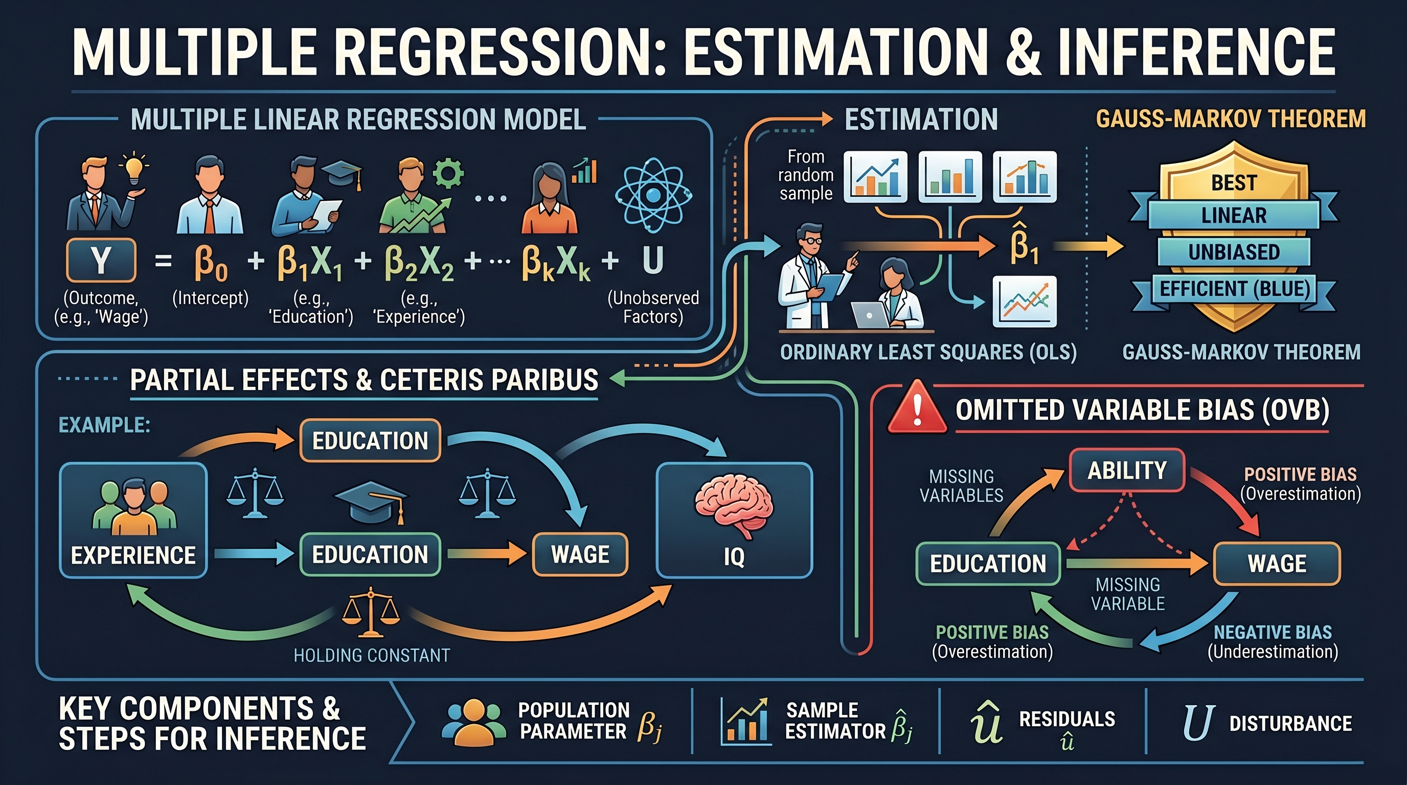
Multiple Linear Regression (MLR) is the cornerstone of empirical economic analysis. While Simple Linear Regression (SLR) provides a foundation, it rarely suffices in the real world where outcomes are driven by a complex web of interrelated factors. The power of MLR lies in its ability to isolate the effect of a single variable while "holding constant" other confounding factors—a concept known as ceteris paribus.
In this deep dive, we move beyond basic correlation to explore how MLR allows for rigorous estimation of partial effects, the dangers of omitting crucial variables, and the statistical framework required to make valid inferences about population parameters.
The Multiple Linear Regression Model
The population model for multiple linear regression with $k$ independent variables is expressed as:
$$y = \beta_0 + \beta_1 x_1 + \beta_2 x_2 + \dots + \beta_k x_k + u$$
Where:
- $y$ is the dependent variable (the outcome we wish to explain).
- $x_1, x_2, \dots, x_k$ are the independent variables (regressors or predictors).
- $\beta_0$ is the intercept (the value of $y$ if all $x$ are zero).
- $\beta_1, \dots, \beta_k$ are the slope parameters (measuring the partial effect of each $x$).
- $u$ is the error term (representing unobserved factors affecting $y$).
| Component | Description | Role in Inference |
|---|---|---|
| $\beta_j$ | Population Parameter | The "true" relationship we seek to estimate. |
| $\hat{\beta}_j$ | OLS Estimator | The sample-based estimate of the population parameter. |
| $u$ | Disturbance/Error | The source of uncertainty; must satisfy Gauss-Markov assumptions. |
| $\hat{u}$ | Residual | The difference between observed $y$ and predicted $\hat{y}$. |
Partial Effects: The "Ceteris Paribus" Interpretation
The primary motivation for using MLR over SLR is the partial effect interpretation. In a simple regression, the coefficient on $x$ often captures the effects of other variables correlated with $x$. In MLR, the coefficient $\beta_j$ measures the change in $y$ for a one-unit change in $x_j$, holding all other independent variables in the model constant.
Mathematical Intuition
If we have the model $y = \beta_0 + \beta_1 x_1 + \beta_2 x_2 + u$, the partial effect of $x_1$ is: $$\frac{\Delta y}{\Delta x_1} = \beta_1$$ This derivative holds $x_2$ and $u$ fixed. This allows us to mimic an experimental setting using non-experimental (observational) data. For example, in a model of wages, we can estimate the effect of education while holding years of experience and IQ constant.
Omitted Variable Bias (OVB)
One of the most significant challenges in econometrics is Omitted Variable Bias. This occurs when we exclude a variable from our regression that is both:
- A determinant of $y$ (i.e., it belongs in the error term $u$).
- Correlated with one or more of the included independent variables.
The Mechanics of Bias
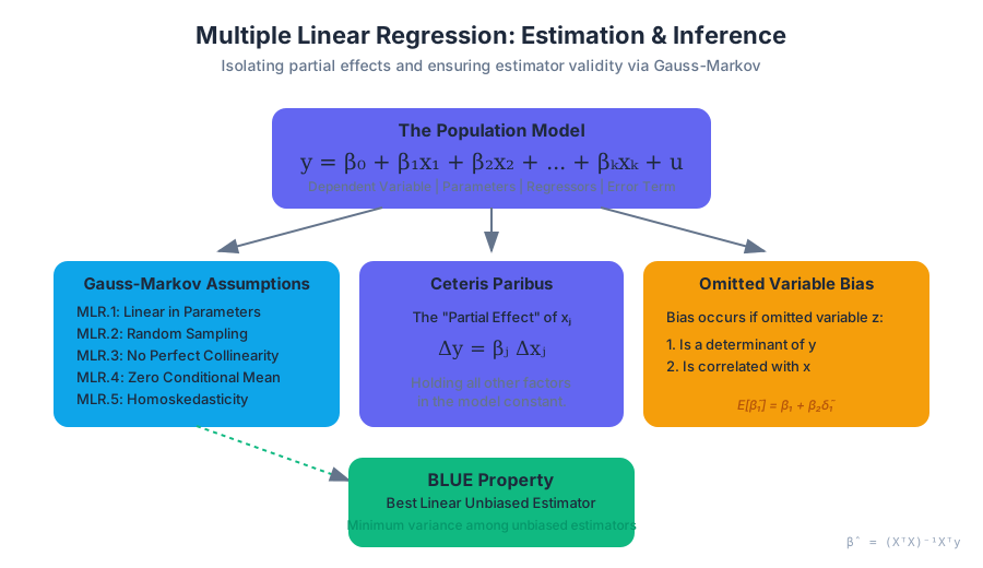
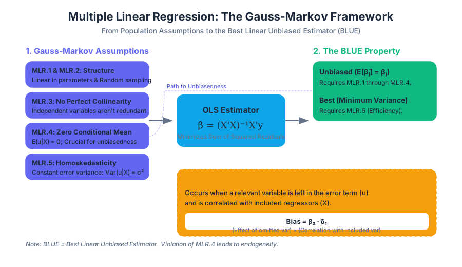
Suppose the "true" population model is: $$y = \beta_0 + \beta_1 x_1 + \beta_2 x_2 + u$$ If we mistakenly estimate a model that excludes $x_2$: $$\tilde{y} = \tilde{\beta}_0 + \tilde{\beta}_1 x_1 + \tilde{u}$$ The estimator $\tilde{\beta}_1$ will generally be biased. The relationship between the biased estimator and the true parameter is: $$E[\tilde{\beta}_1] = \beta_1 + \beta_2 \tilde{\delta}_1$$ where $\tilde{\delta}_1$ is the slope coefficient from a regression of the omitted variable ($x_2$) on the included variable ($x_1$).
Direction of Bias
The direction of the bias depends on the signs of $\beta_2$ (the effect of the omitted variable on $y$) and $Corr(x_1, x_2)$.
| $Corr(x_1, x_2) > 0$ | $Corr(x_1, x_2) < 0$ | |
|---|---|---|
| $\beta_2 > 0$ | Positive Bias (Overestimation) | Negative Bias (Underestimation) |
| $\beta_2 < 0$ | Negative Bias (Underestimation) | Positive Bias (Overestimation) |
Professor's Note: If the omitted variable is uncorrelated with the included regressor ($\tilde{\delta}_1 = 0$), the OLS estimator remains unbiased, though it may be less efficient.
The Gauss-Markov Theorem: Why OLS?
Ordinary Least Squares (OLS) is the most widely used estimation method because, under specific conditions, it possesses ideal statistical properties. These conditions are known as the Gauss-Markov Assumptions.
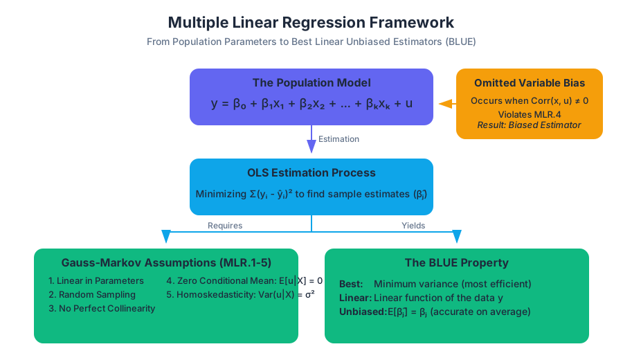
The MLR Assumptions (MLR.1 - MLR.5)
- MLR.1: Linear in Parameters: The model in the population can be written as $y = \beta_0 + \beta_1 x_1 + \dots + \beta_k x_k + u$.
- MLR.2: Random Sampling: We have a random sample of $n$ observations following the population model.
- MLR.3: No Perfect Collinearity: In the sample, none of the independent variables is constant, and there are no exact linear relationships among the independent variables.
- MLR.4: Zero Conditional Mean: The error $u$ has an expected value of zero given any values of the independent variables: $E[u | x_1, \dots, x_k] = 0$.
- MLR.5: Homoskedasticity: The error $u$ has the same variance given any values of the explanatory variables: $Var(u | x_1, \dots, x_k) = \sigma^2$.
The BLUE Property
Theorem: Under assumptions MLR.1 through MLR.5, the OLS estimators $\hat{\beta}_0, \hat{\beta}_1, \dots, \hat{\beta}_k$ are the Best Linear Unbiased Estimators (BLUE).
- Best: Minimum variance (most efficient) among all linear unbiased estimators.
- Linear: The estimator is a linear function of the data ($y$).
- Unbiased: On average, the estimator equals the true population parameter ($E[\hat{\beta}_j] = \beta_j$).
Implementation: OLS via Matrix Algebra
In a professional or computational context, MLR is solved using matrix algebra. This is more efficient than solving $k+1$ simultaneous equations manually.
import numpy as np

def manual_ols(X, y):
    """
    Implements OLS estimation using the Normal Equation:
    beta_hat = (X^T * X)^-1 * X^T * y
    """
    # Add a column of ones to X for the intercept beta_0
    n_obs = X.shape[0]
    X_with_intercept = np.hstack([np.ones((n_obs, 1)), X])

    # Calculate (X^T * X)^-1
    xtx = np.dot(X_with_intercept.T, X_with_intercept)
    xtx_inv = np.linalg.inv(xtx)

    # Calculate X^T * y
    xty = np.dot(X_with_intercept.T, y)

    # Final beta coefficients
    beta_hat = np.dot(xtx_inv, xty)

    # Residuals and Variance Estimation
    residuals = y - np.dot(X_with_intercept, beta_hat)
    dof = n_obs - X_with_intercept.shape[1]
    sigma_squared = np.sum(residuals**2) / dof

    # Variance-Covariance Matrix of coefficients
    var_beta = sigma_squared * xtx_inv
    std_errors = np.sqrt(np.diagonal(var_beta))

    return beta_hat, std_errors

# Example Usage
X_data = np.array([[15, 2], [18, 3], [20, 5], [22, 5], [25, 7]]) # e.g., Education, Experience
y_data = np.array([30, 35, 42, 48, 55]) # e.g., Wage
betas, se = manual_ols(X_data, y_data)
print(f"Coefficients: {betas}")
print(f"Std Errors: {se}")
Statistical Inference: The t-test
Once we have our estimates $\hat{\beta}_j$, we need to determine if they are statistically significant—that is, whether we can confidently say they are different from zero in the population.
The t-statistic
To test the null hypothesis $H_0: \beta_j = 0$ against the alternative $H_1: \beta_j \neq 0$, we calculate the t-statistic: $$t_{\hat{\beta}_j} = \frac{\hat{\beta}_j}{se(\hat{\beta}_j)}$$ Where $se(\hat{\beta}_j)$ is the standard error of the estimator. Under the Classical Linear Model (CLM) assumptions (which add normality of errors to MLR.1-MLR.5), this statistic follows a $t$-distribution with $n - k - 1$ degrees of freedom.
Decision Rules
- p-value approach: If the p-value is less than the significance level $\alpha$ (usually 0.05), reject $H_0$.
- Critical value approach: If $|t| > t_{critical}$, reject $H_0$.
\text{Standard Error of } \hat{\beta}_j: \\
se(\hat{\beta}_j) = \sqrt{\frac{\hat{\sigma}^2}{SST_j(1 - R_j^2)}} \\
\\
\text{where } SST_j \text{ is total variation in } x_j, \\
\text{and } R_j^2 \text{ is the R-squared from regressing } x_j \text{ on all other } x\text{'s.}
Joint Significance: The F-test
Sometimes we want to test multiple hypotheses simultaneously. For example, we might ask: "Do experience and tenure jointly affect wages, even if neither is significant individually?"
Restricted vs. Unrestricted Models
To perform an F-test, we compare two models:
- Unrestricted Model (UR): The full model with all variables.
- Restricted Model (R): The model where the null hypothesis is imposed (e.g., the coefficients of the variables being tested are set to zero).
The F-statistic is calculated as: $$F = \frac{(SSR_r - SSR_{ur}) / q}{SSR_{ur} / (n - k - 1)}$$ Where:
- $SSR_r$ is the Sum of Squared Residuals from the restricted model.
- $SSR_{ur}$ is the Sum of Squared Residuals from the unrestricted model.
- $q$ is the number of restrictions (number of variables being tested).
- $n - k - 1$ is the degrees of freedom of the unrestricted model.
| Feature | t-test | F-test |
|---|---|---|
| Scope | Single coefficient | Multiple coefficients (joint) |
| Hypothesis | $\beta_j = 0$ | $\beta_1 = \beta_2 = \dots = \beta_q = 0$ |
| Distribution | $t_{n-k-1}$ | $F_{q, n-k-1}$ |
| Direction | One-tailed or Two-tailed | Always One-tailed (right-tail) |
Functional Forms: Non-linear Relationships
MLR is "linear in parameters," but the variables themselves can be non-linear. This allows for immense flexibility in modeling.
Logarithmic Transformations
Log transformations are used to model percentage changes (elasticities).
- Log-Log Model: $\log(y) = \beta_0 + \beta_1 \log(x) + u$. $\beta_1$ is the elasticity of $y$ with respect to $x$.
- Log-Linear Model: $\log(y) = \beta_0 + \beta_1 x + u$. $100 \cdot \beta_1$ is the percentage change in $y$ for a one-unit change in $x$.
- Linear-Log Model: $y = \beta_0 + \beta_1 \log(x) + u$. $\beta_1 / 100$ is the change in $y$ for a 1% change in $x$.
Quadratic Forms
To capture "diminishing marginal returns," we use squared terms: $$y = \beta_0 + \beta_1 x + \beta_2 x^2 + u$$ The marginal effect of $x$ is no longer constant: $\frac{\Delta y}{\Delta x} = \beta_1 + 2\beta_2 x$. If $\beta_1 > 0$ and $\beta_2 < 0$, the relationship follows an inverted U-shape.
Real-World Application: Stata Workflow
In practice, researchers use specialized software like Stata to handle these calculations and perform diagnostic tests.
// Load dataset (e.g., wage data)
use "http://www.stata-press.com/data/r15/nlsw88.dta", clear

// 1. Estimate Multiple Regression
// wage: dependent variable
// educ, exper, tenure: independent variables
regress wage educ exper tenure

// 2. Test for Omitted Variable Bias (Ramsey RESET test)
ovtest

// 3. Perform a t-test on a specific coefficient (automatic in 'regress' output)
// But we can also test specific values:
test educ = 1.5

// 4. Perform an F-test for joint significance of exper and tenure
test exper tenure

// 5. Generate a non-linear model (Quadratic experience)
gen exper2 = exper^2
regress wage educ exper exper2 tenure

// 6. Visualizing the partial effect of education
avplot educ
Common Pitfalls and Misconceptions
- Mistaking $R^2$ for Model Quality: A high $R^2$ does not mean the model is "good" or that the estimates are unbiased. It simply means the $x$ variables explain a lot of the variation in $y$. In social sciences, low $R^2$ values (0.1 - 0.3) are very common.
- The "Everything but the Kitchen Sink" Approach: Adding too many variables to avoid OVB can lead to Multicollinearity, which inflates standard errors and makes estimates unstable.
- Correlation vs. Causation: Even with many controls, MLR only establishes causality if the Zero Conditional Mean assumption (MLR.4) holds. If an unobserved factor (like "innate ability") is correlated with both education and wages, the coefficient on education is still biased.
- Interpreting Logs: Forgetting to multiply by 100 when interpreting log-linear models is a frequent student error.
Summary of Inference Logic
The journey from data to insight in MLR follows a strict logical pipeline:
- Specify the model based on economic theory.
- Collect data and ensure it meets the random sampling assumption.
- Estimate coefficients using OLS.
- Check Gauss-Markov assumptions (especially linearity and homoskedasticity).
- Evaluate statistical significance using t-tests for individual variables and F-tests for groups.
- Interpret the magnitude of the coefficients in the context of the units (or logs) used.
Functional Forms and Heteroskedasticity
Key concepts: Log-Log Models · Quadratic Specifications · Heteroskedasticity · Robust Standard Errors · Breusch-Pagan Test
Explores non-linear relationships using logs and quadratics, and addresses violations of the constant variance assumption.
Functional Forms and Heteroskedasticity
In the pursuit of modeling economic phenomena, we often find that the rigid structure of a simple linear relationship—where a one-unit change in $X$ results in a constant $\beta$ change in $Y$—is insufficient. The real world is characterized by diminishing returns, percentage-based growth, and variances that fluctuate alongside the scale of the data. To capture these nuances, the econometrician must master two critical domains: the selection of Functional Forms to capture non-linearities and the treatment of Heteroskedasticity to ensure valid statistical inference.
Non-Linear Functional Forms
While the Ordinary Least Squares (OLS) estimator requires the model to be linear in parameters, it does not require the model to be linear in variables. This distinction is the gateway to modeling complex economic behavior. By transforming variables using logarithms or polynomials, we can model non-linear relationships while remaining within the powerful framework of OLS.
Logarithmic Transformations
Logarithmic models are perhaps the most common non-linear transformations in economics. They are particularly useful when dealing with variables that are strictly positive and have skewed distributions, such as wages, firm size, or population.
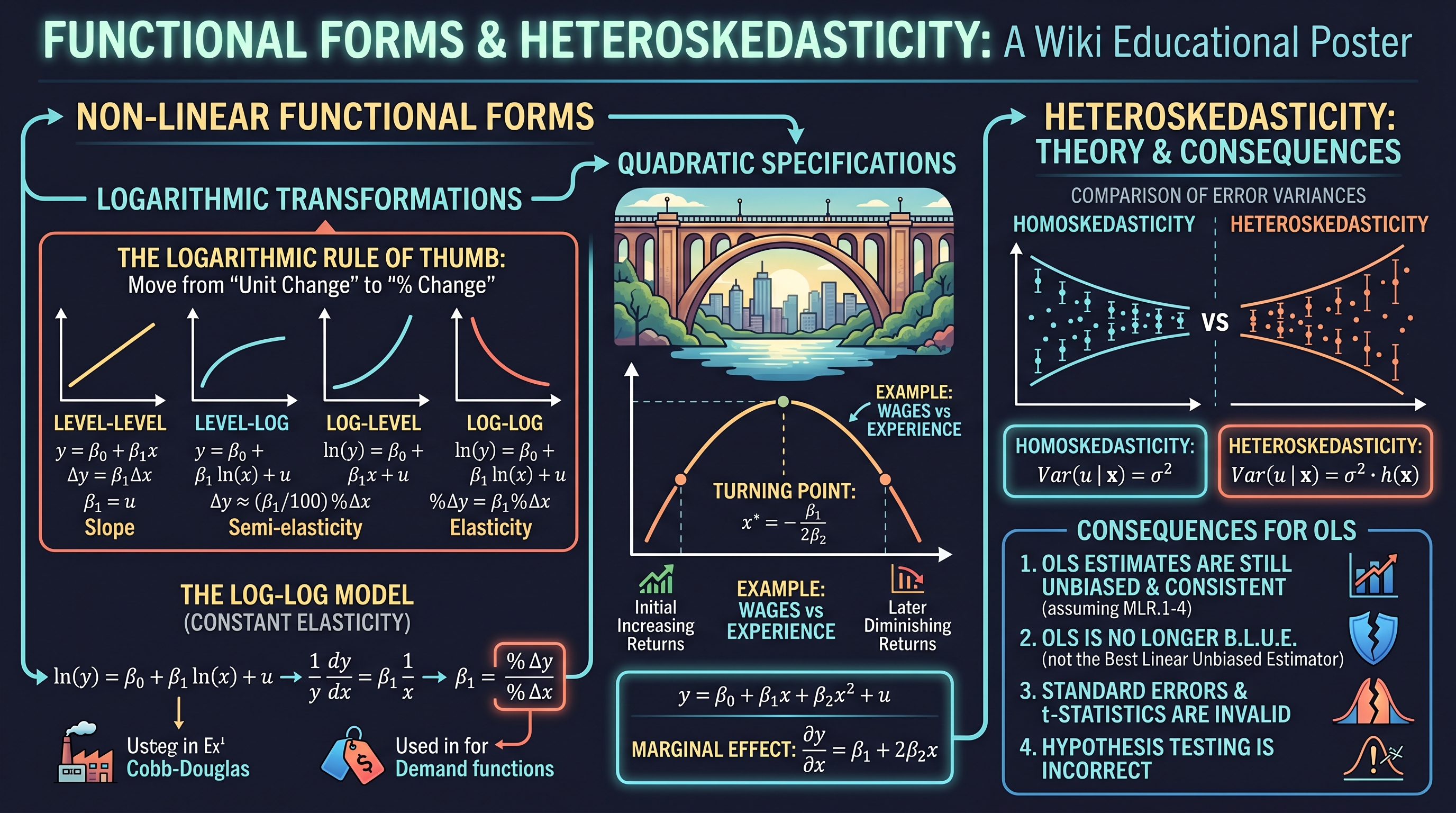
The Logarithmic Rule of Thumb: When a variable is logged, we move from discussing "unit changes" to "percentage changes."
There are three primary logarithmic specifications, each with a distinct interpretation of the slope coefficient $\beta_1$:
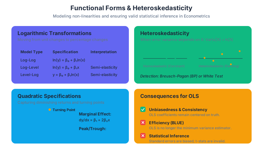
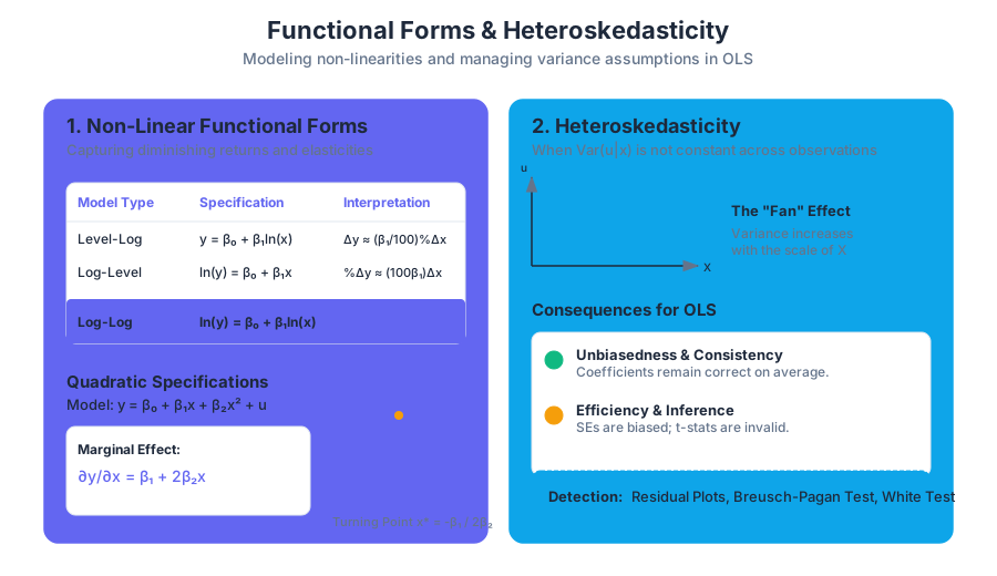
| Model Type | Specification | Interpretation of $\beta_1$ | Name of $\beta_1$ |
|---|---|---|---|
| Level-Level | $y = \beta_0 + \beta_1 x + u$ | $\Delta y = \beta_1 \Delta x$ | Slope |
| Level-Log | $y = \beta_0 + \beta_1 \ln(x) + u$ | $\Delta y \approx (\beta_1 / 100) % \Delta x$ | Semi-elasticity |
| Log-Level | $\ln(y) = \beta_0 + \beta_1 x + u$ | $% \Delta y \approx (100 \cdot \beta_1) \Delta x$ | Semi-elasticity |
| Log-Log | $\ln(y) = \beta_0 + \beta_1 \ln(x) + u$ | $% \Delta y = \beta_1 % \Delta x$ | Elasticity |
The Log-Log Model (Constant Elasticity)
In a Log-Log Model, both the dependent and independent variables are transformed by the natural logarithm. This is the standard specification for estimating demand functions or production functions (like the Cobb-Douglas model).
Mathematical Derivation of Elasticity: Consider the model: $\ln(y) = \beta_0 + \beta_1 \ln(x) + u$. To find the effect of $x$ on $y$, we take the derivative with respect to $x$: $$\frac{d(\ln y)}{dx} = \beta_1 \frac{d(\ln x)}{dx}$$ Using the chain rule ($\frac{d \ln(y)}{dy} = \frac{1}{y}$): $$\frac{1}{y} \cdot \frac{dy}{dx} = \beta_1 \cdot \frac{1}{x}$$ Rearranging for $\beta_1$: $$\beta_1 = \frac{dy/y}{dx/x} = \frac{% \Delta y}{% \Delta x}$$ Thus, $\beta_1$ represents the elasticity of $y$ with respect to $x$.
import numpy as np
import pandas as pd
import statsmodels.api as sm

# Example: Estimating Price Elasticity of Demand
# Generating synthetic data for Quantity (Q) and Price (P)
np.random.seed(42)
price = np.random.uniform(10, 50, 100)
# Demand function: Q = A * P^(-1.5) -> ln(Q) = ln(A) - 1.5*ln(P)
log_q = 10 - 1.5 * np.log(price) + np.random.normal(0, 0.1, 100)

df = pd.DataFrame({'log_price': np.log(price), 'log_quantity': log_q})

# OLS Regression on Log-Log specification
X = sm.add_constant(df['log_price'])
model = sm.OLS(df['log_quantity'], X).fit()

print(f"Estimated Elasticity: {model.params['log_price']:.4f}")
# Output will be close to -1.5
Quadratic Specifications
Quadratic models are used to capture relationships that have a "turning point," representing either diminishing or increasing marginal effects. A classic example is the relationship between Experience and Wages. Initially, an extra year of experience increases wages significantly, but this effect eventually tapers off or even turns negative as skills become obsolete or retirement nears.
The general form is: $$y = \beta_0 + \beta_1 x + \beta_2 x^2 + u$$
To find the marginal effect of $x$ on $y$, we take the partial derivative: $$\frac{\partial y}{\partial x} = \beta_1 + 2\beta_2 x$$
Insight: The effect of $x$ on $y$ is no longer constant; it depends on the starting value of $x$.
Finding the Turning Point: The "peak" or "trough" of the curve occurs where the marginal effect is zero: $$\beta_1 + 2\beta_2 x^* = 0 \implies x^* = -\frac{\beta_1}{2\beta_2}$$
Heteroskedasticity: Theory and Consequences
In the standard Gauss-Markov framework, we assume Homoskedasticity (Assumption MLR.5): the variance of the error term $u$, conditional on the explanatory variables, is constant. $$Var(u | x_1, x_2, ..., x_k) = \sigma^2$$
Heteroskedasticity occurs when this assumption is violated, meaning the variance of the unobservables changes across different levels of the independent variables: $$Var(u | \mathbf{x}) = h(\mathbf{x})$$
Why Heteroskedasticity Matters
It is a common misconception that heteroskedasticity biases the OLS coefficients. This is false.
| Property | Impact of Heteroskedasticity |
|---|---|
| Unbiasedness | No Impact. OLS remains unbiased (MLR.1 - MLR.4 still hold). |
| Consistency | No Impact. OLS remains consistent as $n \to \infty$. |
| Efficiency | Lost. OLS is no longer the Best Linear Unbiased Estimator (BLUE). |
| Standard Errors | Invalid. The usual OLS standard error formulas are biased. |
| Inference | Invalid. $t$-statistics and $F$-statistics no longer follow the $t$ and $F$ distributions. |
Detecting Heteroskedasticity
Before correcting for heteroskedasticity, we must confirm its presence. While visual inspection of residual plots is a good first step, formal statistical tests provide more rigor.
The Breusch-Pagan (BP) Test
The BP test checks if the variance of the error depends on the explanatory variables in a linear way.
- Estimate the OLS model: $y = \beta_0 + \beta_1 x_1 + ... + \beta_k x_k + u$.
- Obtain the squared residuals: $\hat{u}^2$.
- Run the auxiliary regression: $\hat{u}^2 = \delta_0 + \delta_1 x_1 + ... + \delta_k x_k + v$.
- Test the Null Hypothesis: $H_0: \delta_1 = \delta_2 = ... = \delta_k = 0$.
- Compute the statistic: $LM = n \cdot R^2_{\hat{u}^2}$, which follows a $\chi^2_k$ distribution.
The White Test
The White test is more general than the BP test because it allows for non-linearities in the variance (by including squares and cross-products of the regressors). However, it consumes many degrees of freedom if there are many $X$ variables.
\text{White Test Auxiliary Regression:} \\
\hat{u}^2 = \delta_0 + \delta_1 x_1 + \delta_2 x_2 + \delta_3 x_1^2 + \delta_4 x_2^2 + \delta_5 (x_1 x_2) + v
Correcting for Heteroskedasticity
Once heteroskedasticity is detected, we have two primary paths: Robust Inference (adjusting the standard errors) or Weighted Least Squares (transforming the model).
Heteroskedasticity-Robust Standard Errors
The most common modern approach is to use Robust Standard Errors (also known as White, Huber, or Eicker standard errors). This method allows us to keep the OLS estimates but adjusts the standard errors to be valid even when the variance is non-constant.
The robust variance estimator for $\hat{\beta}_j$ in a simple regression is: $$\widehat{Var}(\hat{\beta}_1) = \frac{\sum (x_i - \bar{x})^2 \hat{u}_i^2}{SST_x^2}$$
In matrix notation, this is often called the Sandwich Estimator: $$\hat{V}_{robust} = (X'X)^{-1} (X' \hat{\Omega} X) (X'X)^{-1}$$ where $\hat{\Omega}$ is a diagonal matrix of squared residuals.
Weighted Least Squares (WLS)
If we know the exact form of the heteroskedasticity (i.e., $Var(u|x) = \sigma^2 h(x)$), WLS is more efficient than OLS. We "weight" the observations by $1/\sqrt{h(x)}$, effectively giving more importance to observations with lower variance.
Steps for WLS:
- Assume $Var(u|x) = \sigma^2 x_i$.
- Divide the entire regression equation by $\sqrt{x_i}$.
- The transformed error term will now be homoskedastic.
Implementation and Real-World Usage
In professional practice, researchers rarely rely on the assumption of homoskedasticity. The "gold standard" in applied econometrics is to report robust standard errors by default.
// Stata Example: Wage Equation with Functional Forms and Robust SEs

// 1. Load dataset
use "http://www.stata.com/data/jmulti/wage1.dta", clear

// 2. Estimate a Log-Level model with a Quadratic term for Experience
// Model: log(wage) = b0 + b1*educ + b2*exper + b3*exper^2 + u
gen exper_sq = exper^2
reg lwage educ exper exper_sq, robust

// 3. Post-estimation: Find the turning point for experience
// Turning point = -b[exper] / (2 * b[exper_sq])
scalar tp = -_b[exper] / (2 * _b[exper_sq])
display "The wage-maximizing years of experience is: " tp

// 4. Test for Heteroskedasticity (Breusch-Pagan)
// Note: estat hettest usually follows a standard reg (non-robust)
reg lwage educ exper exper_sq
estat hettest
Common Pitfalls and Misconceptions
- Logging Zero or Negative Values: The natural log is only defined for $x > 0$. If your data contains zeros (e.g., years of education), researchers often use $\ln(x + 1)$, though this can slightly alter interpretation.
- Interpreting Log-Level as Percentages: Remember that for a coefficient $\beta = 0.10$ in a log-level model, the effect is a $10%$ increase, not a $0.10%$ increase. However, for large $\beta$, the approximation $% \Delta y \approx 100 \cdot \beta$ breaks down, and one should use $100 \cdot (e^\beta - 1)$.
- Robust SEs are not a Panacea: While robust standard errors fix inference for heteroskedasticity, they do not fix bias caused by omitted variables, measurement error, or endogeneity.
- The "Robust" Trade-off: In very small samples, robust standard errors can be less reliable than standard OLS errors if the homoskedasticity assumption actually holds.
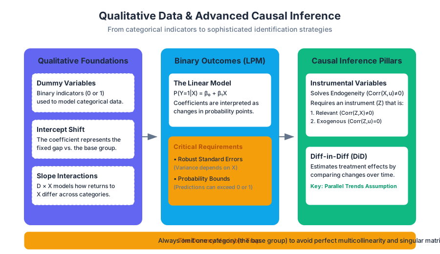
Qualitative Data and Advanced Causal Inference
Key concepts: Dummy Variable Trap · Linear Probability Model (LPM) · Instrumental Variables (IV) · Difference-in-Differences (DiD)
Introduces dummy variables for categorical data and advanced methods for identifying causal effects in the presence of endogeneity.
Qualitative Data and Advanced Causal Inference
In the rigorous pursuit of economic truth, we often find that the most compelling questions involve variables that cannot be measured on a continuous scale—gender, race, employment status, or the presence of a specific policy. Furthermore, the "gold standard" of experimental design is rarely available to social scientists. We are frequently left with observational data where the variables of interest are endogenous, meaning they are correlated with the very error terms we hope to minimize.
This section explores the transition from simple linear models to sophisticated causal frameworks. We begin by formalizing the treatment of qualitative information through dummy variables, navigate the pitfalls of the Linear Probability Model, and conclude with the pillars of modern causal inference: Instrumental Variables (IV) and Difference-in-Differences (DiD).
Qualitative Information and Dummy Variables
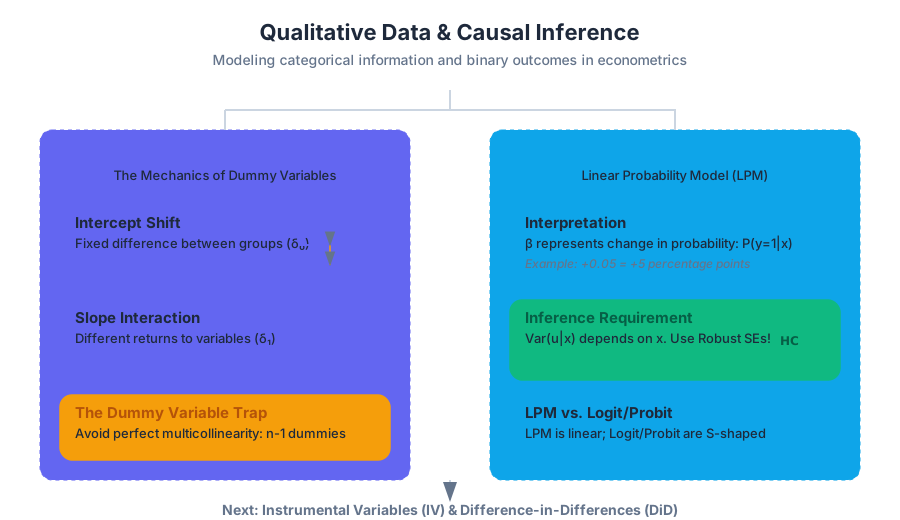
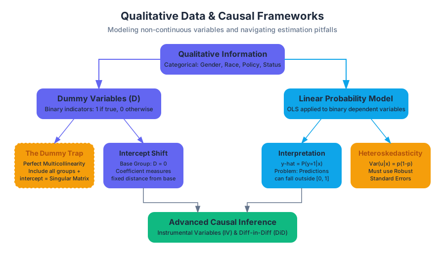
In standard regression, we assume variables like income or distance are continuous. However, much of human experience is categorical. To incorporate this into a linear framework, we use Dummy Variables (also known as binary or indicator variables).
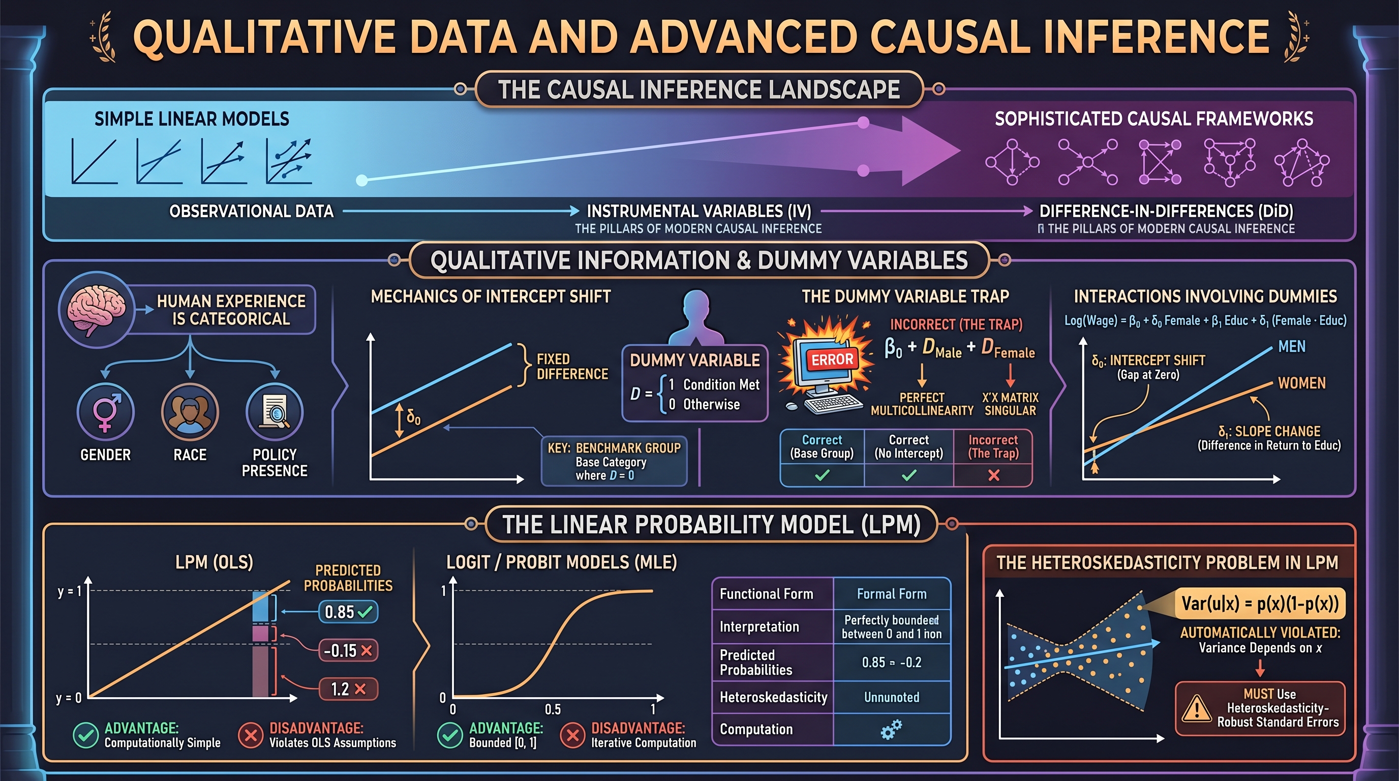
A dummy variable $D$ is defined as: $$D = \begin{cases} 1 & \text{if the condition is met} \ 0 & \text{otherwise} \end{cases}$$
The Mechanics of the Intercept Shift
When we include a dummy variable in a regression, such as $Wage = \beta_0 + \delta_0 Female + \beta_1 Exper + u$, the coefficient $\delta_0$ represents a fixed difference in the intercept between the two groups.
Definition: The Benchmark Group In any model containing dummy variables, the group for which the dummy is 0 is referred to as the base group, benchmark group, or omitted category. All dummy coefficients are interpreted as the expected difference relative to this base group, ceteris paribus.
The Dummy Variable Trap
A common error for novice econometricians is attempting to include a dummy variable for every possible category in a set while also retaining the intercept. This leads to perfect multicollinearity.
If you have two categories (e.g., Male and Female) and you include $D_{male}$, $D_{female}$, and an intercept $\beta_0$, the model cannot be estimated. This is because $D_{male} + D_{female} = 1$ for every observation, which is exactly equal to the constant associated with the intercept. The matrix $X'X$ becomes singular and non-invertible.
| Strategy | Specification | Result |
|---|---|---|
| Correct (Base Group) | $Y = \beta_0 + \beta_1 D_1 + u$ | $\beta_0$ is the mean of group 0; $\beta_1$ is the difference. |
| Correct (No Intercept) | $Y = \alpha_1 D_0 + \alpha_2 D_1 + u$ | $\alpha_1$ and $\alpha_2$ are the absolute means of each group. |
| Incorrect (The Trap) | $Y = \beta_0 + \beta_1 D_0 + \beta_2 D_1 + u$ | Failure: Perfect multicollinearity; Stata/R will drop one variable. |
Interactions Involving Dummies
We can also model differences in slopes by interacting a dummy with a continuous variable. $$Log(Wage) = \beta_0 + \delta_0 Female + \beta_1 Educ + \delta_1 (Female \cdot Educ) + u$$ In this case:
- $\delta_0$ is the "gender gap" for someone with zero education.
- $\delta_1$ is the difference in the return to education between men and women.
The Linear Probability Model (LPM)
When the dependent variable ($y$) is binary, we enter the realm of discrete choice modeling. The simplest approach is the Linear Probability Model (LPM), where we use OLS to estimate a binary outcome.
Interpretation
In an LPM, the predicted value $\hat{y}$ is interpreted as the probability that $y=1$ given the values of $x$. $$P(y=1|x) = \beta_0 + \beta_1 x_1 + \dots + \beta_k x_k$$ The coefficient $\beta_j$ represents the change in the probability of the event occurring for a one-unit increase in $x_j$, holding other factors constant.
Advantages and Disadvantages
While computationally simple and highly interpretable, the LPM violates several standard OLS assumptions.
| Feature | Linear Probability Model (LPM) | Logit / Probit Models |
|---|---|---|
| Functional Form | Linear: $x\beta$ | Non-linear: $\Lambda(x\beta)$ or $\Phi(x\beta)$ |
| Interpretation | Marginal effect is constant ($\beta$) | Marginal effect depends on $x$ |
| Predicted Probabilities | Can be $<0$ or $>1$ (nonsensical) | Strictly bounded between 0 and 1 |
| Heteroskedasticity | Always present by construction | Handled via Maximum Likelihood |
| Computation | OLS (Fast, closed-form) | Iterative (Slower) |
The Heteroskedasticity Problem in LPM
In a binary model, the variance of the error term $u$ is $Var(u|x) = p(x)(1-p(x))$, where $p(x)$ is the probability of success. Since this variance depends on $x$, the Gauss-Markov assumption of homoskedasticity is automatically violated.
Critical Insight: To obtain valid inference (t-stats and p-values) in an LPM, you must use heteroskedasticity-robust standard errors.
# Low-level implementation of LPM with Robust Standard Errors
import numpy as np
import pandas as pd

def estimate_lpm_robust(X, y):
    """
    Estimates a Linear Probability Model with White's Robust Standard Errors.
    X: Design matrix (including intercept)
    y: Binary dependent variable
    """
    # 1. OLS Coefficients: beta = (X'X)^-1 X'y
    xtx_inv = np.linalg.inv(X.T @ X)
    beta = xtx_inv @ X.T @ y

    # 2. Residuals
    y_hat = X @ beta
    residuals = y - y_hat

    # 3. Robust Covariance Matrix (HC1)
    # Sigma = (X'X)^-1 * (sum of e_i^2 * x_i * x_i') * (X'X)^-1
    n, k = X.shape
    meat = np.zeros((k, k))
    for i in range(n):
        row = X[i, :].reshape(1, -1)
        meat += (residuals[i]**2) * (row.T @ row)

    # Degrees of freedom adjustment (n / (n-k))
    df_adj = n / (n - k)
    vcov = df_adj * (xtx_inv @ meat @ xtx_inv)

    se = np.sqrt(np.diag(vcov))
    return beta, se

# Example usage with synthetic data
# X = [1, educ, exper], y = employed (0 or 1)
Instrumental Variables (IV) and 2SLS
One of the most profound challenges in econometrics is Endogeneity. This occurs when $Cov(x, u) \neq 0$, violating the Zero Conditional Mean assumption (MLR.4). This usually stems from:
- Omitted Variable Bias (e.g., "Ability" affecting both education and wages).
- Measurement Error in the independent variable.
- Simultaneity (e.g., Supply and Demand).
The IV Solution
To solve this, we find an Instrumental Variable ($z$) that satisfies two conditions:
- Instrument Relevance: $Cov(z, x) \neq 0$. The instrument must be correlated with the endogenous regressor.
- Exclusion Restriction (Instrument Exogeneity): $Cov(z, u) = 0$. The instrument must have no direct effect on $y$ and must not be correlated with other unobserved factors.
Two-Stage Least Squares (2SLS)
The standard method for implementing IV is 2SLS.
\text{Step 1: The First Stage}
\\ \text{Regress the endogenous variable } x \text{ on the instrument } z \text{ and all other exogenous variables } w.
\\ x = \pi_0 + \pi_1 z + \pi_2 w + v
\\ \text{Obtain the predicted values: } \hat{x}

\\ \text{Step 2: The Second Stage}
\\ \text{Regress the dependent variable } y \text{ on the predicted values } \hat{x} \text{ and exogenous variables } w.
\\ y = \beta_0 + \beta_1 \hat{x} + \beta_2 w + u
The intuition is that $\hat{x}$ contains only the "clean" variation in $x$ (the part triggered by $z$), which is uncorrelated with $u$.
Derivation of the IV Estimator
In a simple model $y = \beta_0 + \beta_1 x + u$ with instrument $z$: $$Cov(z, y) = Cov(z, \beta_0 + \beta_1 x + u)$$ $$Cov(z, y) = \beta_1 Cov(z, x) + Cov(z, u)$$ Since $Cov(z, u) = 0$ by assumption: $$\beta_{1, IV} = \frac{Cov(z, y)}{Cov(z, x)}$$
| Metric | OLS Estimator | IV Estimator |
|---|---|---|
| Consistency | Inconsistent if $Cov(x, u) \neq 0$ | Consistent if $z$ is valid |
| Efficiency | More efficient (smaller variance) | Less efficient (larger variance) |
| Bias | Biased in small samples | Biased in small samples (but consistent) |
| Requirement | $E[u | x] = 0$ |
Common Pitfalls: Weak Instruments
If $Cov(z, x)$ is very small, the instrument is "weak." A weak instrument leads to large standard errors and can actually amplify the bias of OLS if the exclusion restriction is even slightly violated. A common rule of thumb is that the F-statistic from the first-stage regression should be greater than 10.
Difference-in-Differences (DiD)
Difference-in-Differences is a quasi-experimental technique used to estimate the causal effect of a specific intervention or policy change. It mimics a randomized control trial by comparing the changes in outcomes over time between a "treatment" group and a "control" group.
The Logic of DiD
Imagine a state increases its minimum wage (Treatment), while a neighboring state does not (Control). We cannot simply compare the treatment group before and after, because other things might have changed over time (e.g., a national recession). We cannot simply compare the two states after the change, because they might have been different to begin with.
DiD calculates the "difference of the differences":
- Difference 1: Change in the treatment group $(Y_{T, post} - Y_{T, pre})$.
- Difference 2: Change in the control group $(Y_{C, post} - Y_{C, pre})$.
- DiD Estimate: $(Y_{T, post} - Y_{T, pre}) - (Y_{C, post} - Y_{C, pre})$.
The Regression Specification
The DiD estimate is easily obtained using an interaction term: $$Y_{it} = \beta_0 + \beta_1 Treat_i + \beta_2 Post_t + \delta (Treat_i \cdot Post_t) + \epsilon_{it}$$
- $Treat_i$: Dummy for being in the treatment group.
- $Post_t$: Dummy for the period after the intervention.
- $\delta$: The DiD coefficient, representing the causal effect of the treatment.
| Group | Pre-Treatment | Post-Treatment | Difference |
|---|---|---|---|
| Control | $\beta_0$ | $\beta_0 + \beta_2$ | $\beta_2$ |
| Treatment | $\beta_0 + \beta_1$ | $\beta_0 + \beta_1 + \beta_2 + \delta$ | $\beta_2 + \delta$ |
| Diff-in-Diff | $\delta$ |
The Parallel Trends Assumption
The validity of DiD rests entirely on the Parallel Trends Assumption: in the absence of the treatment, the difference between the treatment and control groups would have remained constant over time.
Warning: If the treatment group was already trending upward faster than the control group before the policy change, the DiD estimate will be biased upward, falsely attributing the pre-existing trend to the policy.
// Real-world usage in Stata: Card & Krueger (1994) style
// y = employment, state = (1 for NJ, 0 for PA), time = (1 for post-wage hike)

// 1. Basic DiD using interaction syntax
reg employment i.state##i.time, vce(robust)

// 2. The coefficient on the interaction (1.state#1.time) is the DiD effect

// 3. Testing for Parallel Trends (Placebo Test)
// Use data from periods BEFORE the actual treatment
reg employment i.state##i.pre_period_dummy if time == 0, vce(robust)
// If the interaction is significant here, parallel trends is violated.
Summary of Advanced Causal Methods
Choosing the right tool depends on the nature of your data and the source of endogeneity.
| Method | Best Used When... | Key Requirement |
|---|---|---|
| LPM | $Y$ is binary and interpretability is key. | Robust standard errors. |
| IV / 2SLS | $X$ is endogenous (e.g., choice-based). | A valid, strong instrument ($z$). |
| DiD | There is a clear "event" or policy change. | Parallel trends assumption. |
| Fixed Effects | You have panel data (repeated observations). | Endogeneity is constant over time. |
Extended Study: The Wald Estimator
For a binary instrument and binary treatment, the IV estimator simplifies to the Wald Estimator: $$\beta_{Wald} = \frac{E[y|z=1] - E[y|z=0]}{E[x|z=1] - E[x|z=0]}$$ This is essentially the ratio of the "Intent-to-Treat" (ITT) effect to the "compliance rate." It serves as a foundational bridge between the experimental literature and structural econometrics. When you hear a researcher discuss "Local Average Treatment Effects" (LATE), they are referring to the effect of the treatment specifically on the "compliers"—those whose behavior was actually changed by the instrument.
Applied Econometrics with Stata
Key concepts: Do-files · Data Importing · Variable Transformation · Scatterplots · Virtual Computer Lab (VCL)
Practical guide to using Stata for data cleaning, visualization, and regression analysis within a virtual environment.
Applied Econometrics with Stata
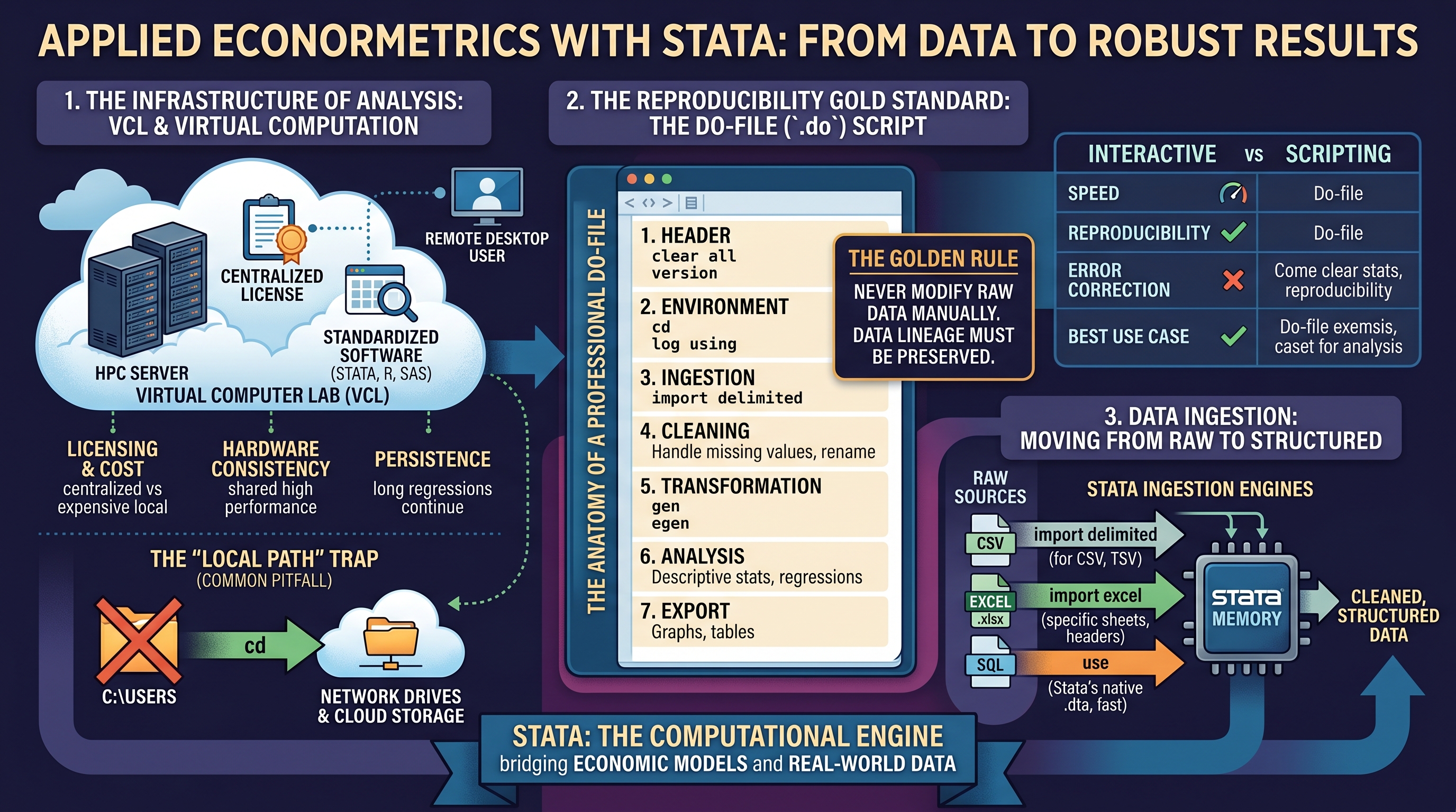
Applied econometrics is the bridge between theoretical economic models and real-world data. While the theory provides the structural equations, Stata serves as the computational engine used to estimate parameters, test hypotheses, and validate assumptions. In a modern research workflow, Stata is not merely a calculator but a comprehensive environment for data management, statistical analysis, and reproducible research.
The Infrastructure of Analysis: Virtual Computer Lab (VCL)
Before a single line of code is written, the researcher must access the computational resources required for heavy lifting. In many academic and professional settings, this is facilitated through a Virtual Computer Lab (VCL).
What it is
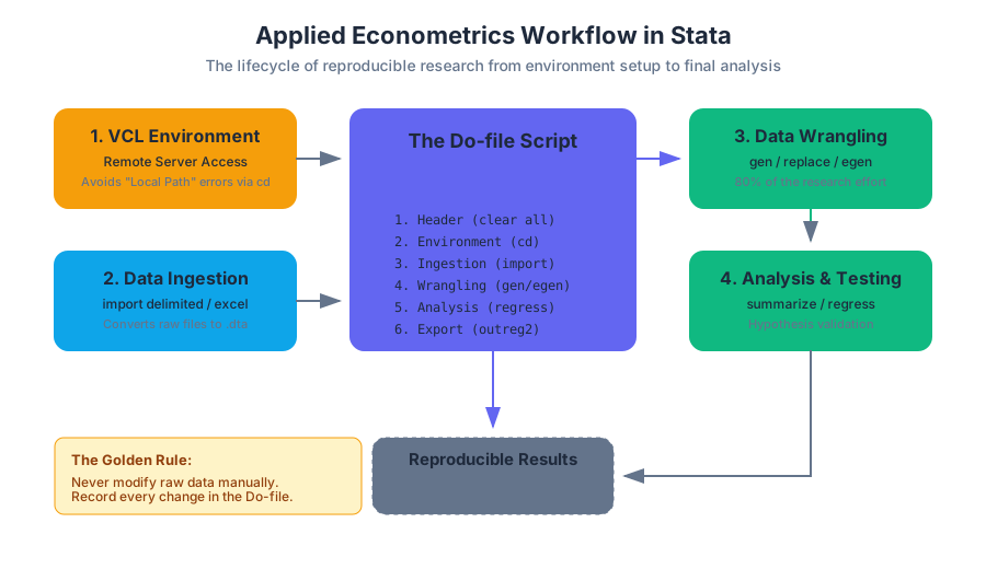
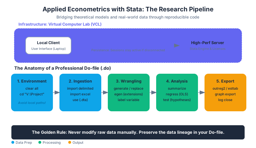
A Virtual Computer Lab (VCL) is a remote-access environment that provides users with a standardized suite of software (like Stata, R, or SAS) without requiring local installation. It operates on a client-server model where the heavy computation occurs on a high-performance server, while the user interacts via a remote desktop protocol.
Why it matters
The VCL solves three critical problems:
- Licensing and Cost: Stata licenses can be prohibitively expensive for individual students; the VCL centralizes this cost.
- Hardware Consistency: It ensures that every student is working with the same processing power and memory, preventing "it works on my machine" errors during large-scale data joins.
- Persistence: Research sessions can often be "disconnected" rather than "logged out," allowing long-running regressions to continue executing even if the user's local laptop loses internet connectivity.
Common Pitfalls: The "Local Path" Trap
A frequent error in the VCL environment is the mismanagement of file paths. Because the VCL is a remote machine, it has its own file system. Users often try to reference files on their local C:\Users\Documents folder, which the VCL cannot see. Researchers must use the cd (change directory) command to point Stata toward the VCL’s network drives or cloud-mapped storage.
The Gold Standard: Do-files and Reproducibility
In econometrics, the result is only as good as the path taken to reach it. Reproducibility is the requirement that an independent researcher can take your raw data and code and produce the exact same results.
What it is
A Do-file (.do) is a plain-text script containing a sequence of Stata commands. Instead of typing commands one-by-one into the "Command" window (interactive mode), the researcher writes the entire pipeline in the Do-file editor and executes it in one go.
The Anatomy of a Professional Do-file
A robust Do-file follows a specific structural hierarchy:
- Header: Version control, memory clearing (
clear all), and logging (log using). - Environment: Setting the working directory (
cd). - Ingestion: Importing raw data.
- Cleaning: Handling missing values, renaming variables, and labeling.
- Transformation: Creating new variables (
gen,egen). - Analysis: Descriptive statistics and regressions.
- Export: Saving results to tables or graphs.
The Golden Rule of Do-files: Never modify your raw data manually. Every change—from dropping an outlier to renaming a column—must be recorded in the Do-file so the "data lineage" is preserved.
| Feature | Interactive Command Window | Do-file Scripting |
|---|---|---|
| Speed | Fast for quick checks | Slower to set up |
| Reproducibility | Zero; history is lost on exit | High; permanent record |
| Error Correction | Must re-type everything | Edit one line and re-run |
| Complexity | Limited to simple tasks | Handles multi-stage pipelines |
| Best Use Case | Browsing data (br) |
Final analysis and HW submissions |
Data Ingestion: Moving from Raw to Structured
Data rarely arrives in Stata's native .dta format. It usually exists as CSVs, Excel spreadsheets, or SQL exports.
Importing Mechanics
Stata provides several engines for data ingestion. The choice depends on the source format and the presence of metadata (like column headers).
import delimited: The modern standard for CSV and text files. It is highly flexible and automatically detects delimiters (commas, tabs, semicolons).import excel: Specifically designed for.xlsxfiles. It allows the researcher to specify which sheet to load and whether the first row contains variable names.use: Used exclusively for Stata's proprietary.dtafiles. It is the fastest method because the data is already structured for Stata's memory.
Implementation Example: The Ingestion Pipeline
// 1. Low-level implementation of a data setup script
capture log close               // Close any open logs
log using "analysis_log.txt", replace

clear all                       // Clear memory
set more off                    // Prevent "more" prompts

// Set the working directory (VCL specific path example)
cd "V:\Economics\Project1"

// Import raw CSV data
import delimited "raw_census_data.csv", case(lower) clear

// Basic data audit
describe                        // Check variable types
summarize                       // Check for impossible values (e.g., age = -1)
list in 1/10                    // Peek at the first 10 observations
Variable Transformation and Data Wrangling
Once data is loaded, it is rarely ready for regression. Econometricians spend roughly 80% of their time in the Data Wrangling phase—transforming raw inputs into theoretically sound variables.
The generate vs. replace Logic
generate(orgen): Creates a brand new variable in the dataset.replace: Modifies the values of an existing variable.egen(Extensions to Generate): Used for complex transformations like calculating means across groups or creating standardized scores (z-scores).
Dummy Variables (Indicator Variables)
A dummy variable is a binary variable that takes the value 1 if a condition is true and 0 otherwise. These are crucial for modeling qualitative differences (e.g., Gender, Treatment vs. Control, or Regional effects).
Mathematical Derivation of Variable Transformation
In a multiple linear regression, we often transform variables to satisfy the Gauss-Markov assumptions or to model non-linear relationships. For example, the Log-Log model is used to estimate elasticities.
\begin{aligned}
\text{Raw Model:} & \quad Y = \beta_0 X^{\beta_1} e^u \\
\text{Transformation:} & \quad \ln(Y) = \ln(\beta_0) + \beta_1 \ln(X) + u \\
\text{Stata Logic:} & \quad \text{gen ln_y = ln(y)} \\
& \quad \text{gen ln_x = ln(x)} \\
& \quad \text{reg ln_y ln_x}
\end{aligned}
Table: Common Transformation Patterns
| Goal | Stata Command | Economic Interpretation |
|---|---|---|
| Interaction | gen x1_x2 = x1 * x2 |
How the effect of $x_1$ changes with $x_2$ |
| Quadratic | gen x_sq = x^2 |
Modeling U-shaped or Diminishing returns |
| Binary | gen treated = (income > 50000) |
Creating a threshold-based group |
| Group Mean | egen avg_inc = mean(inc), by(state) |
Comparing individuals to their peers |
Exploratory Data Analysis (EDA) with Scatterplots
Before running a regression, one must "look" at the data. Visual inspection can reveal outliers, non-linearity, or heteroskedasticity that summary statistics might hide.
The twoway scatter Command
The scatterplot is the primary tool for visualizing the relationship between two continuous variables. In Stata, the twoway command allows for layering, such as plotting a scatterplot and an OLS regression line (the "best fit" line) simultaneously.
Implementation: Visualizing the Relationship
# Third code block: CLI/Shell-style representation of a Stata batch run
# This demonstrates how a researcher might run a script from the terminal
# to generate a plot without opening the GUI.

stata-mp -b do "visualize_returns_to_schooling.do"

# Inside the .do file:
# twoway (scatter wage educ) (lfit wage educ), ///
#        title("Returns to Education") ///
#        xtitle("Years of Schooling") ytitle("Hourly Wage") ///
#        note("Source: 2023 Labor Survey")
# graph export "output_plot.png", replace
Why Scatterplots Matter
- Outlier Detection: A single data point (e.g., a billionaire in a poverty study) can pull the OLS line away from the true trend.
- Heteroskedasticity: If the "spread" of the dots increases as $X$ increases (a fan shape), the standard errors are likely biased, necessitating the
robustcommand. - Non-linearity: If the dots form a curve, a simple linear model (
reg y x) is misspecified.
Advanced Modeling: IV and Difference-in-Differences
As highlighted in the Homework 5 solutions and final exam preparation, applied econometrics moves beyond simple OLS to address Endogeneity and Causal Inference.
Instrumental Variables (IV)
When an explanatory variable $X$ is correlated with the error term $u$ (due to omitted variable bias or simultaneity), OLS is biased. We use an Instrument (Z) that is correlated with $X$ but uncorrelated with $u$.
Stata Syntax: ivregress 2sls y (x = z) w1 w2, robust
Difference-in-Differences (DID)
DID is used to estimate the causal effect of a policy or treatment by comparing the change in outcomes over time between a treatment group and a control group.
The DID Equation: $$Y_{it} = \beta_0 + \beta_1 \text{Treat}_i + \beta_2 \text{Post}_t + \delta(\text{Treat}_i \times \text{Post}t) + \epsilon{it}$$
In Stata, the coefficient of interest ($\delta$) is the interaction term.
Table: Comparison of Regression Estimators
| Method | Command | Use Case | Key Assumption |
|---|---|---|---|
| OLS | reg y x |
Baseline correlation | $E[u\vert x] = 0$ (Exogeneity) |
| Robust OLS | reg y x, robust |
When variance is not constant | Handles Heteroskedasticity |
| IV (2SLS) | ivregress 2sls ... |
Endogenous regressors | Instrument Validity & Relevance |
| Fixed Effects | xtreg y x, fe |
Panel data (repeated obs) | Time-invariant unobservables |
Preparation for the Final Exam: Logistics and Strategy
Based on the instructor's guidance, the final exam is a high-stakes assessment of both theoretical understanding and practical application.
Exam Parameters
- Duration: 2 hours (Note: Adjusted from 3 hours).
- Materials: 4 double-sided sheets of notes and a calculator.
- Focus Areas: Multiple Linear Regression, Dummy Variables, IV, and DID.
Strategic Advice for Applied Questions
- Show Your Work: Partial credit is awarded for the logic of the derivation, even if the final calculation is off.
- Interpret the Coefficients: Don't just find $\beta_1 = 0.5$. Explain that "a one-unit increase in $X$ is associated with a 0.5 unit increase in $Y$, holding all other factors constant."
- Check for Robustness: If a question mentions "non-constant variance," always specify that you would use the
, robustoption in Stata.
Appendix: Troubleshooting Common Stata Errors
| Error Code | Meaning | Solution |
|---|---|---|
| r(601) | File not found | Check your cd and file spelling. |
| r(111) | Variable not found | You likely forgot to gen it or misspelled it. |
| r(103) | Too many variables | Check your regression syntax; you might have a comma in the wrong place. |
| r(2000) | No observations | Your if condition or missing data handling dropped everyone. |
"The most powerful tool in Stata isn't the
regresscommand; it's thehelpcommand. Typinghelp [command]provides the full documentation, syntax, and examples needed to solve almost any implementation hurdle."
Course Assessments and Problem Sets
Key concepts: Stata Output Interpretation · Hypothesis Testing Practice · Model Specification · Problem Set Solutions
Collection of practice exams, homework solutions, and study guides for the midterm and final assessments.
Course Assessments and Problem Sets
In the study of econometrics, the transition from theoretical understanding to empirical mastery occurs within the crucible of assessments and problem sets. These exercises are designed to simulate the workflow of a professional data analyst or academic researcher: cleaning raw data, specifying a model based on economic theory, executing the estimation via software (Stata), and—most crucially—interpreting the results through the lens of causal inference.
Successful navigation of these assessments requires more than just memorizing formulas; it demands a deep intuition for the Gauss-Markov assumptions, the mechanics of Ordinary Least Squares (OLS), and the ability to detect and correct for violations like heteroskedasticity or endogeneity.
The Anatomy of Stata Output Interpretation
The cornerstone of every problem set is the interpretation of the Stata regress output. A standard regression table contains three primary components: the Analysis of Variance (ANOVA) table, the Model Fit section, and the Coefficient Table.
The Coefficient Table
This is the "heart" of the output. For a model $Y = \beta_0 + \beta_1 X_1 + \dots + \beta_k X_k + u$, Stata provides estimates for each $\beta_j$.
| Column | Name | Description | Mathematical Identity |
|---|---|---|---|
| Coef. | Point Estimate | The estimated effect of $X_j$ on $Y$, holding other factors constant. | $\hat{\beta}_j$ |
| Std. Err. | Standard Error | The estimated standard deviation of the sampling distribution of $\hat{\beta}_j$. | $se(\hat{\beta}_j) = \sqrt{\widehat{Var}(\hat{\beta}_j)}$ |
| t | t-statistic | The ratio of the coefficient to its standard error. | $t = \frac{\hat{\beta}_j - 0}{se(\hat{\beta}_j)}$ |
| P>|t| | p-value | The probability of observing a t-stat this extreme if $H_0: \beta_j = 0$ is true. | $P( |
| [95% Conf.] | Confidence Interval | The range of values within which we are 95% confident the true $\beta_j$ lies. | $\hat{\beta}j \pm t{c} \cdot se(\hat{\beta}_j)$ |
Key Insight: A coefficient is only as good as its standard error. A large coefficient with an even larger standard error results in a low t-statistic and a high p-value, meaning we cannot reject the null hypothesis that the variable has no effect.
Model Fit and R-Squared
The $R^2$ value represents the proportion of the total variation in $Y$ that is explained by the independent variables in the model. However, $R^2$ mechanically increases as more variables are added. To account for this, we use the Adjusted R-Squared, which penalizes the addition of unnecessary regressors.
$$ \bar{R}^2 = 1 - (1 - R^2) \frac{n - 1}{n - k - 1} $$
Hypothesis Testing Practice
Problem sets frequently require students to perform manual hypothesis tests to ensure they understand the underlying logic of statistical significance.
The t-test for Individual Significance
To test whether a specific variable $X_j$ has a statistically significant effect on $Y$, we follow a four-step process:
- State the Hypotheses: $H_0: \beta_j = 0$ vs. $H_1: \beta_j \neq 0$.
- Calculate the t-stat: $t = \hat{\beta}_j / se(\hat{\beta}_j)$.
- Find the Critical Value: Look up $t_{c}$ for $n - k - 1$ degrees of freedom at the chosen significance level (usually 5%).
- Make a Decision: If $|t| > t_{c}$, reject $H_0$.
The F-test for Joint Significance
When testing whether a group of variables are all zero (e.g., testing if a set of industry dummy variables matters), we use the F-test. This involves comparing a Restricted Model (without the variables) to an Unrestricted Model (with the variables).
F = \frac{(SSR_r - SSR_{ur}) / q}{SSR_{ur} / (n - k - 1)}
Where $SSR$ is the Sum of Squared Residuals and $q$ is the number of restrictions (the number of variables you are testing).
Model Specification and Functional Forms
One of the most common pitfalls in econometrics is "Level-Level" bias—assuming every relationship is linear. Real-world economic data often requires logarithmic or quadratic transformations to satisfy the Ceteris Paribus condition.
Logarithmic Transformations
The interpretation of $\beta$ changes radically depending on the log-specification:
| Model | Dependent Variable | Independent Variable | Interpretation of $\beta_1$ |
|---|---|---|---|
| Level-Level | $y$ | $x$ | $\Delta y = \beta_1 \Delta x$ (Unit change) |
| Level-Log | $y$ | $\ln(x)$ | $\Delta y \approx (\beta_1 / 100) % \Delta x$ |
| Log-Level | $\ln(y)$ | $x$ | $% \Delta y \approx (100 \cdot \beta_1) \Delta x$ |
| Log-Log | $\ln(y)$ | $\ln(x)$ | $% \Delta y \approx \beta_1 % \Delta x$ (Elasticity) |
Quadratic Forms
To capture diminishing or increasing marginal returns (e.g., the effect of experience on wages), we use a quadratic term: $y = \beta_0 + \beta_1 x + \beta_2 x^2 + u$. The "turning point" where the effect of $x$ on $y$ changes direction is calculated as: $$ x^* = \left| \frac{\beta_1}{2\beta_2} \right| $$
Implementation: Stata Workflow
The following code block demonstrates a typical problem set workflow: importing data, generating new variables, running a regression with robust standard errors, and performing a joint hypothesis test.
// 1. Environment Setup
clear all
set more off
capture log close
log using "ProblemSet_Analysis.log", replace

// 2. Data Ingestion and Cleaning
use "http://www.stata.com/data/j_base/wage.dta", clear
label variable wage "Hourly wage in USD"
gen lwage = ln(wage)
gen exper2 = exper^2

// 3. Model Estimation (Multiple Linear Regression)
// We use the 'robust' option to handle potential heteroskedasticity
reg lwage educ exper exper2 tenure, robust

// 4. Post-Estimation: Testing Joint Significance
// Test if experience and tenure are jointly significant
test exper exper2 tenure

// 5. Visualizing the Fit
predict y_hat, xb
scatter lwage educ || lfit lwage educ, title("Wage vs Education")
graph export "regression_plot.png", replace

log close
Mathematical Derivation: The OLS Estimator
To truly understand why Stata produces the numbers it does, one must look at the derivation of the OLS estimator in matrix form. This is the "low-level" implementation of the regression algorithm.
Given the model: Y = Xβ + u

The Goal: Minimize the Sum of Squared Residuals (SSR)
SSR = u'u = (Y - Xβ)'(Y - Xβ)

Expansion:
SSR = Y'Y - β'X'Y - Y'Xβ + β'X'Xβ
Since β'X'Y is a scalar, it is equal to its transpose Y'Xβ:
SSR = Y'Y - 2β'X'Y + β'X'Xβ

First Order Condition (FOC):
∂SSR / ∂β = -2X'Y + 2X'Xβ = 0

Solving for β:
X'Xβ = X'Y
β_hat = (X'X)^-1 X'Y

This result requires that (X'X) is non-singular (no perfect collinearity).
Advanced Topics: Causal Inference
As the course progresses, problem sets shift from simple correlation to Causal Inference. This involves addressing violations of the Zero Conditional Mean assumption ($E[u|X] = 0$).
1. Instrumental Variables (IV)
When $X$ is correlated with $u$ (endogeneity), OLS is biased. We use an instrument $Z$ that is:
- Relevant: $Cov(Z, X) \neq 0$
- Exogenous: $Cov(Z, u) = 0$
2. Difference-in-Differences (DiD)
Used for policy evaluation. It compares the change in outcomes over time between a treatment group and a control group. $$ \delta_{DiD} = (Y_{T, post} - Y_{T, pre}) - (Y_{C, post} - Y_{C, pre}) $$
3. Linear Probability Model (LPM)
When the dependent variable is binary (0 or 1), OLS is referred to as an LPM. While simple to interpret, it has two major flaws: predicted probabilities can fall outside $[0, 1]$, and the error term is inherently heteroskedastic.
Common Pitfalls in Problem Sets
- The Dummy Variable Trap: Including a dummy variable for every category plus an intercept. This causes perfect multicollinearity.
- Solution: Always omit one category (the "base" group).
- Misinterpreting Log-Models: Forgetting to multiply by 100 when interpreting a log-level model. A $\beta = 0.05$ means a 5% increase, not a 0.05% increase.
- Confusing Correlation with Causation: Claiming that $X$ "causes" $Y$ without verifying the Gauss-Markov assumptions, particularly SLR.4/MLR.4 (Zero Conditional Mean).
- Ignoring Significance: Discussing the magnitude of a coefficient that is not statistically significant. If $p > 0.05$, the effect is effectively zero in the population.
Real-World Usage: Python Replication
In modern industry roles (Data Science/Quant Finance), you may need to replicate Stata results using Python's statsmodels library to integrate with a larger production pipeline.
import pandas as pd
import numpy as np
import statsmodels.api as sm
import statsmodels.formula.api as smf

# Load dataset
url = "https://raw.githubusercontent.com/vincentarelbundock/Rdatasets/master/csv/datasets/cars.csv"
df = pd.read_csv(url)

# 1. Model Specification using Formula API (R-style)
# 'dist ~ speed' means regress distance on speed
model = smf.ols(formula='dist ~ speed', data=df)

# 2. Fit the model with Robust Standard Errors (HC3)
results = model.fit(cov_type='HC3')

# 3. Print the summary (mimics Stata output)
print(results.summary())

# 4. Access specific parameters for downstream logic
beta_speed = results.params['speed']
p_val_speed = results.pvalues['speed']

if p_val_speed < 0.05:
    print(f"Speed is a significant predictor (Beta={beta_speed:.4f})")
else:
    print("No significant relationship found.")
Summary of Gauss-Markov Assumptions
The validity of the OLS results depends entirely on these assumptions.
| Assumption | Name | Violation Consequence |
|---|---|---|
| MLR.1 | Linear in Parameters | Model is misspecified; estimates are meaningless. |
| MLR.2 | Random Sampling | Sample is biased; results don't generalize to population. |
| MLR.3 | No Perfect Collinearity | The matrix $(X'X)$ cannot be inverted; Stata drops variables. |
| MLR.4 | Zero Conditional Mean | Bias. The most critical assumption for causality. |
| MLR.5 | Homoskedasticity | OLS is no longer BLUE; standard errors are wrong. |
| MLR.6 | Normality of Errors | Small sample inference (t-tests) is invalid. |
- Ceteris Paribus: "All else equal." The requirement that other relevant factors are held constant when estimating the effect of $X$ on $Y$.
- Endogeneity: A situation where an independent variable is correlated with the error term, usually due to omitted variable bias.
- BLUE: Best Linear Unbiased Estimator. The property that OLS has the minimum variance among all linear unbiased estimators.
- P-value: The smallest significance level at which the null hypothesis can be rejected.
- Heteroskedasticity: When the variance of the error term is not constant across observations.
- Instrumental Variable: A variable used to provide exogenous variation to an endogenous regressor.
- If you add a variable to a regression and the $R^2$ increases but the Adjusted $R^2$ decreases, what does this tell you about the new variable?
- Why is the "Zero Conditional Mean" assumption (MLR.4) considered the most important for causal inference?
- In a log-log model ($\ln(y) = \beta_0 + \beta_1 \ln(x) + u$), if $\beta_1 = 1.5$, what is the effect of a 10% increase in $x$ on $y$?
- What happens to the t-statistic of a coefficient if the sample size $n$ increases, holding the effect size and variance constant?
- You are running a regression of "Salary" on "Gender" (Male/Female) and "Education". If you include both a
Maledummy and aFemaledummy along with an intercept, what error will Stata return?
Exam Strategy Checklist:
- Coefficient Sign: Does the sign of $\hat{\beta}$ match economic theory? If not, check for Omitted Variable Bias.
- Statistical vs. Economic Significance: A variable can be statistically significant (low p-value) but economically tiny (small coefficient). Always check both.
- Robustness: Always check if your results hold when using
robuststandard errors. - Functional Form: If the scatterplot looks curved, try adding a quadratic term ($x^2$) or using logs.
- Degrees of Freedom: Remember that $df = n - k - 1$. This is crucial for finding the correct critical values for t and F tests.
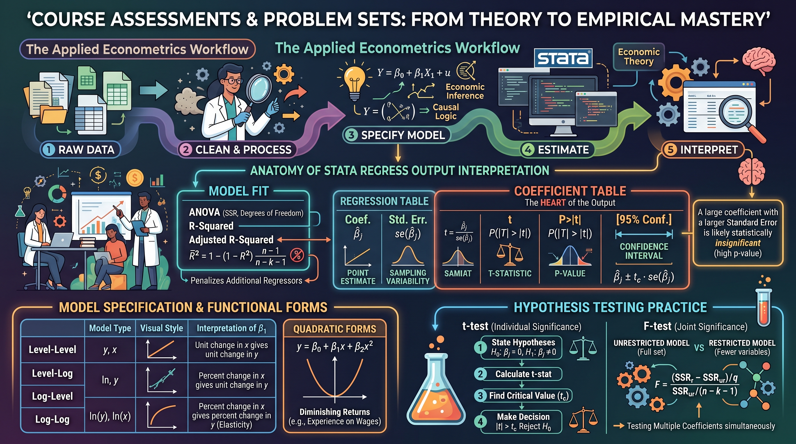
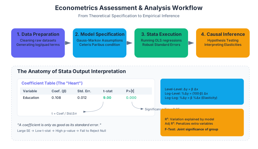
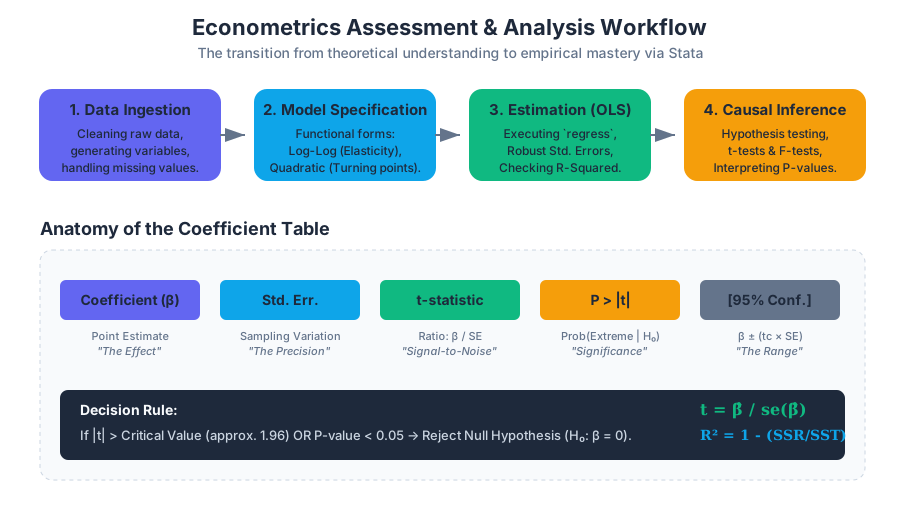
Source Materials
Study Econometric Theory and Empirical Analysis with Stata with AI — Free on Lykke
Sign up for free to generate personalized flashcards, quizzes, and study guides from this course. Chat with an AI tutor that knows the material.
Get Started FreeView this course wiki on Lykke · Browse all public course wikis