Data Structures and Algorithmic Analysis
Institution: MIT
301 study materials · 7 sections
This course provides a comprehensive exploration of fundamental data structures and the algorithms used to manipulate them. Students learn to analyze computational complexity using Big O notation while implementing linear structures like linked lists, stacks, and queues. The curriculum advances into non-linear structures including Binary Search Trees, Balanced Trees, and Directed Graphs, alongside essential sorting and shortest-path algorithms.
Course Sections
Union-Find and Big O Analysis
Key concepts: Big O Notation · Dynamic Connectivity · Quick-Find · Quick-Union · Weighted Quick-Union
Introduction to algorithmic efficiency and the dynamic connectivity problem using Union-Find algorithms.
Union-Find and Big O Analysis
The study of algorithms is inextricably linked to the study of efficiency. In the realm of computer science, we are rarely concerned with whether a problem can be solved—given enough time and memory, most computable problems can be—but rather whether it can be solved within the constraints of reality. This article explores the symbiotic relationship between Big O Analysis, the mathematical language of efficiency, and Union-Find, a sophisticated data structure designed to solve the Dynamic Connectivity problem.
At its core, Union-Find represents a triumph of incremental optimization. By evolving a simple, "eager" approach into a "lazy," weighted, and flattened structure, we can observe a dramatic shift in computational complexity from quadratic time to nearly linear time. This progression serves as a masterclass in algorithmic design and the practical application of asymptotic analysis.
The Foundation: Big O Notation and Complexity Analysis
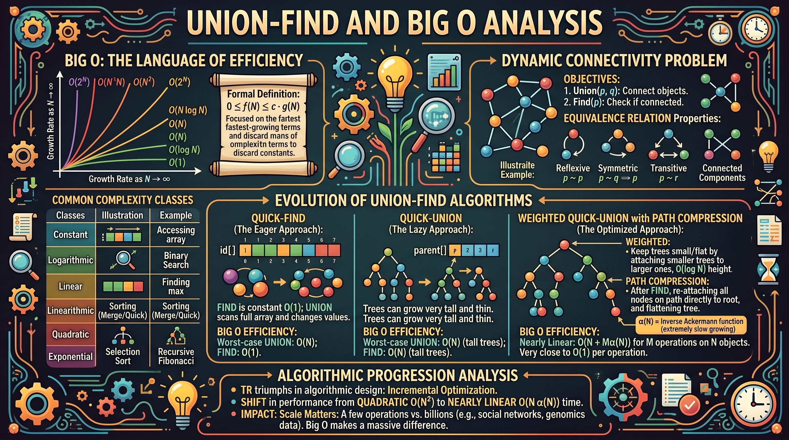
Before diving into specific data structures, we must establish the framework for measurement. Big O Notation provides a theoretical upper bound on the execution time or space requirements of an algorithm as the input size $N$ grows toward infinity. It allows us to ignore hardware-specific constants and focus on the order of growth.
The Formal Definition
Definition: A function $f(N)$ is $O(g(N))$ if there exist positive constants $c$ and $N_0$ such that $0 \le f(N) \le c \cdot g(N)$ for all $N \ge N_0$.
In practice, this means we focus on the fastest-growing term and discard coefficients. For instance, an algorithm that performs $5N^2 + 20N + 100$ operations is categorized as $O(N^2)$. As $N$ becomes massive, the $N^2$ term dominates the total execution time, rendering the $20N$ and constant $100$ negligible.
Common Complexity Classes
| Notation | Name | Description | Example |
|---|---|---|---|
| $O(1)$ | Constant | Time does not change with input size. | Accessing an array index. |
| $O(\log N)$ | Logarithmic | Time increases slowly; doubling $N$ adds a constant step. | Binary Search. |
| $O(N)$ | Linear | Time is directly proportional to input size. | Finding the max in an unsorted list. |
| $O(N \log N)$ | Linearithmic | Slightly worse than linear; standard for efficient sorting. | Merge Sort, Quick Sort. |
| $O(N^2)$ | Quadratic | Time grows with the square of $N$; often involves nested loops. | Selection Sort, Quick-Find Union. |
| $O(2^N)$ | Exponential | Time doubles with each addition to $N$; computationally expensive. | Recursive Fibonacci. |
Why Big O Matters in Union-Find
The Dynamic Connectivity problem involves a set of $N$ objects. We perform $M$ union operations. If our algorithm is $O(N)$, and we do $M$ operations, the total time is $O(MN)$. If $M$ and $N$ are both $10^9$ (a common scale for social networks or genomic data), a quadratic algorithm would take $10^{18}$ operations. On a standard processor, this would take decades. An $O(\log N)$ or $O(\alpha(N))$ algorithm, however, would finish in seconds.
The Dynamic Connectivity Problem
The Union-Find data structure (also known as a Disjoint Set Union or DSU) is designed to solve the dynamic connectivity problem. Given a set of $N$ objects, we need to support two primary operations:
- Union: Connect two objects.
- Find (or Connected): Determine if there is a path connecting two objects.
We assume "connected" is an equivalence relation, meaning it is:
- Reflexive: $p$ is connected to $p$.
- Symmetric: If $p$ is connected to $q$, then $q$ is connected to $p$.
- Transitive: If $p$ is connected to $q$ and $q$ is connected to $r$, then $p$ is connected to $r$.
These properties allow us to partition the objects into connected components. A connected component is a maximal set of objects that are all mutually connected.
Quick-Find: The Eager Approach
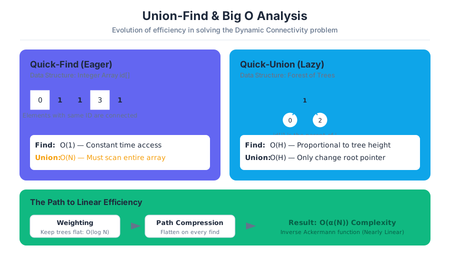
Quick-Find is the most intuitive implementation of Union-Find. It prioritizes the speed of the find operation.
How it Works
We maintain an integer array id[] of size $N$. If id[p] is equal to id[q], then $p$ and $q$ are in the same component.
- Find: Simply check if
id[p] == id[q]. This is a constant time $O(1)$ operation. - Union: To merge components containing $p$ and $q$, we must change all entries whose value is
id[p]toid[q].
Implementation (Java)
public class QuickFindUF {
    private int[] id;

    public QuickFindUF(int N) {
        id = new int[N];
        for (int i = 0; i < N; i++) id[i] = i;
    }

    public boolean connected(int p, int q) {
        return id[p] == id[q];
    }

    public void union(int p, int q) {
        int pid = id[p];
        int qid = id[q];
        for (int i = 0; i < id.length; i++) {
            if (id[i] == pid) id[i] = qid;
        }
    }
}
Analysis of Quick-Find
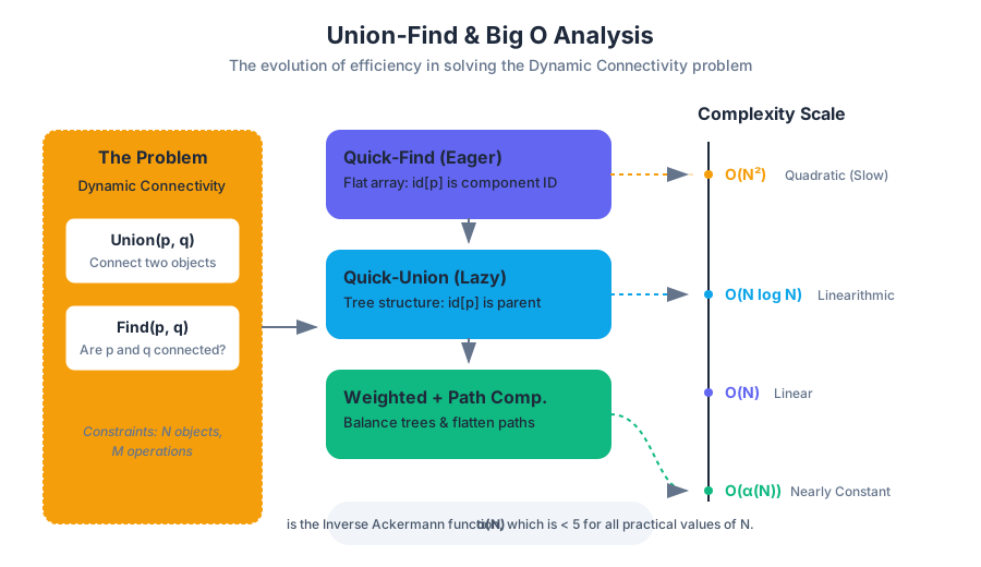
While find is incredibly fast, union is prohibitively expensive. To perform $N$ union operations on $N$ objects, the time complexity is $O(N^2)$.
| Operation | Complexity |
|---|---|
| Initialize | $O(N)$ |
| Union | $O(N)$ |
| Find | $O(1)$ |
The Pitfall: Quick-Find is "eager." It does too much work during the union step to ensure the find step is easy. In a world of Big Data, $O(N^2)$ is effectively non-computable for large $N$.
Quick-Union: The Lazy Approach
To address the $O(N)$ union cost, Quick-Union adopts a "lazy" strategy. Instead of updating every element in a component, we represent components as trees.
How it Works
The id[] array now stores the parent of each element.
- Find: To find the component of $p$, follow parent pointers until you reach a root (where
id[i] == i). - Union: To merge components containing $p$ and $q$, find their respective roots and set the root of $p$ to point to the root of $q$.
Implementation (Java)
public class QuickUnionUF {
    private int[] id;

    public QuickUnionUF(int N) {
        id = new int[N];
        for (int i = 0; i < N; i++) id[i] = i;
    }

    private int root(int i) {
        while (i != id[i]) i = id[i];
        return i;
    }

    public boolean connected(int p, int q) {
        return root(p) == root(q);
    }

    public void union(int p, int q) {
        int i = root(p);
        int j = root(q);
        id[i] = j;
    }
}
Analysis of Quick-Union
Quick-Union speeds up the union operation (assuming we already have the roots), but it introduces a new problem: tree height. In the worst case, the trees can become very tall (a "skinny" tree or a linked list). If the tree height is $N$, then both find and union become $O(N)$.
| Operation | Complexity (Worst Case) |
|---|---|
| Initialize | $O(N)$ |
| Union | $O(N)$ (includes finding roots) |
| Find | $O(N)$ |
Weighted Quick-Union: Balancing the Trees
The primary weakness of Quick-Union is that we might accidentally attach a large tree to the root of a small tree, increasing the overall height. Weighted Quick-Union solves this by always attaching the smaller tree to the root of the larger tree.
The Mechanics
We maintain an additional array sz[] to keep track of the number of objects in each tree.
- Find the roots of $p$ and $q$.
- Compare the sizes of the trees rooted at $p$ and $q$.
- Connect the root of the smaller tree to the root of the larger tree.
- Update the
sz[]array for the new root.
Implementation (Java)
public class WeightedQuickUnionUF {
    private int[] id;
    private int[] sz;

    public WeightedQuickUnionUF(int N) {
        id = new int[N];
        sz = new int[N];
        for (int i = 0; i < N; i++) {
            id[i] = i;
            sz[i] = 1;
        }
    }

    private int root(int i) {
        while (i != id[i]) i = id[i];
        return i;
    }

    public void union(int p, int q) {
        int i = root(p);
        int j = root(q);
        if (i == j) return;
        if (sz[i] < sz[j]) { id[i] = j; sz[j] += sz[i]; }
        else               { id[j] = i; sz[i] += sz[j]; }
    }
}
Mathematical Proof of $O(\log N)$
The depth of any node $x$ is at most $\lg N$ (log base 2 of $N$).
Proof: When does the depth of $x$ increase? The depth of $x$ increases by 1 only when the tree $T_1$ containing $x$ is merged into another tree $T_2$. According to our algorithm, this only happens if $size(T_2) \ge size(T_1)$. When this happens, the size of the new tree containing $x$ is $size(T_1) + size(T_2)$, which is at least $2 \times size(T_1)$. In other words, every time the depth of $x$ increases, the size of its tree at least doubles. How many times can the size of a tree containing $N$ nodes double? At most $\lg N$ times. Therefore, the depth of any node is capped at $\lg N$.
| Operation | Complexity |
|---|---|
| Initialize | $O(N)$ |
| Union | $O(\log N)$ |
| Find | $O(\log N)$ |
Path Compression: Flattening the Structure
Even with weighting, we can improve performance further. Path Compression ensures that trees stay almost completely flat by re-linking nodes directly to the root during the find operation.
How it Works
When looking for the root of $p$, we can make every other node in the path point to its grandparent, effectively halving the path length. This is a "one-pass" implementation. A "two-pass" implementation would make every node on the path point directly to the root.
private int root(int i) {
    while (i != id[i]) {
        id[i] = id[id[i]]; // One-pass path compression
        i = id[i];
    }
    return i;
}
The Inverse Ackermann Function
When you combine Weighted Quick-Union with Path Compression, the amortized time per operation is $O(\alpha(N))$, where $\alpha$ is the Inverse Ackermann function. For all practical values of $N$ (up to the number of atoms in the observable universe), $\alpha(N) < 5$. This makes the algorithm effectively constant time in practice, though theoretically it is slightly more than constant.
Comparative Analysis of Union-Find Variants
The following table summarizes the performance of the different approaches we have discussed. Note how the complexity shifts from $N$ to $\log N$ and finally to nearly constant time.
| Algorithm | Constructor | Union | Find | Total Time ($M$ unions on $N$ objects) |
|---|---|---|---|---|
| Quick-Find | $N$ | $N$ | $1$ | $MN$ |
| Quick-Union | $N$ | $N^\dagger$ | $N$ | $MN$ |
| Weighted QU | $N$ | $\log N$ | $\log N$ | $N + M \log N$ |
| QU + Path Comp | $N$ | $\log N$ | $\log N$ | $N + M \log N$ |
| WQU + Path Comp | $N$ | $\alpha(N)$ | $\alpha(N)$ | $N + M \alpha(N)$ |
$^\dagger$ Note: Quick-Union's union operation is $O(N)$ because it is dominated by the cost of finding the roots in a tall tree.
Practical Performance Example
Consider a scenario with $N = 10^9$ objects and $M = 10^9$ union operations.
| Algorithm | Operations (Approximate) | Real-world Time (Estimate) |
|---|---|---|
| Quick-Find | $10^{18}$ | ~30 years |
| Weighted QU | $3 \times 10^{10}$ | ~30 seconds |
| WQU + Path Comp | $5 \times 10^9$ | ~6 seconds |
Common Pitfalls and Edge Cases
- Union of Already Connected Elements: A common mistake is failing to check if
root(p) == root(q)before performing a union. In Weighted Quick-Union, failing to do this will result in incorrectly incrementing the size of the component. - Path Compression in Union: Path compression should be implemented inside the
root()orfind()method, not theunion()method. This ensures that every time a node is accessed, the tree is flattened. - Memory Constraints: For $N = 10^9$, the
id[]andsz[]arrays (assuming 4-byte integers) would require roughly 8GB of RAM. In memory-constrained environments, one might need to use a more compact representation or a hash-map-based approach if the set is sparse. - Misunderstanding $\alpha(N)$: Students often confuse $O(\alpha(N))$ with $O(1)$. While they are practically the same, $\alpha(N)$ is technically growing. On an exam, stating Union-Find is $O(1)$ without the "amortized" or "Inverse Ackermann" qualifier may be considered technically incorrect.
Applications of Union-Find
The efficiency of Union-Find makes it a staple in several high-level algorithms and systems:
- Percolation Theory: Used in physics and chemistry to model the flow of liquids through porous media. We use Union-Find to determine if a system "percolates" (has a path from top to bottom).
- Kruskal’s Minimum Spanning Tree: A greedy algorithm that uses Union-Find to detect cycles as it adds edges to a graph.
- Image Processing: In "Connected Component Labeling," Union-Find identifies clusters of similar pixels to distinguish objects in an image.
- Network Connectivity: Determining if two computers in a massive network can communicate or if two people in a social network are in the same "friend circle."
Summary of Big O and Union-Find
The journey from Quick-Find to Weighted Quick-Union with Path Compression illustrates the core philosophy of algorithmic optimization. By analyzing the Big O of our initial approach, we identified a bottleneck (the $O(N)$ union). By changing our perspective from an eager array to a lazy tree structure, and then applying mathematical balancing and path flattening, we reduced the complexity to a level where problems of nearly infinite scale become trivial.
Linear Data Structures
Key concepts: Singly Linked Lists · Doubly Linked Lists · Circular Linked Lists · Stacks (LIFO) · Queues (FIFO) · Resizing Arrays
Implementation and application of fundamental linear structures including Linked Lists, Stacks, and Queues.
Linear Data Structures
In the study of computer science, data structures are categorized by how they organize and access data. Linear Data Structures are those where data elements are arranged in a sequential order, such that each element is attached to its previous and next adjacent elements. This linear relationship is the simplest form of organization, yet it forms the backbone of nearly every complex system, from operating system schedulers to the "undo" stack in your favorite text editor.
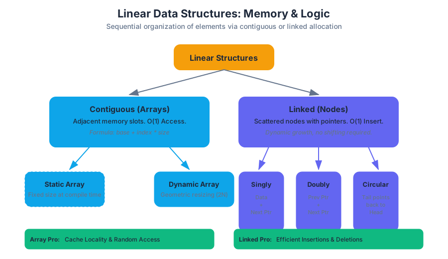
The Fundamental Dichotomy: Arrays vs. Linked Structures
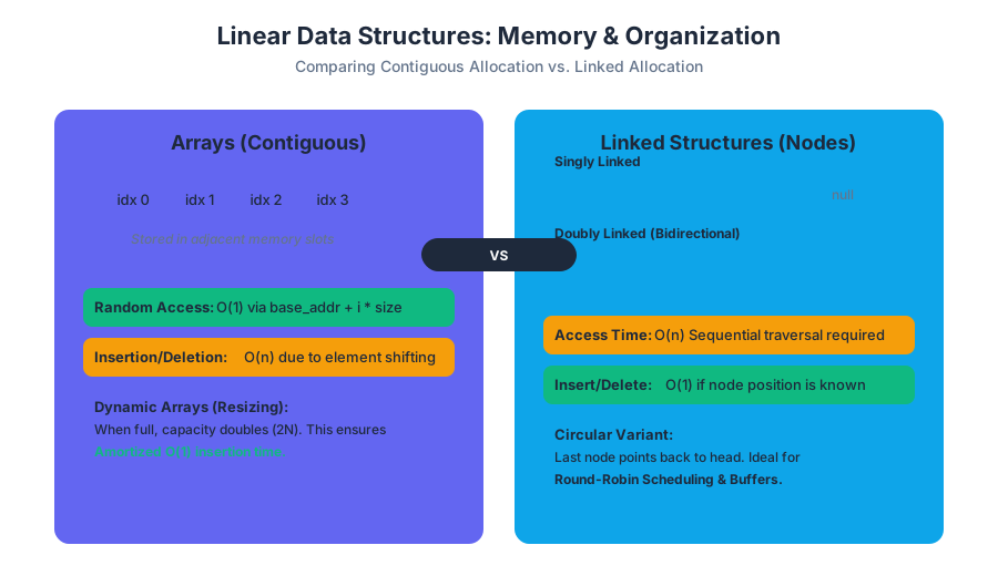
Before diving into specific types, we must understand the two primary ways linear data is stored in memory: Contiguous Allocation (Arrays) and Linked Allocation (Nodes).
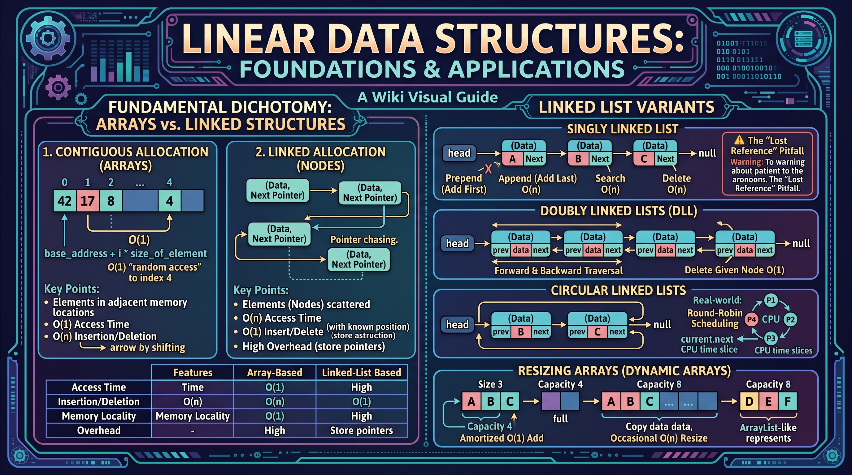
- Arrays: Elements are stored in adjacent memory locations. This allows for $O(1)$ "random access" because the address of the $i$-th element can be calculated via a simple formula:
base_address + i * size_of_element. - Linked Structures: Elements (Nodes) are scattered throughout memory. Each node contains the data and a "pointer" or "reference" to the next node. This sacrifices random access for $O(1)$ insertions and deletions at specific points.
| Feature | Array-Based | Linked-List Based |
|---|---|---|
| Access Time | $O(1)$ (Random Access) | $O(n)$ (Sequential Access) |
| Insertion/Deletion | $O(n)$ (due to shifting) | $O(1)$ (if position is known) |
| Memory Locality | Excellent (Cache friendly) | Poor (Pointer chasing) |
| Overhead | Minimal (Fixed size) | High (Store pointers for every element) |
Singly Linked Lists
A Singly Linked List is a collection of nodes where each node points to the next, ending in a null reference. It is the most basic form of a linked structure.
What it is
Mathematically, a Singly Linked List is a directed graph where every node has an out-degree of at most 1. Each node consists of a Data Field (the value) and a Next Field (the reference).
How it works
To manage a list, we typically maintain a reference to the head (the first node). If the list is empty, head is null.
public class Node {
    int data;
    Node next;

    public Node(int data) {
        this.data = data;
        this.next = null;
    }
}
Operations and Complexity
- Prepend (Add First): $O(1)$. Create a new node, point its
nextto the currenthead, and updatehead. - Append (Add Last): $O(n)$ if only
headis known; $O(1)$ if atailpointer is maintained. - Search: $O(n)$. You must traverse from the head until the value is found.
- Delete: $O(n)$ for a general value because you must find the node before the one you want to delete to update its
nextpointer.
The "Lost Reference" Pitfall: A common error in Singly Linked Lists is losing the reference to the rest of the list during an insertion or deletion. Always update the
nextpointer of the new node before breaking the link of the previous node.
Doubly Linked Lists
A Doubly Linked List (DLL) extends the singly linked list by adding a prev pointer to each node, allowing for bidirectional traversal.
Why it matters
While a DLL uses more memory (an extra pointer per node), it solves a critical weakness of the singly linked list: the inability to look backward. In a singly linked list, deleting a node requires a reference to its predecessor. In a DLL, a node "knows" its predecessor, making deletion $O(1)$ if you already have a reference to the node being deleted.
Implementation
public class DoubleNode {
    int data;
    DoubleNode next;
    DoubleNode prev;
}
Comparison of Linked List Variants
| Operation | Singly Linked | Doubly Linked | Circular (Singly) |
|---|---|---|---|
| Traverse Forward | Yes | Yes | Yes |
| Traverse Backward | No | Yes | No (unless full loop) |
| Memory per Node | $Data + 1$ Ptr | $Data + 2$ Ptrs | $Data + 1$ Ptr |
| Delete Given Node | $O(n)$ | $O(1)$ | $O(n)$ |
Circular Linked Lists
In a Circular Linked List, the last node’s next pointer does not point to null; instead, it points back to the head (or some other node in the list).
Mechanics
Circular lists are often implemented with a single tail pointer rather than a head. Why? Because tail.next is effectively the head. This gives you $O(1)$ access to both the start and the end of the list with only one pointer.
Real-World Case: Round-Robin Scheduling
Operating systems use circular lists to manage CPU time slices. Each process is a node. The CPU services the process at the current pointer, then moves to current.next. When it reaches the "end," it naturally loops back to the first process without needing a conditional reset.
Resizing Arrays (Dynamic Arrays)
Standard arrays have a fixed size. To create a "growable" list (like Java's ArrayList or Python's list), we use Resizing Arrays.
The Geometric Resizing Strategy
When the array is full and a new element is added:
- Allocate a new array of a larger size (usually $2 \times$ the current capacity).
- Copy all elements from the old array to the new one.
- Update the reference to the new array.
Why $2N$ and not $N+1$?
If we increase the size by 1 each time, adding $N$ elements takes $1 + 2 + 3 + ... + N$ operations, which is $O(N^2)$. This is catastrophically slow. By doubling the size, we ensure that the "expensive" resize happens infrequently.
Amortized Analysis
Theorem: The amortized time complexity of an insertion in a resizing array (doubling strategy) is $O(1)$.
Proof (Aggregate Method): Consider $N$ insertions into an array starting at size 1.
- The total number of copies due to resizing is $1 + 2 + 4 + 8 + ... + N/2$.
- This is a geometric series that sums to approximately $N-1$.
- Total work = $N$ (for the insertions) + $N-1$ (for the copies) $\approx 2N$.
- Average work per insertion = $2N / N = 2$, which is $O(1)$.
Common Pitfall: Thrashing
If you resize up when the array is full and resize down immediately when it is 49% full, a sequence of alternating add and remove operations at the threshold could cause $O(N)$ resizing every single time. To prevent this, we typically wait until the array is 1/4 full before shrinking it to 1/2 size.
Stacks (LIFO)
A Stack is a restricted linear data structure that follows the Last-In-First-Out (LIFO) principle. Think of a stack of physical plates: you can only add to the top and take from the top.
Key Operations
push(item): Add an item to the top.pop(): Remove and return the top item.peek(): Return the top item without removing it.
Implementation Strategies
- Linked List:
pushisaddFirst(),popisremoveFirst(). Both are $O(1)$ guaranteed. - Resizing Array:
pushadds to the end of the array. $O(1)$ amortized.
Application: Dijkstra’s Two-Stack Algorithm
Stacks are essential for parsing mathematical expressions. Consider ( 1 + ( ( 2 + 3 ) * ( 4 * 5 ) ) ).
- Value Stack: Stores operands (1, 2, 3...).
- Operator Stack: Stores operators (+, *).
- When a right parenthesis
)is encountered, pop an operator and two values, apply the operator, and push the result back onto the value stack.
Queues (FIFO)
A Queue follows the First-In-First-Out (FIFO) principle. It models a line at a grocery store: the first person to join the line is the first to be served.
Key Operations
enqueue(item): Add an item to the back (tail).dequeue(): Remove and return the item from the front (head).
The Circular Buffer (Array Implementation)
Implementing a queue with an array is trickier than a stack. If we simply remove the element at index 0, we must shift all other elements left, making dequeue $O(n)$.
To achieve $O(1)$, we use a Circular Buffer:
- Maintain
headandtailindices. - When
tailreaches the end of the array, it wraps around to index 0. - The queue is full when
(tail + 1) % capacity == head.
| Feature | Stack (LIFO) | Queue (FIFO) |
|---|---|---|
| Top/Front Operation | pop() |
dequeue() |
| Bottom/Back Operation | push() |
enqueue() |
| Primary Use Case | Backtracking, Recursion | Buffering, Scheduling |
| Search/Access | Not allowed (theoretically) | Not allowed (theoretically) |
Summary of Complexity
Understanding the performance characteristics is vital for choosing the right structure for a specific algorithm.
| Data Structure | Access | Search | Insertion (at end) | Deletion (at end) |
|---|---|---|---|---|
| Array (Fixed) | $O(1)$ | $O(n)$ | $N/A$ | $N/A$ |
| Resizing Array | $O(1)$ | $O(n)$ | $O(1)$ amortized | $O(1)$ amortized |
| Singly Linked List | $O(n)$ | $O(n)$ | $O(1)$ (w/ tail) | $O(n)$ |
| Doubly Linked List | $O(n)$ | $O(n)$ | $O(1)$ | $O(1)$ |
Advanced Pitfalls and Considerations
1. Memory Overhead
In high-performance computing, the memory overhead of linked lists is a significant deterrent. On a 64-bit system, every Node in a singly linked list carries an 8-byte pointer. If you are storing 4-byte integers, you are using 12 bytes of memory per 4 bytes of data—a 200% overhead. Arrays have near-zero overhead.
2. Cache Locality
Modern CPUs use a hierarchy of caches (L1, L2, L3). When the CPU accesses a memory address, it loads a "cache line" (usually 64 bytes) into the fast cache.
- Arrays benefit from this: accessing
arr[0]likely loadsarr[1]througharr[15]into the cache. - Linked Lists suffer from "pointer chasing": each node could be anywhere in memory, forcing the CPU to wait for a slow RAM fetch for every single element.
3. Loitering (Java/Managed Languages)
In a resizing array implementation of a stack, when you pop an element, you simply decrement the index.
public Object pop() {
    return array[--N]; // The reference array[N] still exists!
}
The reference to the object remains in the array, preventing the Garbage Collector from reclaiming that memory. This is called loitering. To fix this, you must explicitly null out the reference:
public Object pop() {
    Object item = array[--N];
    array[N] = null; // Prevent loitering
    return item;
}
Searching and Binary Search Trees
Key concepts: Binary Search · Binary Search Trees (BST) · Tree Traversal · In-order/Pre-order/Post-order
Exploration of efficient searching techniques and the hierarchical structure of Binary Search Trees.
Searching and Binary Search Trees
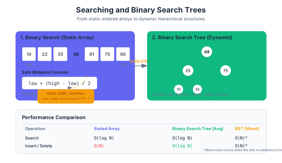
The fundamental challenge of computer science is not merely the storage of data, but its efficient retrieval. As datasets scale from thousands to billions of records, the difference between a linear search and a logarithmic search becomes the difference between a functional application and a system failure. This article explores the transition from static ordered searching to the dynamic, hierarchical world of Binary Search Trees (BSTs).
The Foundation: Binary Search on Arrays
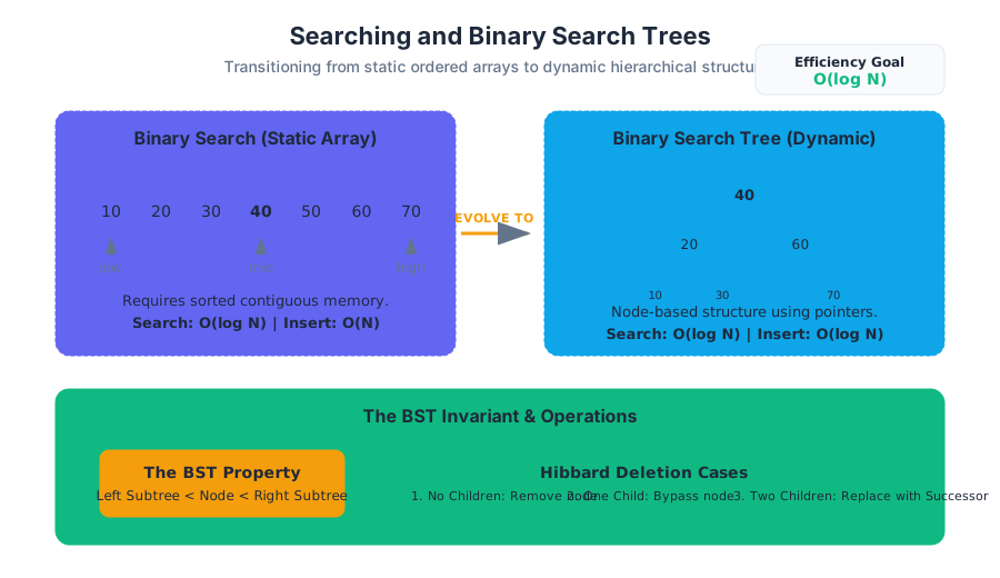
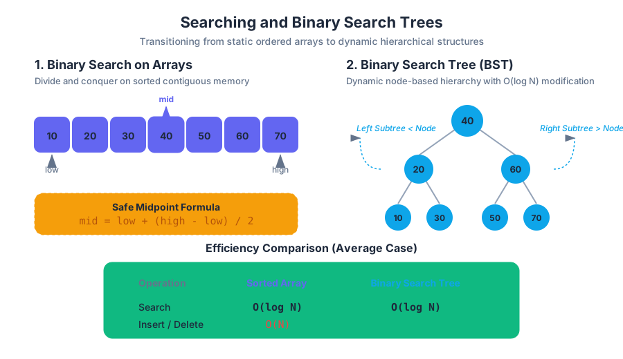
Before we can understand the complexity of tree structures, we must master the algorithm that inspired them: Binary Search. Binary search is the quintessential "divide and conquer" algorithm. It operates on the principle that if data is sorted, we can eliminate half of the search space with a single comparison.
Definition: Binary Search An algorithm that finds the position of a target value within a sorted array. It compares the target value to the middle element of the array; if they are not equal, the half in which the target cannot lie is eliminated, and the search continues on the remaining half until the target is found or the search space is empty.
The Mechanics of Binary Search
To implement binary search correctly, one must maintain two pointers, low and high, representing the current bounds of the search.
- Calculate the midpoint:
mid = low + (high - low) / 2. - Compare
array[mid]with thetarget. - If
array[mid] == target, returnmid. - If
target < array[mid], sethigh = mid - 1. - If
target > array[mid], setlow = mid + 1.
Mathematical Analysis
The efficiency of binary search is derived from the fact that the search area is halved at each step. If we have $N$ elements, after $k$ steps, we have $N/2^k$ elements remaining. The search terminates when $N/2^k = 1$, which implies $k = \log_2 N$.
| Metric | Complexity | Description |
|---|---|---|
| Best Case | $O(1)$ | The middle element is the target. |
| Average Case | $O(\log N)$ | Standard logarithmic performance. |
| Worst Case | $O(\log N)$ | Target is at the ends or not present. |
| Space Complexity | $O(1)$ | Iterative implementation uses constant space. |
Common Pitfall: The Midpoint Overflow
A classic bug in binary search is calculating the midpoint as (low + high) / 2. In many programming languages, if low + high exceeds the maximum value of a signed 32-bit integer, it will overflow to a negative number, causing an index out of bounds error. The robust way to write this is low + (high - low) / 2.
Binary Search Trees (BST)
While binary search is exceptionally fast, it requires the data to be stored in a sorted array. Arrays are "static" structures—inserting or deleting an element requires $O(N)$ time because subsequent elements must be shifted. To achieve $O(\log N)$ for both searching and modification, we move to a dynamic, node-based structure: the Binary Search Tree.
The BST Invariant
A Binary Search Tree is a binary tree where each node follows a specific ordering property:
The BST Property For any given node $X$:
- Every node in the left subtree of $X$ has a key strictly less than $X$'s key.
- Every node in the right subtree of $X$ has a key strictly greater than $X$'s key.
BST Implementation in Java
A typical BST node contains a key, an associated value, and references to its children.
public class BST<Key extends Comparable<Key>, Value> {
    private Node root;

    private class Node {
        private Key key;
        private Value val;
        private Node left, right;
        private int size; // Number of nodes in subtree

        public Node(Key key, Value val, int size) {
            this.key = key;
            this.val = val;
            this.size = size;
        }
    }

    public Value get(Key key) {
        return get(root, key);
    }

    private Value get(Node x, Key key) {
        if (x == null) return null;
        int cmp = key.compareTo(x.key);
        if      (cmp < 0) return get(x.left, key);
        else if (cmp > 0) return get(x.right, key);
        else              return x.val;
    }

    public void put(Key key, Value val) {
        root = put(root, key, val);
    }

    private Node put(Node x, Key key, Value val) {
        if (x == null) return new Node(key, val, 1);
        int cmp = key.compareTo(x.key);
        if      (cmp < 0) x.left  = put(x.left,  key, val);
        else if (cmp > 0) x.right = put(x.right, key, val);
        else              x.val   = val;
        x.size = 1 + size(x.left) + size(x.right);
        return x;
    }
}
BST Operations: Search, Insertion, and Deletion
Search and Insertion
Searching and inserting in a BST follow the same logic as binary search. We compare the target key to the current node and move left or right accordingly. Insertion always happens at a null link (a leaf position), maintaining the tree's structure.
The Challenge of Deletion (Hibbard Deletion)
Deleting a node is significantly more complex because we must maintain the BST invariant after the node is removed. There are three cases:
- Node has no children (Leaf): Simply remove the node.
- Node has one child: Replace the node with its child (bypass the node).
- Node has two children: This is the most difficult case. We must find a replacement node that is larger than everything in the left subtree and smaller than everything in the right subtree. This node is the In-order Successor (the smallest node in the right subtree).
Steps for Case 3:
- Find the node to delete ($t$).
- Find the successor ($x$) of $t$ (the minimum node in $t.right$).
- Delete the minimum from $t.right$ (using a specialized
deleteMinoperation). - Set $x.right$ to the result of the
deleteMinoperation. - Set $x.left$ to $t.left$.
- Replace $t$ with $x$.
| Operation | Average Case | Worst Case (Degenerate) |
|---|---|---|
| Search | $O(\log N)$ | $O(N)$ |
| Insert | $O(\log N)$ | $O(N)$ |
| Delete | $O(\sqrt{N})$* | $O(N)$ |
*Note: Hibbard deletion is known to slightly degrade tree balance over many operations, leading to a $\sqrt{N}$ height in some theoretical models, though $O(\log N)$ is often cited for random insertions.
Tree Traversals
Traversing a tree means visiting every node exactly once. Because trees are non-linear, there are multiple ways to define the "order" of visitation.
Depth-First Search (DFS)
DFS traversals use recursion (or a stack) to go as deep as possible before backtracking.
- In-order (Left, Root, Right): Visits nodes in ascending order. This is the most common traversal for BSTs.
- Pre-order (Root, Left, Right): Useful for creating a copy of the tree or evaluating prefix expressions.
- Post-order (Left, Right, Root): Useful for deleting the tree or evaluating postfix (Reverse Polish) expressions.
Breadth-First Search (BFS)
Also known as Level-order Traversal, this visits nodes level by level, from top to bottom and left to right. This requires a Queue data structure.
| Traversal Type | Order | Primary Use Case |
|---|---|---|
| In-order | L $\to$ Root $\to$ R | Retrieving sorted data from a BST. |
| Pre-order | Root $\to$ L $\to$ R | Serializing a tree structure. |
| Post-order | L $\to$ R $\to$ Root | Postfix math; calculating subtree sizes. |
| Level-order | Level by Level | Finding the shortest path in unweighted graphs. |
Performance Analysis and the "Degenerate" Tree
The power of the BST relies entirely on its height. In a perfectly balanced tree with $N$ nodes, the height is $\sim \log_2 N$. However, the shape of a BST depends entirely on the order of insertion.
The Worst Case: Sequential Insertion
If keys are inserted in sorted order (e.g., 1, 2, 3, 4, 5), the BST becomes a "degenerate" tree—essentially a linked list. In this state, the height $H = N$, and all operations revert to $O(N)$ time complexity.
The Average Case: Random Insertion
If keys are inserted in a random order, the height of the tree is approximately $2 \ln N$ (about $1.39 \log_2 N$). This is the mathematical justification for why BSTs are efficient in practice for most dynamic datasets.
Theorem: BST Height If $N$ distinct keys are inserted into a BST in random order, the expected number of compares for a search hit is $\sim 2 \ln N$.
Comparison of Search Structures
To understand where BSTs fit, we compare them against other fundamental searching methods:
| Structure | Search (Worst) | Insert (Worst) | Ordered Ops? |
|---|---|---|---|
| Sequential Search (Linked List) | $O(N)$ | $O(1)$ | No |
| Binary Search (Sorted Array) | $O(\log N)$ | $O(N)$ | Yes |
| BST (Basic) | $O(N)$ | $O(N)$ | Yes |
| Balanced BST (Red-Black/AVL) | $O(\log N)$ | $O(\log N)$ | Yes |
| Hash Table | $O(1)$* | $O(1)$* | No |
*Amortized average case.
Advanced Context: Balanced Search Trees and Beyond
As noted, the $O(N)$ worst-case for a basic BST is a significant liability for production systems. This led to the development of Balanced Search Trees, such as AVL Trees and Left-Leaning Red-Black Trees (LLRB).
The Core Idea of Balancing
Balanced trees use "rotations" during insertion and deletion to ensure that the height of the tree remains logarithmic regardless of the input order.
- 2-3 Trees: A theoretical construct where nodes can hold one or two keys and have two or three children. They are perfectly balanced.
- Red-Black Trees: A BST representation of a 2-3 tree. They use a "color" bit (Red or Black) on links to represent the 3-nodes of a 2-3 tree.
Connection to Sorting
There is a deep connection between BSTs and QuickSort.
- In QuickSort, the "pivot" acts like the root of a BST.
- The partitioning process in QuickSort is essentially building a BST and then performing an in-order traversal.
- The average-case complexity of both is $O(N \log N)$ for sorting and $O(\log N)$ for searching because they share the same underlying mathematical distribution.
Common Pitfalls and Best Practices
- Ignoring the Invariant: When manually modifying a tree (in an exam or a low-level implementation), always double-check that every node in the left subtree is smaller than the parent. A single misplaced node breaks the $O(\log N)$ search guarantee.
- Recursive Stack Overflow: For very deep, unbalanced trees, recursive
get()orput()calls can lead to aStackOverflowError. In production environments with potentially skewed data, iterative implementations or balanced trees are preferred. - Successor vs. Predecessor: In Hibbard deletion, you can use either the in-order successor (smallest in right subtree) or the in-order predecessor (largest in left subtree). Both are valid, but you must be consistent to avoid structural bias.
- Null Checks: Always handle the
nullcase in recursive methods. The base case for almost every BST algorithm isif (node == null).
Balanced Search Trees
Key concepts: Tree Balance · AVL Trees · Red-Black Trees · Rotations
Advanced tree structures designed to maintain logarithmic height and guarantee performance.
Balanced Search Trees
Overview
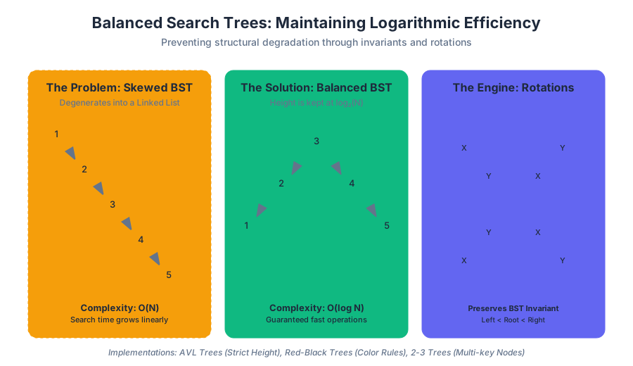
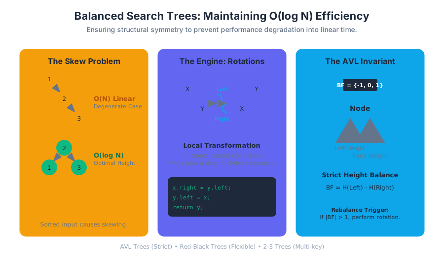
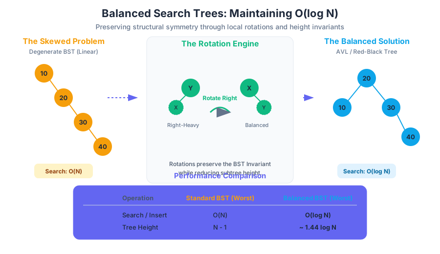
In the realm of computer science, the Binary Search Tree (BST) is a fundamental data structure designed to facilitate fast searching, insertion, and deletion. However, the efficiency of a BST is inextricably linked to its shape. A standard BST offers no guarantees regarding its structural symmetry; if keys are inserted in a sorted or semi-sorted order, the tree "skews," collapsing into a structure functionally identical to a linked list. This transformation degrades the time complexity of core operations from $O(\log N)$ to $O(N)$.
Balanced Search Trees solve this structural fragility by enforcing strict invariants. Through the use of local transformations called rotations and specific coloring or height-tracking rules, these trees ensure that the height $h$ remains logarithmic relative to the number of nodes $N$. This section explores the mechanics of balance, focusing on the two most prominent implementations: AVL Trees and Red-Black Trees.
The Balance Problem: From Logarithmic to Linear
The primary motivation for balancing a tree is the preservation of the Logarithmic Guarantee. In a perfectly balanced binary tree, the path from the root to any leaf is approximately $\log_2 N$.
The Height Theorem: For any binary tree with $N$ nodes and height $h$:
- The minimum height is $\lfloor \log_2 N \rfloor$.
- The maximum height is $N-1$ (a degenerate tree).
- The search time is proportional to the height: $O(h)$.
If we insert the keys [1, 2, 3, 4, 5] into a standard BST, we obtain a "right-leaning" chain. Every search for the value 5 requires five comparisons. In a balanced version, the same keys would result in a tree of height 2, requiring at most three comparisons.
Performance Comparison: BST vs. Balanced BST
| Operation | Average BST | Worst-case BST (Skewed) | Balanced BST (Worst-case) |
|---|---|---|---|
| Search | $O(\log N)$ | $O(N)$ | $O(\log N)$ |
| Insert | $O(\log N)$ | $O(N)$ | $O(\log N)$ |
| Delete | $O(\log N)$ | $O(N)$ | $O(\log N)$ |
| Space | $O(N)$ | $O(N)$ | $O(N)$ |
Tree Rotations: The Engine of Balance
To maintain balance without violating the BST Invariant (where for any node $x$, all keys in the left subtree are smaller than $x$ and all keys in the right subtree are larger), we use Rotations. A rotation is a local algebraic transformation that changes the parent-child relationship of a small group of nodes while preserving their relative in-order sequence.
Left Rotation (Rotate Left)
When a node $x$ has a right child $y$ that is "too heavy," we rotate $x$ to the left. $y$ becomes the new root of this subtree, and $x$ becomes the left child of $y$. If $y$ had a left child $T2$, it is reassigned as the right child of $x$.
Right Rotation (Rotate Right)
The inverse of the left rotation. If a node $y$ has a left child $x$ that is "too heavy," we rotate $y$ to the right. $x$ becomes the new root, and $y$ becomes the right child of $x$.
Rotation Implementation (Java)
private Node rotateRight(Node h) {
    // h is the node that is unbalanced to the left
    Node x = h.left;
    h.left = x.right;
    x.right = h;
    // Update metadata (height or color) here
    return x; // x is the new root of this subtree
}

private Node rotateLeft(Node h) {
    // h is the node that is unbalanced to the right
    Node x = h.right;
    h.right = x.left;
    x.left = h;
    // Update metadata (height or color) here
    return x; // x is the new root of this subtree
}
AVL Trees: Strict Height Balancing
Named after inventors Adelson-Velsky and Landis, the AVL tree was the first dynamically balanced data structure. It maintains balance by tracking the Balance Factor of every node.
The AVL Invariant: For every node in the tree, the height of the left and right subtrees can differ by at most one. $$\text{Balance Factor } (BF) = \text{height}(\text{left_subtree}) - \text{height}(\text{right_subtree})$$ A node is "balanced" if $BF \in {-1, 0, 1}$.
Rebalancing the AVL Tree
When an insertion or deletion causes a node's $BF$ to become $2$ or $-2$, a rebalancing operation is triggered. There are four distinct cases based on where the imbalance originated:
| Case | Condition | Rotation Required |
|---|---|---|
| Left-Left (LL) | New node in left-child's left-subtree | Single Right Rotation |
| Right-Right (RR) | New node in right-child's right-subtree | Single Left Rotation |
| Left-Right (LR) | New node in left-child's right-subtree | Double Rotation (Left then Right) |
| Right-Left (RL) | New node in right-child's left-subtree | Double Rotation (Right then Left) |
Worked Example: AVL Insertion
- Insert 30, 20, 10:
- 30 is root.
- 20 is left child of 30.
- 10 is left child of 20.
- Node 30 now has $BF = 2$. This is a Left-Left case.
- Action: Rotate 30 to the right. 20 becomes the root, 10 and 30 are its children. Height is now 1.
- Insert 25:
- 25 is the left child of 30.
- Tree is still balanced.
- Insert 28:
- 28 is the right child of 25.
- Node 30 now has $BF = 2$ (left height 2, right height 0). The path to the imbalance is Left (25) then Right (28). This is a Left-Right case.
- Action: Rotate 25 left, then rotate 30 right.
2-3 Search Trees: The Theoretical Ideal
Before diving into Red-Black trees, one must understand the 2-3 Tree. Unlike a binary tree, a 2-3 tree allows a node to hold more than one key.
- 2-node: One key, two children (standard BST node).
- 3-node: Two keys, three children.
- Perfect Balance Property: Every path from the root to a null link is exactly the same length.
How 2-3 Trees Grow
Instead of adding a new leaf at the bottom (which would increase height), a 2-3 tree inserts the new key into an existing leaf, temporarily creating a 4-node (3 keys, 4 children). This 4-node then "splits," sending its middle key up to the parent. If the parent becomes a 4-node, it splits again. This process ensures the tree only grows "upward" from the root, maintaining perfect balance.
Red-Black Trees: The Practical Standard
While 2-3 trees are theoretically elegant, they are difficult to implement because of the multiple node types. Red-Black Trees (specifically Left-Leaning Red-Black Trees or LLRBs) are a way to represent 2-3 trees using only standard binary nodes.
The Red-Black Mapping:
- A 2-node in a 2-3 tree is a standard black node in an RB tree.
- A 3-node in a 2-3 tree is represented as two binary nodes connected by a red link. By convention, the red link leans to the left.
Red-Black Properties
To be a valid Red-Black Tree, the following rules must hold:
- Every node is either Red or Black.
- The root is always Black.
- New insertions always start as Red.
- No two Red nodes can be adjacent (no Red child of a Red parent).
- Black Balance: Every path from the root to a null link must contain the same number of Black nodes.
Red-Black Operations
When inserting into an LLRB, we maintain balance using three primary tools:
- Rotate Left: Used to fix a right-leaning red link.
- Rotate Right: Used to fix two consecutive red links.
- Color Flip: Used to split a "4-node" (where both children are red).
private Node put(Node h, Key key, Value val) {
    if (h == null) return new Node(key, val, RED);

    int cmp = key.compareTo(h.key);
    if      (cmp < 0) h.left  = put(h.left,  key, val);
    else if (cmp > 0) h.right = put(h.right, key, val);
    else              h.val   = val;

    // 1. Right-leaning red link? Rotate left.
    if (isRed(h.right) && !isRed(h.left))      h = rotateLeft(h);
    // 2. Two red links in a row? Rotate right.
    if (isRed(h.left)  && isRed(h.left.left)) h = rotateRight(h);
    // 3. Both children red? Flip colors.
    if (isRed(h.left)  && isRed(h.right))     flipColors(h);

    return h;
}
AVL vs. Red-Black: Which to Choose?
Both structures provide $O(\log N)$ performance, but they are optimized for different workloads.
| Feature | AVL Tree | Red-Black Tree |
|---|---|---|
| Balance Strictness | Very Strict ($h < 1.44 \log N$) | Loose ($h < 2 \log N$) |
| Search Speed | Faster (due to flatter structure) | Slightly Slower |
| Insertion/Deletion | Slower (more rotations to maintain strictness) | Faster (fewer rotations) |
| Memory Overhead | Stores height (int) per node | Stores color (1 bit) per node |
| Common Use Case | Read-heavy lookups (Databases) | General purpose (Java TreeMap, C++ std::map) |
Common Pitfalls and Edge Cases
1. Forgetting the Root Color
In Red-Black trees, after any operation, the root must be explicitly set to Black. A red root doesn't necessarily break the structure, but it violates the formal definition and can lead to logic errors in complex deletions.
2. The "Double Rotation" Trap
In AVL trees, beginners often try to fix an LR (Left-Right) imbalance with a single rotation. This is impossible. A single rotation will simply move the imbalance to a different node. You must rotate the child first to convert the case into an LL (Left-Left) case, then rotate the parent.
3. Complexity of Deletion
While insertion in balanced trees is relatively straightforward, deletion is significantly more complex. In Red-Black trees, deletion often involves "Double Black" nodes and up to six different transformation cases. Most production-grade libraries use the "Bottom-Up" insertion but often implement deletion using specific "Top-Down" 2-3-4 tree logic to simplify the code.
4. Precision in Height Calculation
In AVL implementations, failing to update the height of a node after its children have been rotated is a common source of infinite loops or silent balance degradation. The height update must happen from the bottom up as the recursion unwinds.
Key Insight: The beauty of Balanced Search Trees lies in their ability to turn the "luck of the draw" (the order of input data) into a mathematical certainty. By spending a small, constant amount of time $(O(1))$ on rotations during an update, we protect the system against the catastrophic $O(N)$ failure mode.
Sorting Methodologies
Key concepts: Elementary Sorts (Selection, Insertion) · Merge Sort · Quick Sort · Heap Sort · Stability and In-place Sorting
A deep dive into various sorting algorithms, from elementary methods to efficient divide-and-conquer strategies.
Sorting Methodologies
Sorting is perhaps the most fundamental problem in computational theory. At its surface, it is the process of rearranging a sequence of objects in a specific order (typically numerical or lexicographical). However, beneath this simple definition lies a vast landscape of algorithmic strategies, memory management trade-offs, and mathematical proofs. In a production environment, the "best" sorting algorithm is rarely a single choice but rather a decision based on data distribution, hardware constraints, and stability requirements.
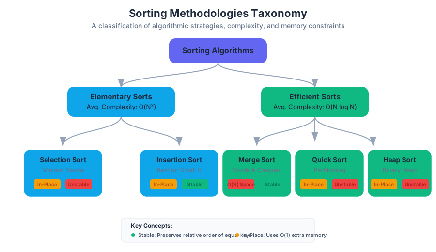
Core Definitions and Taxonomy
Before dissecting specific methodologies, we must establish the metrics by which we judge a sorting algorithm. We do not merely look at "speed"; we look at how that speed scales and how the algorithm interacts with the system's memory.
Definition: Stability A sorting algorithm is stable if it preserves the relative order of records with equal keys. If two items $A$ and $B$ have the same key and $A$ appears before $B$ in the original list, a stable sort guarantees $A$ will still appear before $B$ in the sorted list. This is critical when sorting by multiple criteria (e.g., sorting by "First Name" and then "Last Name").
Definition: In-place Sorting An algorithm is in-place if it requires only a constant amount $O(1)$ of extra memory space beyond the original array. This is vital in embedded systems or when handling massive datasets that barely fit into RAM.
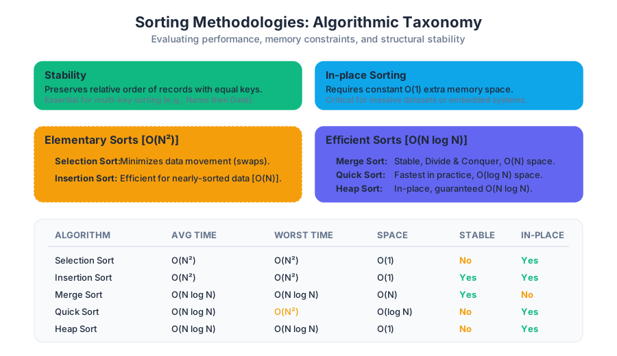
Summary of Algorithmic Characteristics
| Algorithm | Best Case | Average Case | Worst Case | Space Complexity | Stable? | In-place? |
|---|---|---|---|---|---|---|
| Selection Sort | $O(N^2)$ | $O(N^2)$ | $O(N^2)$ | $O(1)$ | No | Yes |
| Insertion Sort | $O(N)$ | $O(N^2)$ | $O(N^2)$ | $O(1)$ | Yes | Yes |
| Merge Sort | $O(N \log N)$ | $O(N \log N)$ | $O(N \log N)$ | $O(N)$ | Yes | No |
| Quick Sort | $O(N \log N)$ | $O(N \log N)$ | $O(N^2)$ | $O(\log N)$ | No | Yes |
| Heap Sort | $O(N \log N)$ | $O(N \log N)$ | $O(N \log N)$ | $O(1)$ | No | Yes |
Elementary Sorts
Elementary sorts are characterized by their $O(N^2)$ average-case complexity. While they are inefficient for large $N$, they possess small constant factors and are often used as sub-routines in more complex algorithms.
Selection Sort
Selection Sort is the most intuitive sorting method. It works by dividing the input into a "sorted" sub-list and an "unsorted" sub-list. It repeatedly finds the minimum element from the unsorted sub-list and swaps it with the leftmost unsorted element.
Mechanics:
- Maintain a pointer $i$ starting at 0.
- Scan the array from $i$ to $N-1$ to find the index
minof the smallest element. - Swap
a[i]anda[min]. - Increment $i$ and repeat until the array is exhausted.
Mathematical Analysis: The number of compares in Selection Sort is independent of the initial order of the data. For an array of size $N$, it always performs: $$(N-1) + (N-2) + \dots + 1 + 0 = \frac{N(N-1)}{2} \approx \frac{N^2}{2} \text{ compares.}$$ It performs exactly $N$ swaps. This makes Selection Sort useful when the cost of moving items is very high relative to the cost of comparing them.
Insertion Sort
Insertion Sort functions similarly to how one might sort a hand of playing cards. It processes elements one by one, inserting each into its proper place among the elements already processed.
Mechanics:
- Start with the second element (index 1).
- Compare it with the element to its left. If it is smaller, "slide" the larger elements to the right until the correct hole is found.
- Insert the element.
The Inversion Metric: Insertion Sort's performance is tied to the number of inversions in the array. An inversion is a pair of keys $(a[i], a[j])$ such that $i < j$ but $a[i] > a[j]$.
- If an array is nearly sorted (the number of inversions is $O(N)$), Insertion Sort runs in $O(N)$ time.
- This makes it the algorithm of choice for small arrays ($N < 15$) or for cleaning up data that is already mostly in order.
public class ElementarySorts {
    public static void selectionSort(Comparable[] a) {
        int N = a.length;
        for (int i = 0; i < N; i++) {
            int min = i;
            for (int j = i + 1; j < N; j++) {
                if (less(a[j], a[min])) min = j;
            }
            exch(a, i, min);
        }
    }

    public static void insertionSort(Comparable[] a) {
        int N = a.length;
        for (int i = 1; i < N; i++) {
            for (int j = i; j > 0 && less(a[j], a[j-1]); j--) {
                exch(a, j, j-1);
            }
        }
    }

    private static boolean less(Comparable v, Comparable w) {
        return v.compareTo(w) < 0;
    }

    private static void exch(Object[] a, int i, int j) {
        Object tmp = a[i];
        a[i] = a[j];
        a[j] = tmp;
    }
}
Merge Sort: The Divide and Conquer Paradigm
Merge Sort is a recursive algorithm that achieves the theoretical lower bound for comparison-based sorting: $O(N \log N)$. It is based on the principle that merging two sorted arrays is much easier than sorting a single unsorted one.
Mechanics of the Merge
The heart of the algorithm is the merge operation. Given two sorted halves of an array, we use an auxiliary array to reconstruct the full sorted sequence. We maintain three pointers: one for the left half, one for the right half, and one for the destination in the auxiliary array.
Top-Down vs. Bottom-Up
- Top-Down Merge Sort: This is the standard recursive implementation. It divides the array into halves, calls itself on those halves, and then merges.
- Bottom-Up Merge Sort: This is a non-recursive version. It starts by merging adjacent pairs of elements (size 1), then merges the resulting sorted blocks of size 2, then 4, and so on. This is often preferred in environments where recursion depth is a concern.
Mathematical Proof of Complexity: Let $T(N)$ be the number of compares to sort $N$ elements. The recurrence relation is: $$T(N) = 2T(N/2) + N$$ Using the Master Theorem, where $a=2, b=2, f(n)=n$: Since $n^{\log_b a} = n^{\log_2 2} = n^1$, and $f(n) = \Theta(n)$, we fall into Case 2. Therefore, $T(N) = \Theta(N \log N)$.
Common Pitfalls:
- Memory Overhead: Unlike the elementary sorts, Merge Sort is not in-place. It requires an auxiliary array of size $N$. In memory-constrained environments, this can be a deal-breaker.
- Recursive Depth: For very large $N$, the stack depth could theoretically lead to a
StackOverflowError, though this is rare given the $\log N$ growth.
Quick Sort: The Partitioning Paradigm
Quick Sort is widely considered the most efficient general-purpose sorting algorithm. While it has a worst-case complexity of $O(N^2)$, its average-case performance is $O(1.39 N \log N)$ with very small constant factors.
The Partitioning Step
Quick Sort works by choosing a pivot element and rearranging the array so that:
- The pivot is in its final sorted position.
- All elements to the left of the pivot are less than or equal to it.
- All elements to the right of the pivot are greater than or equal to it.
Mechanics (Hoare Partitioning):
- Pick
a[lo]as the pivot. - Scan
ifrom left to right as long asa[i] < pivot. - Scan
jfrom right to left as long asa[j] > pivot. - Swap
a[i]anda[j]. - Repeat until
iandjcross. - Swap the pivot with
a[j].
The Importance of Randomization
Quick Sort's worst case occurs when the pivot is consistently the smallest or largest element (e.g., sorting an already sorted array). To prevent this, we must shuffle the array before sorting. This guarantees that the $O(N^2)$ case is mathematically improbable (less likely than the computer being struck by a meteor).
Variations: 3-Way Partitioning (Dijkstra's Solution)
When an array contains many duplicate keys, standard Quick Sort still performs $O(N \log N)$ or even $O(N^2)$ work. 3-way partitioning (the Dutch National Flag problem) divides the array into three sections: elements less than the pivot, elements equal to the pivot, and elements greater than the pivot.
public class QuickSort {
    public static void sort(Comparable[] a) {
        StdRandom.shuffle(a); // Crucial for performance guarantee
        sort(a, 0, a.length - 1);
    }

    private static void sort(Comparable[] a, int lo, int hi) {
        if (hi <= lo) return;
        int j = partition(a, lo, hi);
        sort(a, lo, j - 1);
        sort(a, j + 1, hi);
    }

    private static int partition(Comparable[] a, int lo, int hi) {
        int i = lo, j = hi + 1;
        Comparable v = a[lo];
        while (true) {
            while (less(a[++i], v)) if (i == hi) break;
            while (less(v, a[--j])) if (j == lo) break;
            if (i >= j) break;
            exch(a, i, j);
        }
        exch(a, lo, j);
        return j;
    }
}
Heap Sort: Priority Queue Sorting
Heap Sort utilizes a Binary Heap data structure to manage elements. It is essentially a "Selection Sort" but using a sophisticated data structure to find the maximum element in $O(\log N)$ time rather than $O(N)$.
The Two Phases
- Heap Construction: We transform the raw array into a max-heap. This is done in $O(N)$ time using the "bottom-up" heapify method (sinking elements from the middle of the array to the start).
- Sortdown: We repeatedly remove the maximum element (the root of the heap), swap it with the last element of the unsorted portion, and "sink" the new root to restore the heap property.
Advantages:
- Guaranteed $O(N \log N)$: Unlike Quick Sort, there is no "worst-case" $N^2$.
- In-place: Unlike Merge Sort, it uses $O(1)$ extra space.
Disadvantages:
- Cache Locality: Heap Sort jumps around in memory (from index $i$ to $2i$ and $2i+1$). This leads to many cache misses, making it slower in practice than Quick Sort or Merge Sort on modern hardware.
- Not Stable: The swapping process destroys the relative order of equal keys.
| Strategy | Pivot/Structure | Key Advantage | Key Disadvantage |
|---|---|---|---|
| Standard Quick | First element (after shuffle) | Fastest average time | Worst case $O(N^2)$ |
| 3-Way Quick | Pivot with equal-key handling | Efficient for duplicates | Slightly more complex code |
| Heap Sort | Max-Heap structure | Guaranteed $O(N \log N)$ | Poor cache performance |
Stability and In-place Sorting: The Engineering Trade-off
In professional software engineering, the choice of sorting algorithm is often dictated by the nature of the data and the system architecture.
When to use what?
- Java
Arrays.sort(): Uses a variation of TimSort (a hybrid of Merge Sort and Insertion Sort) for Object arrays because stability is usually expected for objects. It uses Dual-Pivot Quick Sort for primitives because stability isn't required and speed is paramount. - Embedded Systems: Heap Sort is often preferred because it provides a hard guarantee on $O(N \log N)$ time and $O(1)$ space, ensuring the system never runs out of memory or hangs on a "bad" dataset.
- Large Scale Data Processing: Merge Sort is the basis for external sorting (sorting data that doesn't fit in RAM) because it accesses data sequentially, which is ideal for disk I/O or tape drives.
Comparison of Stability and Space
| Algorithm | Stable? | In-place? | Notes |
|---|---|---|---|
| Selection | No | Yes | Minimizes swaps. |
| Insertion | Yes | Yes | Best for nearly sorted data. |
| Merge | Yes | No | Guaranteed $N \log N$, high memory. |
| Quick | No | Yes | Fastest in practice, cache-friendly. |
| Heap | No | Yes | Guaranteed $N \log N$, cache-hostile. |
Common Pitfalls and Edge Cases
- The "Sorted Array" Trap: Applying Quick Sort to an already sorted array without shuffling or using a median-of-three pivot selection results in $O(N^2)$ performance.
- Duplicate Keys: Standard Quick Sort can become $O(N^2)$ if all keys are equal. 3-way partitioning is the standard fix.
- Stability Misconception: Many believe that any algorithm can be made stable easily. While true (by adding the original index to the key), it increases space complexity to $O(N)$.
- Comparator Violations: In languages like Java or C++, if your
compareToorcomparefunction does not obey the transitive property (if $a < b$ and $b < c$, then $a < c$), sorting algorithms can enter infinite loops or throw exceptions.
Theorem: The Sorting Lower Bound Any comparison-based sorting algorithm must make at least $\log_2(N!) \approx N \log_2 N$ comparisons in the worst case. This is proven via the decision tree model, where each comparison halves the number of possible permutations.
- Stability: The property of preserving the relative order of equal keys.
- In-place: An algorithm that requires $O(1)$ auxiliary memory.
- Inversion: A pair of elements in a sequence that are out of their natural order.
- Pivot: An element used in Quick Sort to partition the array into two sub-arrays.
- Heapify: The process of creating a heap data structure from a binary tree represented by an array.
- Divide and Conquer: An algorithmic paradigm that breaks a problem into smaller sub-problems, solves them, and combines the results.
- External Sorting: Sorting techniques used when the data being sorted does not fit into the main memory.
- Why is Insertion Sort preferred over Quick Sort for very small arrays?
- Explain why Merge Sort is generally preferred for sorting Linked Lists while Quick Sort is preferred for Arrays.
- If you have a dataset where every element is at most 10 positions away from its sorted position, which algorithm provides the best time complexity?
- What is the primary reason Heap Sort is rarely used in high-performance applications despite its $O(N \log N)$ guarantee?
- A system has 4GB of RAM and you need to sort a 3.5GB file. Which algorithm (Merge or Quick) is safer to use, and why?
Key Objectives:
- Understand the trade-offs between $O(N^2)$ and $O(N \log N)$ algorithms.
- Identify the role of stability in multi-key sorting.
- Master the partitioning logic of Quick Sort and the merging logic of Merge Sort.
- Recognize the impact of data distribution (duplicates, nearly sorted) on algorithmic choice.
Formula Review:
- Selection Sort Compares: $\sim N^2 / 2$
- Insertion Sort Compares (Average): $\sim N^2 / 4$
- Merge Sort Compares: $N \log_2 N$
- Quick Sort Compares (Average): $2N \ln N \approx 1.39 N \log_2 N$
Practical Implementation Tip: Always use a randomized shuffle before Quick Sort. When implementing Merge Sort, allocate the auxiliary array once and pass it through the recursive calls to avoid the overhead of repeated $O(N)$ allocations.
Directed Graphs and Shortest Paths
Key concepts: Directed Graphs (Digraphs) · Adjacency Lists · Dijkstra's Algorithm · Edge Relaxation
Modeling complex relationships using graphs and finding the most efficient paths between nodes.
Directed Graphs and Shortest Paths
The study of graphs is the study of relationships. While undirected graphs model symmetric relationships—like a physical cable connecting two routers—many real-world systems are inherently asymmetric. A one-way street, a hyperlink from one webpage to another, or a prerequisite requirement for a university course all possess a specific directionality. These are Directed Graphs, or Digraphs.
In this deep dive, we will explore the formal structure of digraphs, the efficiency of various representation methods, and the algorithmic crown jewel of graph theory: Dijkstra’s Algorithm. We will move beyond simple definitions to understand the mathematical mechanics of Edge Relaxation and the data structure optimizations that allow these algorithms to scale to the size of the modern internet.
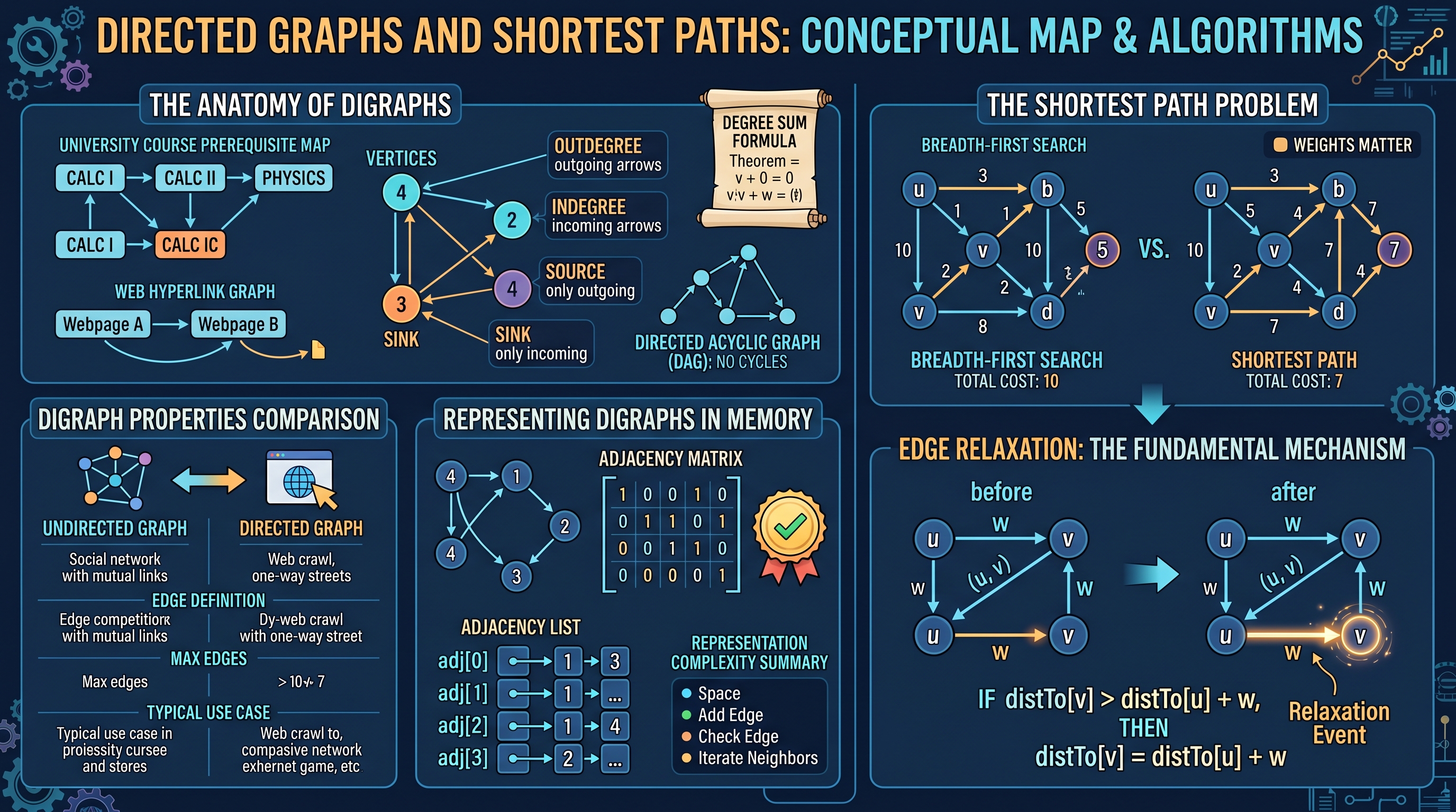
The Anatomy of Directed Graphs (Digraphs)
A Directed Graph (Digraph) is a set of vertices $V$ and a set of directed edges $E$. Each edge is an ordered pair of vertices $(u, v)$, representing a path from $u$ to $v$. Unlike undirected graphs, the existence of an edge $(u, v)$ does not imply the existence of $(v, u)$.
Formal Definitions and Terminology
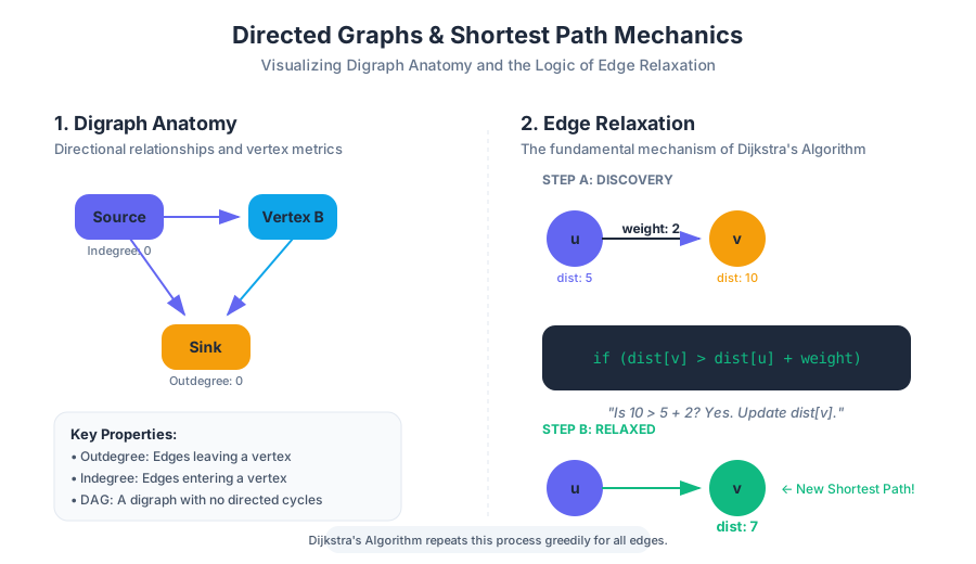
To discuss digraphs with precision, we must define the metrics of connectivity:
- Outdegree: The number of edges leaving a vertex.
- Indegree: The number of edges entering a vertex.
- Source: A vertex with an indegree of 0.
- Sink: A vertex with an outdegree of 0.
- Strong Connectivity: A digraph is strongly connected if there is a directed path between every pair of vertices.
- Directed Acyclic Graph (DAG): A digraph containing no directed cycles. These are fundamental for modeling dependencies and scheduling.
Theorem: The Degree Sum Formula for Digraphs In any digraph $G = (V, E)$, the sum of the outdegrees of all vertices is equal to the sum of the indegrees, and both are equal to the total number of edges $|E|$. $$\sum_{v \in V} outdeg(v) = \sum_{v \in V} indeg(v) = |E|$$
Digraph Properties Comparison
| Property | Undirected Graph | Directed Graph (Digraph) |
|---|---|---|
| Edge Definition | Unordered pair ${u, v}$ | Ordered pair $(u, v)$ |
| Connectivity | Connected / Disconnected | Strongly / Weakly Connected |
| Max Edges | $V(V-1)/2$ | $V(V-1)$ |
| Traversal | BFS / DFS | BFS / DFS (Direction-sensitive) |
| Typical Use Case | Social networks, Maps | Web crawls, Task scheduling |
Representing Digraphs in Memory
Choosing the right data structure is a trade-off between memory consumption and the speed of specific queries (e.g., "Is $u$ connected to $v$?").
Adjacency Matrix
An Adjacency Matrix is a 2D array of size $V \times V$. For an unweighted graph, matrix[i][j] is 1 if there is an edge from $i$ to $j$, and 0 otherwise. For weighted graphs, the cell stores the weight value.
- Pros: $O(1)$ time to check if an edge exists.
- Cons: $O(V^2)$ space complexity, which is prohibitive for sparse graphs (where $E \ll V^2$).
Adjacency List
An Adjacency List uses an array of size $V$, where each entry adj[i] points to a linked list or dynamic array of all vertices $j$ such that an edge $(i, j)$ exists.
- Pros: $O(V + E)$ space complexity. Efficient for iterating over neighbors.
- Cons: Checking if a specific edge $(u, v)$ exists takes $O(outdeg(u))$ time.
Representation Complexity Summary
| Operation | Adjacency Matrix | Adjacency List |
|---|---|---|
| Space Complexity | $O(V^2)$ | $O(V + E)$ |
| Add Edge | $O(1)$ | $O(1)$ |
| Check Edge (u, v) | $O(1)$ | $O(outdeg(u))$ |
| Iterate Neighbors of u | $O(V)$ | $O(outdeg(u))$ |
| Suitability | Dense Graphs ($E \approx V^2$) | Sparse Graphs ($E \approx V$) |
The Shortest Path Problem
In a weighted digraph, the Shortest Path from vertex $s$ to vertex $t$ is a directed path such that the sum of the weights of its constituent edges is minimized.
Why Weights Matter
In an unweighted graph, Breadth-First Search (BFS) is sufficient to find the shortest path because "shortest" simply means "fewest edges." However, in real-world scenarios—like calculating the fastest route from New York to Boston—edges have weights representing distance, time, or fuel cost. BFS fails here because a path with three short edges might be "shorter" than a path with one very long edge.
Edge Relaxation: The Fundamental Mechanism
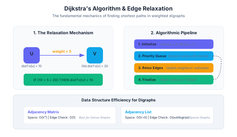
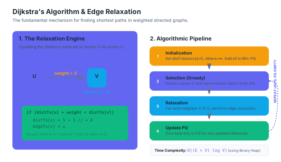
The "engine" of almost every shortest-path algorithm is Relaxation. Imagine you have an estimate of the distance from the start node $s$ to a node $v$, denoted as distTo[v]. If you discover an edge from $u$ to $v$ with weight $w$, you check if going through $u$ provides a shorter path to $v$ than your current estimate.
Definition: Relaxation For an edge $e = (u, v)$ with weight $w$: If
distTo[v] > distTo[u] + w:distTo[v] = distTo[u] + wedgeTo[v] = u
Relaxation "tightens" the distance estimate. We start with all distTo values set to infinity (except the source, which is 0) and repeatedly relax edges until we find the minimum.
Dijkstra’s Algorithm
Developed by Edsger W. Dijkstra in 1956, this algorithm is a Greedy Algorithm that solves the single-source shortest path problem for graphs with non-negative edge weights.
How It Works: The Logic
Dijkstra’s maintains a set of "visited" vertices whose shortest distance from the source is already known. In each iteration, it picks the "unvisited" vertex with the smallest current distance estimate, "visits" it, and relaxes all of its outgoing edges.
- Initialize: Set
distTo[s] = 0anddistTo[v] = ∞for all other vertices. - Priority Queue: Insert all vertices into a Min-Priority Queue (PQ) keyed by their
distTovalue. - Loop: While the PQ is not empty:
- Delete the vertex $u$ with the minimum distance from the PQ.
- For each neighbor $v$ of $u$:
- Relax the edge $(u, v)$.
- If the relaxation decreases
distTo[v], update $v$'s position in the PQ.
Implementation in Java
The following implementation uses an IndexMinPQ, a common structure in textbook implementations (like Sedgewick's) that allows for the decreaseKey operation efficiently.
public class DijkstraSP {
    private double[] distTo;          // distTo[v] = distance of shortest s->v path
    private DirectedEdge[] edgeTo;    // edgeTo[v] = last edge on shortest s->v path
    private IndexMinPQ<Double> pq;    // priority queue of vertices

    public DijkstraSP(EdgeWeightedDigraph G, int s) {
        distTo = new double[G.V()];
        edgeTo = new DirectedEdge[G.V()];

        for (int v = 0; v < G.V(); v++)
            distTo[v] = Double.POSITIVE_INFINITY;
        distTo[s] = 0.0;

        pq = new IndexMinPQ<Double>(G.V());
        pq.insert(s, 0.0);

        while (!pq.isEmpty()) {
            int v = pq.delMin();
            for (DirectedEdge e : G.adj(v))
                relax(e);
        }
    }

    private void relax(DirectedEdge e) {
        int v = e.from(), w = e.to();
        if (distTo[w] > distTo[v] + e.weight()) {
            distTo[w] = distTo[v] + e.weight();
            edgeTo[w] = e;
            if (pq.contains(w)) pq.decreaseKey(w, distTo[w]);
            else                pq.insert(w, distTo[w]);
        }
    }
}
Complexity Analysis of Dijkstra
The efficiency of Dijkstra’s algorithm depends heavily on the data structure used for the Priority Queue.
Complexity Breakdown
| PQ Implementation | insert |
delete-min |
decrease-key |
Total Time Complexity |
|---|---|---|---|---|
| Array | $O(1)$ | $O(V)$ | $O(1)$ | $O(V^2)$ |
| Binary Heap | $O(\log V)$ | $O(\log V)$ | $O(\log V)$ | $O(E \log V)$ |
| Fibonacci Heap | $O(1)$ | $O(\log V)$ | $O(1)$ (amortized) | $O(E + V \log V)$ |
For most practical applications, the Binary Heap (specifically an Indexed Binary Heap) provides the best balance of performance and implementation simplicity. In a sparse graph where $E$ is close to $V$, $E \log V$ is very efficient. In a dense graph where $E \approx V^2$, the simple array implementation $O(V^2)$ can actually be faster due to lower constant factors.
Variations and Extensions
While Dijkstra is the standard, it is not always the best tool for every job.
1. A* Search Algorithm
A* is an extension of Dijkstra used in AI and games. It uses a heuristic $h(v)$ to estimate the distance from $v$ to the goal. The priority queue is keyed by $f(v) = distTo[v] + h(v)$. If the heuristic is "admissible" (never overestimates), A* will find the shortest path much faster by "steering" the search toward the destination.
2. Directed Acyclic Graphs (DAGs)
If a graph is a DAG, we can find the shortest path in $O(V + E)$ time by relaxing vertices in Topological Order. This is even faster than Dijkstra because it doesn't require a priority queue. This method also works for finding the Longest Path in a DAG, which is useful for critical path analysis in project management.
3. Bellman-Ford Algorithm
Dijkstra fails if there are negative edge weights. If a graph has negative weights but no negative cycles, the Bellman-Ford algorithm can find the shortest path in $O(VE)$ time.
Shortest Path Algorithm Comparison
| Algorithm | Restriction | Complexity | Note |
|---|---|---|---|
| BFS | Unweighted edges | $O(V + E)$ | Only for uniform weights |
| Dijkstra | Non-negative weights | $O(E \log V)$ | Standard for most maps |
| DAG Shortest Path | No cycles | $O(V + E)$ | Uses Topological Sort |
| Bellman-Ford | No negative cycles | $O(VE)$ | Handles negative weights |
Common Pitfalls and Edge Cases
The Negative Weight Trap
A common misconception is that you can "fix" negative weights by adding a large constant to every edge weight to make them all positive. This does not work. Adding a constant $C$ to every edge penalizes paths with more edges more heavily than paths with fewer edges, potentially changing which path is the shortest.
Cycles and Infinite Loops
In a graph with a negative cycle (a cycle where the sum of weights is less than zero), a "shortest path" does not exist because you could traverse the cycle infinitely many times to achieve a distance of $-\infty$. Dijkstra’s algorithm will not detect this; it will simply produce an incorrect result. Bellman-Ford is required to detect negative cycles.
Floating Point Precision
When weights are floating-point numbers (doubles), cumulative rounding errors can occur. In high-stakes financial or scientific applications, it is often better to use integers (e.g., representing dollars as cents) to maintain precision.
Performance in Dense Graphs
In a complete graph where $E = V(V-1)$, Dijkstra’s $O(E \log V)$ becomes $O(V^2 \log V)$. In this specific case, using a simple array for the priority queue—which results in $O(V^2)$—is mathematically and practically superior.
Summary of the Shortest Path Pipeline
To solve a shortest path problem in a production environment, an engineer typically follows this pipeline:
- Identify the Graph Type: Is it directed? Are there cycles?
- Validate Weights: Are there negative weights? If yes, use Bellman-Ford. If no, proceed.
- Check for DAG structure: If it's a DAG, use Topological Sort for $O(V+E)$ performance.
- Select Data Structure: For general graphs, use Dijkstra with an Indexed Binary Heap.
- Relaxation: Iterate through the graph, relaxing edges and updating the Priority Queue until the sink is reached or the PQ is empty.
- Path Reconstruction: Use the
edgeTo[]array to backtrack from the destination to the source to retrieve the actual path.
Final Exam and Course Review
Key concepts: Exam Logistics · Regrade Policies · Comprehensive Review
Comprehensive review of course materials and logistics for the final examination.
Final Exam and Course Review
The final assessment in a data structures and algorithms course (CS112) represents the synthesis of a semester's worth of computational theory, implementation patterns, and performance analysis. This review serves as a comprehensive technical guide, bridging the gap between abstract algorithmic concepts and the rigorous demands of a final examination. Success on the final requires more than rote memorization; it demands a deep understanding of how data structures interact with memory, how algorithms scale with input size, and the trade-offs inherent in every design decision.
Administrative Logistics and Exam Protocol
The final exam is a high-stakes environment where administrative precision is as important as technical proficiency. Unlike midterms, the final is comprehensive and often follows a stricter protocol regarding identification and submission.
Exam Day Procedures
The exam typically spans a three-hour window (e.g., 4:00 PM – 7:00 PM). Students are expected to arrive at least 30 minutes early to facilitate seating and ID verification.
| Requirement | Description | Rationale |
|---|---|---|
| Valid ID | University-issued photo ID or government ID. | Mandatory for identity verification during exam submission. |
| Room Assignment | Often different from midterm locations; check the course portal. | Capacity management and proctoring optimization. |
| Materials | Usually restricted to pens/pencils; check if a "cheat sheet" is allowed. | Focus on internalizing concepts rather than external retrieval. |
Post-Exam: Grading and Regrades
Once the final is graded, results are released via platforms like Gradescope. The "Regrade Window" is notoriously narrow—often closing within 24 hours of grade release.
Regrade Policy Insight: Regrade requests are intended to correct grading errors where the rubric was applied incorrectly. They are not a platform for negotiating partial credit. Students are generally limited to one request per sub-question.
Core Concept I: Union-Find (Disjoint Sets)
The Union-Find data structure solves the Dynamic Connectivity problem. It maintains a set of elements partitioned into non-overlapping subsets.
Mechanics and Implementation
We track components using an array id[]. The two primary operations are:
find(p): Return the identifier for the component containingp.union(p, q): Merge the components containingpandq.
While the "Quick-Find" and "Quick-Union" approaches provide baseline implementations, the Weighted Quick-Union with Path Compression (WQUPC) is the gold standard for performance.
| Algorithm | Union | Find | Connected |
|---|---|---|---|
| Quick-Find | $O(N)$ | $O(1)$ | $O(1)$ |
| Quick-Union | $O(\text{tree height})$ | $O(\text{tree height})$ | $O(\text{tree height})$ |
| Weighted QU | $O(\log N)$ | $O(\log N)$ | $O(\log N)$ |
| WQUPC | $\alpha(N)^*$ | $\alpha(N)^*$ | $\alpha(N)^*$ |
| *$\alpha(N)$ is the inverse Ackermann function, which is effectively constant ($< 5$) for all practical values of $N$. |
Worked Example: Weighted Quick-Union
Suppose we have 10 elements (0-9). We perform union(4, 3), union(3, 8), and union(6, 5).
- In Weighted QU, we always attach the smaller tree to the root of the larger tree to keep the structure flat.
- If we then
union(9, 4), and 4 is the root of a tree of size 3, 9 becomes a child of 4.
public int find(int i) {
    while (i != parent[i]) {
        parent[i] = parent[parent[i]]; // Path compression (halving)
        i = parent[i];
    }
    return i;
}

public void union(int p, int q) {
    int rootP = find(p);
    int rootQ = find(q);
    if (rootP == rootQ) return;
    if (size[rootP] < size[rootQ]) {
        parent[rootP] = rootQ;
        size[rootQ] += size[rootP];
    } else {
        parent[rootQ] = rootP;
        size[rootP] += size[rootQ];
    }
}
Core Concept II: Asymptotic Analysis (Big O)
Asymptotic analysis is the mathematical framework used to describe the limiting behavior of a function. In CS112, it is used to classify algorithms by how their running time or space requirements grow as the input size $N$ grows.
The Hierarchy of Growth
Understanding the relative order of growth is critical for selecting the right algorithm for a given scale.
- Constant: $O(1)$ — Array access, basic arithmetic.
- Logarithmic: $O(\log N)$ — Binary search, balanced BST operations.
- Linear: $O(N)$ — Single loop, traversing a linked list.
- Linearithmic: $O(N \log N)$ — Merge Sort, Quick Sort (average).
- Quadratic: $O(N^2)$ — Nested loops, Elementary sorts (Selection/Insertion).
- Exponential: $O(2^N)$ — Exhaustive search, recursive Fibonacci.
Common Pitfalls in Big O
- Ignoring Constants in Small N: While $O(N^2)$ is worse than $O(N \log N)$ asymptotically, for $N=10$, an $N^2$ algorithm with a small constant might be faster.
- Confusing Best, Average, and Worst Case: Big O usually refers to the Upper Bound (worst case), while Big Omega ($\Omega$) refers to the Lower Bound. Big Theta ($\Theta$) indicates a tight bound where the upper and lower bounds match.
Core Concept III: Sorting Algorithms
Sorting is the bedrock of algorithmic study. The final exam tests the ability to distinguish between Stability, In-place execution, and Complexity.
Comparison of Sorting Methodologies
| Algorithm | Best Case | Average Case | Worst Case | Space | Stable? | In-place? |
|---|---|---|---|---|---|---|
| Selection | $O(N^2)$ | $O(N^2)$ | $O(N^2)$ | $O(1)$ | No | Yes |
| Insertion | $O(N)$ | $O(N^2)$ | $O(N^2)$ | $O(1)$ | Yes | Yes |
| Merge Sort | $O(N \log N)$ | $O(N \log N)$ | $O(N \log N)$ | $O(N)$ | Yes | No |
| Quick Sort | $O(N \log N)$ | $O(N \log N)$ | $O(N^2)$ | $O(\log N)$ | No | Yes |
Merge Sort: Divide and Conquer
Merge Sort is a recursive algorithm that splits the array into halves, sorts them, and merges the results.
- The Merge Step: Requires an auxiliary array. This is why Merge Sort is not in-place.
- Performance: Guaranteed $O(N \log N)$, making it ideal for large datasets where memory is not the primary constraint.
Quick Sort: The Partitioning Strategy
Quick Sort selects a "pivot" and partitions the array such that elements less than the pivot are on the left and greater are on the right.
- Worst Case: Occurs when the pivot is the smallest or largest element (e.g., sorting an already sorted array without shuffling).
- Optimization: Randomized shuffling before sorting guarantees $O(N \log N)$ average performance.
Core Concept IV: Search Trees
Search trees facilitate efficient retrieval, insertion, and deletion. The transition from simple Binary Search Trees (BSTs) to Balanced Trees is a major exam focus.
Binary Search Trees (BST)
A BST is a tree where each node has a key, and every node's key is larger than all keys in its left subtree and smaller than all keys in its right subtree.
- Problem: In the worst case (inserting keys in sorted order), a BST becomes a linked list, degrading performance to $O(N)$.
Balanced Search Trees (LLRB)
Left-Leaning Red-Black (LLRB) Trees are a 2-3 tree representation using binary nodes. They maintain balance by ensuring no path from the root to a leaf is more than twice as long as any other.
The Red-Link Rule: Red links lean left. No node has two red links connected to it. The tree has "perfect black balance" (every path from root to null link has the same number of black links).
Tree Rotations
Rotations are the fundamental operations used to maintain balance during insertion and deletion.
- Rotate Left: Used when a red link leans right.
- Rotate Right: Used to fix temporary 4-nodes or unbalance.
- Color Flip: Used when both children are red.
private Node rotateLeft(Node h) {
    Node x = h.right;
    h.right = x.left;
    x.left = h;
    x.color = h.color;
    h.color = RED;
    return x;
}
Core Concept V: Directed Graphs (Digraphs)
Graphs represent relationships between objects. In a Directed Graph, edges have a specific orientation (from $v$ to $w$).
Key Graph Algorithms
- Depth-First Search (DFS): Explores as far as possible along each branch before backtracking. Used for cycle detection and topological sort.
- Breadth-First Search (BFS): Explores all neighbors at the current depth before moving to the next level. Used for finding the shortest path in unweighted graphs.
- Topological Sort: An ordering of vertices such that for every directed edge $uv$, vertex $u$ comes before $v$. This is only possible in Directed Acyclic Graphs (DAGs).
| Problem | Algorithm | Complexity |
|---|---|---|
| Pathfinding (Any) | DFS | $O(V + E)$ |
| Shortest Path (Unweighted) | BFS | $O(V + E)$ |
| Cycle Detection | DFS (Stack-based) | $O(V + E)$ |
| Topological Sort | DFS (Post-order Reverse) | $O(V + E)$ |
Cycle Detection and DAGs
A Directed Acyclic Graph (DAG) is a digraph with no directed cycles. In a final exam context, you are often asked to determine if a graph is a DAG or to provide a topological ordering. If a DFS finds an edge pointing to an ancestor in the recursion stack (a "back edge"), a cycle exists.
Exam Strategy: How to Approach Problem Types
The CS112 final usually consists of three distinct problem types. Mastering each requires a different mental model.
1. Trace Problems
You are given an initial state (e.g., an array or a tree) and a sequence of operations.
- Strategy: Work slowly. For Union-Find, draw the trees. For Sorting, write out the array after each pass or partition.
- Common Error: Skipping steps. In Quick Sort partitioning, missing one swap can invalidate the entire result.
2. Code Completion/Debugging
You are given a snippet of Java code with blanks or errors.
- Strategy: Identify the "Invariants." For a BST
putmethod, remember the recursive structure:node.left = put(node.left, key, val). - Focus: Pay attention to edge cases like
nullchecks and boundary conditions in loops (i < Nvsi <= N).
3. Design and Analysis
You are given a real-world scenario and must choose the best data structure.
- Example: "You need to store a million usernames and check for duplicates instantly."
- Answer: A Hash Set or a Balanced BST. If the question asks for the usernames in alphabetical order, the Balanced BST is superior because it supports
in-ordertraversal in $O(N)$.
Summary Table: Data Structure Performance
| Structure | Search (Avg) | Search (Worst) | Insert (Avg) | Notes |
|---|---|---|---|---|
| Array (Unsorted) | $O(N)$ | $O(N)$ | $O(1)$ | Fast insert, slow search. |
| Array (Sorted) | $O(\log N)$ | $O(\log N)$ | $O(N)$ | Binary search enabled. |
| Linked List | $O(N)$ | $O(N)$ | $O(1)$ | No random access. |
| BST | $O(\log N)$ | $O(N)$ | $O(\log N)$ | Depends on input order. |
| LLRB (Balanced) | $O(\log N)$ | $O(\log N)$ | $O(\log N)$ | Guaranteed performance. |
| Hash Table | $O(1)$ | $O(N)$ | $O(1)$ | No ordering properties. |
Final Review Checklist
- Union-Find: Can you perform a
unionoperation on a Weighted Quick-Union tree and show the resulting structure? - Big O: Can you simplify $3N^2 + 10N \log N + 100$ to its asymptotic class?
- Sorting: Do you know which sorts are stable? (Merge, Insertion).
- Trees: Can you perform a
Left Rotationon a specific node in a Red-Black tree? - Graphs: Can you trace a BFS and list the order in which vertices are visited?
- Logistics: Do you have your ID and know your specific exam room?
The final exam is a test of endurance and clarity. By categorizing problems into these core domains and understanding the underlying mechanics of each data structure, you can navigate the complexities of the assessment with the precision of a senior engineer. Good luck.
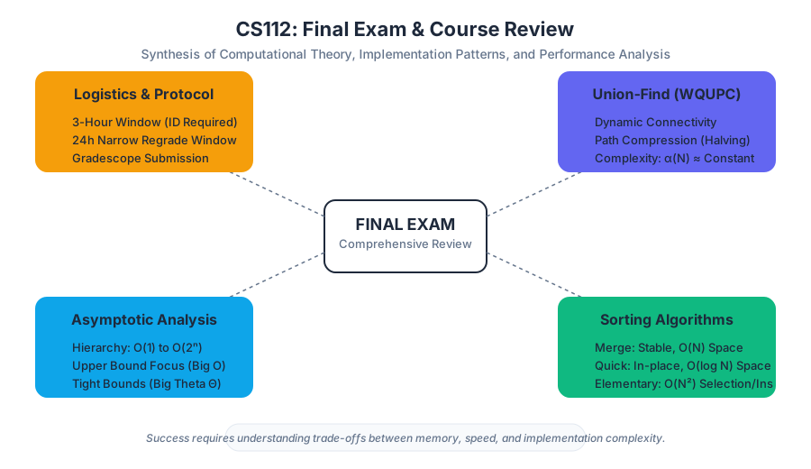
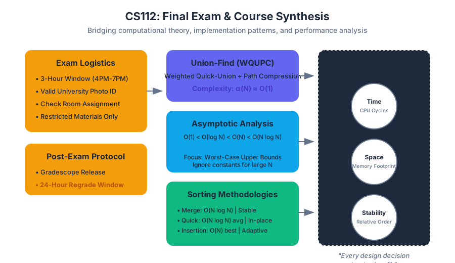
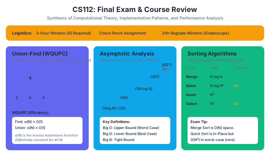
Source Materials
- Union Find and Big O Problems.mp4
- Union Find and Big O Problems.mp4
- 01B - Union Find.pdf
- 01B - Union Find.pdf
- 01B - Union Find.pdf
- 9C - Quick Sort.pdf
- Quick.java
- 02 - Stacks and Queues.pdf
- 03 - Special Linked Structures.pdf
- 02 - Stacks and Queues.pdf
- 03 - Special Linked Structures.pdf
- 02 - Stacks and Queues.pdf
Study Data Structures and Algorithmic Analysis with AI — Free on Lykke
Sign up for free to generate personalized flashcards, quizzes, and study guides from this course. Chat with an AI tutor that knows the material.
Get Started FreeView this course wiki on Lykke · Browse all public course wikis