CS323: Numerical Analysis and Computing
Institution: MIT
44 study materials · 7 sections
CS323 provides a comprehensive introduction to numerical algorithms, focusing on practical implementation and real-world applications. The course begins with the fundamentals of computational error and floating-point arithmetic before diving into core topics like solving linear systems, root-finding, and polynomial interpolation. With a heavy emphasis on programming, students will use Python, NumPy, and SciPy to implement and analyze the performance of various numerical methods. This hands-on approach prepares students to tackle computational problems in fields like machine learning, data analysis, and computer vision.
Course Sections
Foundations of Numerical Computing
Key concepts: Floating-Point Arithmetic · Absolute and Relative Error · Machine Epsilon · Catastrophic Cancellation · Big-O Notation · Python Programming Basics · Vector Norms
This section introduces the core principles of numerical analysis. It covers why numerical methods are necessary by exploring the limitations of computer arithmetic, including floating-point representation and catastrophic cancellation. Key concepts like error analysis, Big-O notation for complexity, and a practical refresher on Python programming are also provided.
Foundations of Numerical Computing
Numerical computing is the art and science of solving mathematical problems using computers. It is a discipline born from a fundamental tension: the world of mathematics is one of infinite precision and continuous values, while the world of the computer is finite and discrete. This module explores the foundational principles that govern this translation from the abstract to the practical. We begin by dissecting how computers represent numbers, a process that is inherently an approximation. This approximation introduces errors, which, if not understood and managed, can accumulate, propagate, and lead to catastrophic failures in otherwise mathematically sound algorithms. We will learn to quantify these errors, analyze their behavior, and understand the computational cost of our methods, providing the essential toolkit for any serious practitioner in science, engineering, or data analysis.
Understanding these concepts is not merely an academic exercise. An algorithm for guiding a spacecraft, simulating a climate model, or training a neural network can be perfectly correct in theory yet fail spectacularly in practice if it is not designed to handle the realities of finite-precision arithmetic. By learning to analyze error and computational complexity, you will gain the ability to distinguish between an algorithm that should work and one that will work, enabling you to design and implement solutions that are not only correct but also efficient, robust, and reliable.
Floating-Point Arithmetic
At the heart of numerical computing lies the challenge of representing the infinite set of real numbers, $\mathbb R$, using a finite number of bits. The universal standard for this task is floating-point arithmetic, a system that approximates real numbers using a binary version of scientific notation.
What It Is
A floating-point number is represented by a sign, a significand (or mantissa), and an exponent. The most common standard is IEEE 754, which defines formats like single-precision (32-bit) and double-precision (64-bit).
Definition: IEEE 754 Floating-Point Representation A number $x$ is represented as: $$ x = (-1)^S \times (1.M)_2 \times 2^{(E - \text{bias})} $$ Where:
- S is the sign bit (0 for positive, 1 for negative).
- M is the mantissa (or significand), the fractional part of the number. The leading
1.is typically implicit and not stored. - E is the exponent, an unsigned integer from which a bias is subtracted to allow for negative exponents.
The bits are allocated differently for each precision level, creating a trade-off between the range of representable numbers (governed by the exponent) and their precision (governed by the mantissa).
| Parameter | Single Precision (binary32) | Double Precision (binary64) |
|---|---|---|
| Total Bits | 32 | 64 |
| Sign Bits | 1 | 1 |
| Exponent Bits | 8 | 11 |
| Mantissa Bits | 23 (+1 implicit) | 52 (+1 implicit) |
| Exponent Bias | 127 | 1023 |
| Smallest Normal | $\approx 1.18 \times 10^{-38}$ | $\approx 2.23 \times 10^{-308}$ |
| Largest Normal | $\approx 3.40 \times 10^{38}$ | $\approx 1.80 \times 10^{308}$ |
Why It Matters
Because the mantissa and exponent have a finite number of bits, the set of representable floating-point numbers, known as machine numbers, is a finite subset of the real numbers. Any real number that does not have an exact finite binary representation must be approximated, typically by rounding to the nearest machine number. This fundamental act of approximation is the original sin of numerical computing and the source of rounding error.
How It Works: A Concrete Example
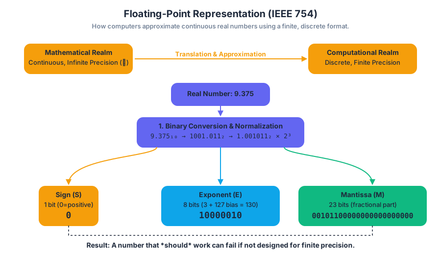
Let's represent the decimal number 9.375 in single precision.
- Sign: The number is positive, so
S = 0. - Binary Conversion:
9.375in binary is1001.011. - Normalization: In binary scientific notation, this is
1.001011 * 2^3. - Mantissa: The fractional part is
001011. We pad this to 23 bits:M = 00101100000000000000000. - Exponent: The exponent is
3. We add the bias:E = 3 + 127 = 130. In 8-bit binary, this is10000010.
Putting it together, the 32-bit representation is:
0 (Sign) 10000010 (Exponent) 00101100000000000000000 (Mantissa)
This example worked perfectly because 9.375 has an exact finite binary representation. A number like 0.1 does not, and must be rounded, introducing an immediate error.
Low-Level Implementation
To truly see the bit-level representation, we can use a low-level language like C with a union to access the same memory location as both a float and an unsigned int.
#include <stdio.h>
#include <stdint.h>

// A union allows us to interpret the same 4 bytes of memory
// in different ways without type-casting.
typedef union {
    float f;
    uint32_t u;
} FloatIntUnion;

// Function to print the bits of a 32-bit unsigned integer
void print_bits(uint32_t n) {
    for (int i = 31; i >= 0; i--) {
        printf("%d", (n >> i) & 1);
        if (i == 31 || i == 23) {
            printf(" "); // Add space for readability
        }
    }
    printf("\n");
}

int main() {
    FloatIntUnion fiu;
    fiu.f = 9.375f;

    printf("Representing: %f\n", fiu.f);
    printf("Hex representation: 0x%08X\n", fiu.u);
    printf("Binary representation (S EEEEEEEE MMM...):\n");
    print_bits(fiu.u);

    return 0;
}
Output:
Representing: 9.375000
Hex representation: 0x41160000
Binary representation (S EEEEEEEE MMM...):
0 10000010 00101100000000000000000
This output perfectly matches our manual derivation and demonstrates the concrete structure of a floating-point number in memory.
Absolute and Relative Error
Since floating-point arithmetic is an approximation, we need a formal language to describe the discrepancy between a true value and its computed approximation.
What It Is
Let $x_{true}$ be the exact value and $x_{approx}$ be its approximation.
Definition: Absolute Error The absolute error is the magnitude of the difference between the true and approximate values. $$ E_{abs} = |x_{true} - x_{approx}| $$
Definition: Relative Error The relative error is the absolute error scaled by the magnitude of the true value. $$ E_{rel} = \frac{|x_{true} - x_{approx}|}{|x_{true}|} \quad (\text{for } x_{true} \neq 0) $$
Why It Matters
Absolute error is useful, but it lacks context. An absolute error of 1 cm is excellent when measuring the distance between cities but catastrophic when manufacturing a CPU. Relative error is often the more meaningful metric because it is dimensionless and expresses the error as a fraction of the true value's magnitude. In most scientific and engineering contexts, we are concerned with controlling the relative error of our computations.
Error Propagation
A crucial aspect of error analysis is understanding how errors from initial approximations propagate through arithmetic operations. Let's analyze the subtraction of two approximate numbers, $\bar{x} \approx x$ and $\bar{y} \approx y$. Let the relative errors be $\delta_x$ and $\delta_y$, such that $\bar{x} = x(1 + \delta_x)$ and $\bar{y} = y(1 + \delta_y)$.
\begin{aligned}
\text{The computed difference is } \bar{z} &= \bar{x} - \bar{y} \\
&= x(1 + \delta_x) - y(1 + \delta_y) \\
&= (x - y) + (x\delta_x - y\delta_y)
\end{aligned}

\text{The absolute error in the result is } E_{abs} &= |\bar{z} - (x-y)| = |x\delta_x - y\delta_y|

\text{The relative error in the result is } E_{rel} &= \frac{|x\delta_x - y\delta_y|}{|x-y|}
This final expression is the key. If $x \approx y$, the denominator $|x-y|$ becomes very small. Even if $\delta_x$ and $\delta_y$ are tiny, the relative error $E_{rel}$ can become enormous. This phenomenon is a direct precursor to catastrophic cancellation.
Machine Epsilon
Machine epsilon is a fundamental constant of a given floating-point system that quantifies its maximum possible relative error due to rounding.
What It Is
Definition: Machine Epsilon ($\varepsilon_{mach}$) Machine epsilon is the difference between 1 and the next larger representable floating-point number.
It is not the smallest positive number a system can represent. Rather, it defines the resolution of the number line around the value 1.0. For any real number $x$, when it is rounded to its nearest floating-point representation fl(x), the following relationship holds:
$$ \text{fl}(x) = x(1 + \delta), \quad \text{where } |\delta| \le \varepsilon_{mach} $$
This means machine epsilon is the upper bound on the relative error incurred when representing a real number as a machine number.
| Precision | Machine Epsilon ($\varepsilon_{mach}$) | Value |
|---|---|---|
| Single (32-bit) | $2^{-23}$ | $\approx 1.19 \times 10^{-7}$ |
| Double (64-bit) | $2^{-52}$ | $\approx 2.22 \times 10^{-16}$ |
Why It Matters
Machine epsilon is the gold standard for judging the accuracy of numerical algorithms. It tells us the best we can hope for. If an algorithm produces a relative error on the order of $\varepsilon_{mach}$, it is considered numerically stable and as accurate as possible for that precision. It also provides a practical tolerance for convergence checks and floating-point comparisons. Instead of checking if a == b, one should check if abs(a - b) < tol, where tol is often a multiple of $\varepsilon_{mach}$.
Finding Machine Epsilon Empirically
We can write a simple program to determine the machine epsilon of our system. The logic is to find the smallest number eps such that 1.0 + eps is computationally distinguishable from 1.0.
import numpy as np

def find_machine_epsilon_float32():
    """Empirically computes machine epsilon for a 32-bit float."""
    # Start with a 32-bit floating point one
    eps = np.float32(1.0)

    # Repeatedly halve eps until 1.0 + eps is indistinguishable from 1.0
    while np.float32(1.0) + eps / np.float32(2.0) != np.float32(1.0):
        eps = eps / np.float32(2.0)

    return eps

def find_machine_epsilon_float64():
    """Empirically computes machine epsilon for a 64-bit float."""
    eps = 1.0
    while 1.0 + eps / 2.0 != 1.0:
        eps /= 2.0
    return eps

# --- Main execution ---
eps32_empirical = find_machine_epsilon_float32()
eps64_empirical = find_machine_epsilon_float64()

# Get the true values from NumPy for comparison
eps32_numpy = np.finfo(np.float32).eps
eps64_numpy = np.finfo(np.float64).eps

print("--- 32-bit Single Precision ---")
print(f"Empirically found epsilon: {eps32_empirical:.8e}")
print(f"NumPy's reported epsilon:  {eps32_numpy:.8e}")
print("-" * 30)
print("--- 64-bit Double Precision ---")
print(f"Empirically found epsilon: {eps64_empirical:.17e}")
print(f"NumPy's reported epsilon:  {eps64_numpy:.17e}")
Output:
--- 32-bit Single Precision ---
Empirically found epsilon: 1.19209290e-07
NumPy's reported epsilon:  1.19209290e-07
------------------------------
--- 64-bit Double Precision ---
Empirically found epsilon: 2.22044604925031308e-16
NumPy's reported epsilon:  2.22044604925031308e-16
This demonstrates that our simple algorithm correctly identifies the machine epsilon, confirming our understanding of its definition.
Catastrophic Cancellation
This is arguably the most insidious and common source of large numerical errors. It is a direct consequence of the finite precision of floating-point arithmetic combined with the subtraction operation.
What It Is
Definition: Catastrophic Cancellation A severe loss of significant digits that occurs when subtracting two nearly equal numbers. The result is a number with a much smaller magnitude, where the remaining digits are dominated by the rounding errors of the original numbers, leading to a massive increase in relative error.
How It Works
Imagine we are working with a toy floating-point system that stores only 5 significant decimal digits. Let's subtract $y = 123.45$ from $x = 123.46$.
- True result: $x - y = 0.01$.
- Now, suppose $x$ and $y$ are themselves the result of some prior calculation and have small rounding errors in their last digit. Let's say our stored values are $\bar{x} = 123.46(123...)$ and $\bar{y} = 123.45(456...)$.
- Our 5-digit system rounds them to $\bar{x}{stored} = 1.2346 \times 10^2$ and $\bar{y}{stored} = 1.2345 \times 10^2$.
- The subtraction is performed: $\bar{x}{stored} - \bar{y}{stored} = 0.0001 \times 10^2 = 0.01$.
The result seems correct. But the five significant digits we started with (1, 2, 3, 4, 6 and 1, 2, 3, 4, 5) have been reduced to just one (1). The other four digits of our result are now effectively zero. If there were any noise or error in the digits that were cancelled out, that noise now constitutes 100% of the non-zero part of our result. The relative error has been magnified enormously, just as predicted by our error propagation formula.
Concrete Example: The Quadratic Formula
A classic example is solving the quadratic equation $ax^2 + bx + c = 0$ using the standard formula: $$ x = \frac{-b \pm \sqrt{b^2 - 4ac}}{2a} $$ Consider the case where $b^2 \gg 4ac$. In this situation, $\sqrt{b^2 - 4ac} \approx |b|$. If $b > 0$, the root $x_1 = (-b + \sqrt{b^2 - 4ac}) / 2a$ involves subtracting two nearly equal numbers, leading to catastrophic cancellation.
The solution is to use a mathematically equivalent but numerically stable formulation. We can calculate the stable root first (the one that uses addition) and then use Vieta's formula, $x_1 x_2 = c/a$, to find the second root accurately.
import numpy as np

def quadratic_naive(a, b, c):
    """Solves ax^2 + bx + c = 0 using the naive formula."""
    # Use 64-bit floats for precision
    a, b, c = float(a), float(b), float(c)
    discriminant = np.sqrt(b**2 - 4*a*c)
    x1 = (-b + discriminant) / (2*a)
    x2 = (-b - discriminant) / (2*a)
    return x1, x2

def quadratic_stable(a, b, c):
    """Solves ax^2 + bx + c = 0 using a numerically stable method."""
    a, b, c = float(a), float(b), float(c)
    discriminant = np.sqrt(b**2 - 4*a*c)

    # The root with the larger magnitude is always stable because it involves addition
    # of numbers with the same sign.
    # We use np.sign(b) to handle both b > 0 and b < 0 cases.
    x1_stable = (-b - np.sign(b) * discriminant) / (2*a)

    # Use Vieta's formula to find the second root, avoiding cancellation.
    x2_stable = c / (a * x1_stable)

    # Return in conventional order
    if b > 0:
        return x2_stable, x1_stable
    else:
        return x1_stable, x2_stable

# --- Demonstration with a problematic case ---
a = 1
b = 1e8
c = 1

# The true roots are approximately -1e8 and -1e-8
print("Problem: a=1, b=1e8, c=1")
print("-" * 40)

# Naive method
x1_n, x2_n = quadratic_naive(a, b, c)
print(f"Naive method roots:    x1 = {x1_n:<25.15f}, x2 = {x2_n:<25.15f}")

# Stable method
x1_s, x2_s = quadratic_stable(a, b, c)
print(f"Stable method roots:   x1 = {x1_s:<25.15f}, x2 = {x2_s:<25.15f}")

# True value for the small root is approximately -c/b
true_x1 = -1e-8
rel_error_naive = abs(x1_n - true_x1) / abs(true_x1)
print(f"\nRelative error of small root (naive): {rel_error_naive:.2%}")
Output:
Problem: a=1, b=1e8, c=1
----------------------------------------
Naive method roots:    x1 = 0.00000000000000000, x2 = -100000000.00000000000000000
Stable method roots:   x1 = -0.000000010000000, x2 = -100000000.00000000000000000

Relative error of small root (naive): 100.00%
The naive method completely fails to find the small root, returning zero. The stable method, by reformulating the problem to avoid subtraction of nearly equal numbers, computes it with full precision.
Big-O Notation
While error analysis tells us about the accuracy of an algorithm, order notation (or Big-O notation) tells us about its efficiency. It provides a standardized way to describe an algorithm's complexity or performance as the size of its input grows.
What It Is
Definition: Big-O Notation Let $f(n)$ and $g(n)$ be two functions defined on the set of positive integers. We say that $f(n) = O(g(n))$ (read as "$f$ is big-oh of $g$") if there exist a positive constant $C$ and an integer $n_0$ such that: $$ |f(n)| \le C|g(n)| \quad \text{for all } n \ge n_0 $$
In essence, $g(n)$ provides an asymptotic upper bound for the growth of $f(n)$. We are not concerned with the exact runtime, but rather the rate of growth of the runtime. Big-O simplifies analysis by ignoring constant factors and lower-order terms. For example, if an algorithm's runtime is $T(n) = 5n^2 + 100n + 50$, we say its complexity is $O(n^2)$, because for large $n$, the $n^2$ term dominates all others.
Why It Matters
Big-O notation is the language of scalability. It allows us to compare algorithms and predict how they will perform on larger inputs. An algorithm with $O(n)$ complexity will likely outperform one with $O(n^2)$ complexity for large $n$, regardless of the specific hardware or implementation details. This is critical for designing systems that can handle real-world data sizes.
Common Complexity Classes
| Notation | Name | Example |
|---|---|---|
| $O(1)$ | Constant | Accessing an array element by index. |
| $O(\log n)$ | Logarithmic | Binary search in a sorted array. |
| $O(n)$ | Linear | Finding the maximum element in an unsorted list. |
| $O(n \log n)$ | Log-linear | Efficient sorting algorithms (e.g., Merge Sort, Quicksort). |
| $O(n^2)$ | Quadratic | Naive matrix-vector multiplication, bubble sort. |
| $O(n^3)$ | Cubic | Naive matrix-matrix multiplication. |
| $O(2^n)$ | Exponential | Traveling salesman problem (brute-force). |
| $O(n!)$ | Factorial | Permutation-based brute-force algorithms. |
Analyzing an Algorithm in Pseudocode
Let's analyze the complexity of a standard matrix-vector multiplication algorithm.
function matrix_vector_product(A, x):
  // A is an m x n matrix, x is an n-dimensional vector
  // The result y will be an m-dimensional vector

  let y be a new m-dimensional vector, initialized to zeros

  // Outer loop iterates over the rows of the matrix A
  for i from 1 to m:       // This loop runs m times

    // Inner loop iterates over the columns of A (and elements of x)
    for j from 1 to n:     // This loop runs n times

      // The core operation: a multiplication and an addition
      y[i] = y[i] + A[i,j] * x[j] // This is an O(1) operation

  return y
Analysis:
- The innermost operation (multiplication and addition) takes constant time, $O(1)$.
- The inner loop runs
ntimes. So, the total work for one iteration of the outer loop is $n \times O(1) = O(n)$. - The outer loop runs
mtimes, and each time it does $O(n)$ work. - The total complexity is therefore $m \times O(n) = O(mn)$. If the matrix is square ($m=n$), the complexity is $O(n^2)$.
Python Programming Basics for Numerical Work
While the theoretical foundations are language-agnostic, their practical implementation requires a suitable tool. For modern scientific computing, the Python ecosystem, particularly the NumPy library, is the de facto standard.
Why Python and NumPy?
- High-Level and Readable: Python's syntax is clean and expressive, allowing scientists and engineers to focus on the problem rather than on low-level memory management.
- Vast Ecosystem: Libraries like NumPy, SciPy, Matplotlib, and Pandas provide a powerful, integrated environment for computation, analysis, and visualization.
- Performance through Vectorization: Pure Python can be slow for numerical loops. NumPy provides a data structure, the
ndarray, which is a highly optimized, contiguous block of memory. Operations on these arrays are performed by pre-compiled C or Fortran code, a concept known as vectorization. This allows for performance that rivals low-level languages while retaining Python's ease of use.
A Practical Demonstration: Vectorization
Let's compare the performance of calculating the dot product of two large vectors using a pure Python loop versus a vectorized NumPy function.
# First, ensure you have numpy installed
pip install numpy
import numpy as np
import time

# Create two large random vectors
vector_size = 10_000_000
vec_a = np.random.rand(vector_size)
vec_b = np.random.rand(vector_size)
py_vec_a = list(vec_a)
py_vec_b = list(vec_b)

# --- Method 1: Pure Python loop ---
def python_dot_product(a, b):
    result = 0.0
    for i in range(len(a)):
        result += a[i] * b[i]
    return result

start_time = time.time()
py_result = python_dot_product(py_vec_a, py_vec_b)
end_time = time.time()
python_duration = end_time - start_time
print(f"Pure Python dot product took: {python_duration:.6f} seconds")

# --- Method 2: Vectorized NumPy ---
start_time = time.time()
# NumPy has multiple ways to do this: np.dot(), @ operator, or .dot() method
np_result = np.dot(vec_a, vec_b)
end_time = time.time()
numpy_duration = end_time - start_time
print(f"NumPy (vectorized) dot product took: {numpy_duration:.6f} seconds")

# --- Verification and Performance Comparison ---
print(f"\nResults are close: {np.isclose(py_result, np_result)}")
if numpy_duration > 0:
    speedup = python_duration / numpy_duration
    print(f"NumPy was approximately {speedup:.1f}x faster.")
Typical Output:
Pure Python dot product took: 1.153421 seconds
NumPy (vectorized) dot product took: 0.007982 seconds

Results are close: True
NumPy was approximately 144.5x faster.
This stark difference illustrates the power of vectorization. By offloading the loop to optimized, low-level code via NumPy, we achieve a massive performance gain. This principle is central to writing efficient numerical code in Python.
Numerical Linear Algebra: Vectors, Matrices, and Norms
Key concepts: Vector and Matrix Algebra · Vector Operations · Linear Independence · Column Space & Null Space · Vector Norms (L1, L2, L-infinity) · Matrix Norms · Condition Number
This section reviews the fundamental building blocks of numerical linear algebra. It covers the definitions and operations of vectors and matrices, key theoretical concepts like span and column space, and the crucial idea of norms for measuring the magnitude of vectors and matrices. Understanding norms is essential for analyzing error and the sensitivity of linear systems.
Numerical Linear Algebra: Vectors, Matrices, and Norms
In most real-world applications, from simulating fluid dynamics to training a deep neural network, we rarely operate on single numbers. Instead, numerical computation is performed on entire collections of numbers. Vector and matrix algebra provides the fundamental mathematical framework for organizing, manipulating, and analyzing this data. This section provides a deep dive into the essential tools of this framework: vectors, matrices, and the concept of a norm, which allows us to measure the 'size' or 'magnitude' of these objects. This ability to quantify size is the bedrock for analyzing the error, stability, and convergence of nearly all numerical algorithms.
Vectors: The Building Blocks
At its core, linear algebra is the study of vectors and the linear transformations that act upon them. Vectors are the fundamental objects, representing points in space, quantities with direction, or simply ordered lists of data.
Definition and Notation
A vector in
n-dimensional real space, denotedv ∈ ℝⁿ, is an orderedn-tuple of real numbers.v = (v₁, v₂, ..., vₙ)
By convention in numerical linear algebra, a vector is treated as a column vector, which is an n × 1 matrix:
v = \begin{pmatrix} v_1 \\ v_2 \\ \vdots \\ v_n \end{pmatrix}
Its transpose, vᵀ, is a row vector, which is a 1 × n matrix: vᵀ = $$ \begin{pmatrix} v_1 & v_2 & \dots & v_n \end{pmatrix} $$ . This distinction is not merely pedantic; it becomes critical when performing matrix operations. The space ℝⁿ is the set of all such n-dimensional vectors.
Fundamental Vector Operations
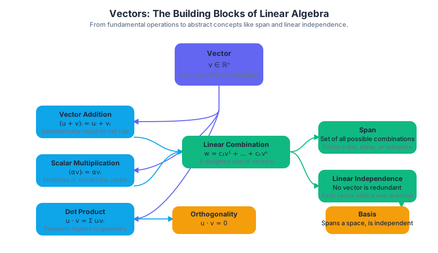
The power of vectors comes from the algebraic structure defined on ℝⁿ. The two primary operations are vector addition and scalar multiplication.
-
Vector Addition: If
u, v ∈ ℝⁿ, their sumu + vis defined by component-wise addition:(u + v)ᵢ = uᵢ + vᵢ. Geometrically, this corresponds to the "head-to-tail" rule, forming a parallelogram. -
Scalar Multiplication: If
v ∈ ℝⁿandα ∈ ℝis a scalar, their productαvis defined by multiplying each component ofvbyα:(αv)ᵢ = αvᵢ. Geometrically, this scales the vector, stretching or shrinking it and possibly reversing its direction ifα < 0.
These two operations together allow us to form linear combinations.
- Dot Product (Inner Product): The dot product of two vectors
u, v ∈ ℝⁿis a scalar value defined as:u ⋅ v = uᵀv = Σᵢ uᵢvᵢ.
The dot product is immensely useful as it connects algebra to geometry. It can be used to find the length of a vector and the angle between two vectors. The geometric definition of the dot product is u ⋅ v = ||u|| ||v|| cos(θ), where θ is the angle between u and v. This shows that two non-zero vectors are orthogonal (perpendicular) if and only if their dot product is zero.
Concrete Example: Vector Operations in Code
While high-level libraries provide optimized routines, implementing these operations from scratch reveals their underlying mechanics.
import numpy as np
import math

def manual_dot_product(v1: np.ndarray, v2: np.ndarray) -> float:
    """
    Computes the dot product of two 1D NumPy arrays without using np.dot or @.
    This demonstrates the fundamental summation algorithm.
    """
    if v1.shape != v2.shape or v1.ndim != 1:
        raise ValueError("Vectors must be 1D and have the same shape.")

    dot_product_sum = 0.0
    for i in range(v1.shape[0]):
        dot_product_sum += v1[i] * v2[i]
    return dot_product_sum

# --- Example Usage ---
u = np.array([1.0, -2.0, 3.0])
v = np.array([4.0, 5.0, 6.0])

# Scalar multiplication and vector addition
w = 2 * u + v
print(f"Vector u = {u}")
print(f"Vector v = {v}")
print(f"Result of 2*u + v = {w}\n")

# Dot product comparison
manual_result = manual_dot_product(u, v)
numpy_result = np.dot(u, v)
operator_result = u @ v # Python 3.5+ infix operator for matrix multiplication

print(f"Manual dot product: {manual_result}")
print(f"NumPy's np.dot result: {numpy_result}")
print(f"Using @ operator: {operator_result}\n")

# Geometric application: finding the angle between u and v
# cos(theta) = (u . v) / (||u|| ||v||)
norm_u = math.sqrt(manual_dot_product(u, u))
norm_v = math.sqrt(manual_dot_product(v, v))
cos_theta = manual_result / (norm_u * norm_v)
angle_rad = math.acos(cos_theta)
angle_deg = math.degrees(angle_rad)

print(f"Norm of u: {norm_u:.4f}")
print(f"Norm of v: {norm_v:.4f}")
print(f"Angle between u and v: {angle_deg:.2f} degrees")
Linear Combinations, Span, and Linear Independence
These concepts form the theoretical foundation of vector spaces.
-
A linear combination of a set of vectors
{v¹, v², ..., vᵏ}is any vectorwthat can be written asw = c₁v¹ + c₂v² + ... + cₖvᵏ, wherecᵢare scalar coefficients. -
The span of a set of vectors is the set of all possible linear combinations of those vectors. The span of a set of vectors in
ℝⁿforms a subspace ofℝⁿ(e.g., a line or a plane passing through the origin). -
A set of vectors
{v¹, v², ..., vᵏ}is linearly independent if the only solution to the equationc₁v¹ + c₂v² + ... + cₖvᵏ = 0isc₁ = c₂ = ... = cₖ = 0. Intuitively, this means no vector in the set can be expressed as a linear combination of the others. They each contribute a unique, non-redundant direction. If a set is not linearly independent, it is linearly dependent.
Why it matters: Linear independence is a cornerstone concept. In solving systems of equations, it tells us whether a solution is unique. In data science, it relates to multicollinearity, where features are redundant. A set of n linearly independent vectors in ℝⁿ forms a basis for that space, meaning any vector in ℝⁿ can be uniquely represented as a linear combination of these basis vectors.
Matrices: Linear Transformations Encapsulated
A matrix can be viewed in several ways: as a grid of numbers, a collection of vectors, or, most powerfully, as an object that represents a linear transformation between vector spaces.
Definition and Notation
An
m × nmatrixAis a rectangular array of numbers withmrows andncolumns. We writeA ∈ ℝ^(m×n). The entry in thei-th row andj-th column is denotedAᵢⱼoraᵢⱼ.
A = \begin{pmatrix}
A_{11} & A_{12} & \dots & A_{1n} \\
A_{21} & A_{22} & \dots & A_{2n} \\
\vdots & \vdots & \ddots & \vdots \\
A_{m1} & A_{m2} & \dots & A_{mn}
\end{pmatrix}
Matrix-Vector Multiplication
The product of an m × n matrix A and an n × 1 vector x results in an m × 1 vector y. This operation, y = Ax, is the engine of linear algebra and has two fundamental interpretations.
Interpretation 1: Row-wise (Dot Products) Each component
yᵢof the output vectoryis the dot product of thei-th row ofAwith the vectorx.
yᵢ = Aᵢ,₁x₁ + Aᵢ,₂x₂ + ... + Aᵢ,ₙxₙ = Σⱼ Aᵢⱼxⱼ
Interpretation 2: Column-wise (Linear Combination) The output vector
yis a linear combination of the columns ofA, where the coefficients are the components ofx.
y = x₁A₁,: + x₂A₂,: + ... + xₙAₙ,:
The column-wise view is often more insightful. It reveals that the output Ax must lie within the span of the columns of A.
// Let A be an m x n matrix and x be an n x 1 vector.
// The product y = Ax is an m x 1 vector.

// Interpretation 1: Dot products with rows
y_i = \sum_{j=1}^{n} A_{ij} x_j \quad \text{for } i=1, \ldots, m

// Example for y_1:
y_1 = (A_{1,1} * x_1) + (A_{1,2} * x_2) + \dots + (A_{1,n} * x_n)

// Interpretation 2: Linear combination of columns
// Let A_{:,j} be the j-th column of A.
y = x_1 A_{:,1} + x_2 A_{:,2} + \dots + x_n A_{:,n}

// Example:
\begin{pmatrix} y_1 \\ \vdots \\ y_m \end{pmatrix} = x_1 \begin{pmatrix} A_{1,1} \\ \vdots \\ A_{m,1} \end{pmatrix} + x_2 \begin{pmatrix} A_{1,2} \\ \vdots \\ A_{m,2} \end{pmatrix} + \dots + x_n \begin{pmatrix} A_{1,n} \\ \vdots \\ A_{m,n} \end{pmatrix}
Column Space & Null Space
These two subspaces are intrinsically linked to any matrix A ∈ ℝ^(m×n) and are critical for understanding the behavior of the linear system Ax = b.
-
Column Space
C(A): The column space ofAis the span of its column vectors. It is a subspace of the output spaceℝᵐ.- What it is: The set of all possible output vectors
bfor which the systemAx = bhas a solution. - Why it matters: If a vector
bis not inC(A), thenAx = bis inconsistent and has no solution. The dimension ofC(A)is the rank of the matrix,rank(A) = r.
- What it is: The set of all possible output vectors
-
Null Space
N(A): The null space ofAis the set of all input vectorsxthat are mapped to the zero vector. It is a subspace of the input spaceℝⁿ.- What it is: The set of all solutions to the homogeneous equation
Ax = 0. - Why it matters: The null space tells us about the uniqueness of solutions. If
N(A)contains only the zero vector, then the solution toAx = b(if it exists) is unique. IfN(A)is non-trivial, there are infinitely many solutions. The dimension ofN(A)is the nullity of the matrix.
- What it is: The set of all solutions to the homogeneous equation
These two spaces are part of the Four Fundamental Subspaces of linear algebra, which provide a complete geometric picture of a linear transformation.
| Subspace | Definition | Resides in | Dimension | Interpretation |
|---|---|---|---|---|
Column Space C(A) |
Span of columns of A |
ℝᵐ |
r (rank) |
All possible outputs b for Ax=b |
Null Space N(A) |
All x such that Ax=0 |
ℝⁿ |
n-r |
Solutions to the homogeneous equation |
Row Space C(Aᵀ) |
Span of rows of A |
ℝⁿ |
r (rank) |
Orthogonal complement of N(A) |
Left Null Space N(Aᵀ) |
All y such that Aᵀy=0 |
ℝᵐ |
m-r |
Orthogonal complement of C(A) |
This structure leads to a profound result: the Rank-Nullity Theorem.
Theorem (Rank-Nullity): For any matrix
A ∈ ℝ^(m×n), the dimension of its column space (rank) plus the dimension of its null space (nullity) equals the number of columnsn.
rank(A) + nullity(A) = n
This theorem provides a beautiful accounting of dimensions. It states that the number of dimensions in the input space (n) is split between the dimensions that are preserved and mapped to the output space (rank) and the dimensions that are collapsed to zero (nullity).
Vector Norms: Measuring Magnitude
In numerical analysis, we constantly need to quantify the size of vectors, especially error vectors. A norm is a function that generalizes the concept of "length" or "magnitude" to vector spaces.
Formal Definition of a Norm
A function ||.|| : ℝⁿ → ℝ is a vector norm if for any vectors x, y ∈ ℝⁿ and any scalar α ∈ ℝ, it satisfies:
- Non-negativity:
||x|| ≥ 0, and||x|| = 0if and only ifx = 0. - Absolute Scalability (Homogeneity):
||αx|| = |α| ||x||. - Triangle Inequality:
||x + y|| ≤ ||x|| + ||y||.
The triangle inequality is the most important property. It formalizes the idea that the shortest path between two points is a straight line.
The p-Norms: A Family of Measures
A broad and useful family of norms are the p-norms (or Lp-norms), defined as:
||x||_p = (Σᵢ |xᵢ|^p)^(1/p) for p ≥ 1.
The three most common instances of p-norms are essential tools in scientific computing and machine learning.
-
L1 Norm (
p=1, Manhattan Norm):||x||₁ = Σᵢ |xᵢ|.- How it works: It sums the absolute values of the components. It's called the "Manhattan norm" because it represents the distance a taxi would travel on a grid of streets.
- Why it matters: The L1 norm is widely used in machine learning (e.g., Lasso regression) because it promotes sparsity. Minimizing the L1 norm of a vector of parameters tends to drive many of the parameters to exactly zero, effectively performing feature selection.
-
L2 Norm (
p=2, Euclidean Norm):||x||₂ = sqrt(Σᵢ xᵢ²).- How it works: This is the standard geometric length of a vector, calculated via the Pythagorean theorem. It is the square root of the dot product of a vector with itself:
||x||₂ = sqrt(xᵀx). - Why it matters: It is the most natural measure of distance. It is used everywhere, from calculating residuals in least-squares problems to regularization in Ridge regression. Unlike the L1 norm, it is differentiable everywhere (except at the origin), which is a convenient property for optimization algorithms.
- How it works: This is the standard geometric length of a vector, calculated via the Pythagorean theorem. It is the square root of the dot product of a vector with itself:
-
L-infinity Norm (
p→∞, Max Norm):||x||_∞ = maxᵢ |xᵢ|.- How it works: It is simply the largest absolute value among the components of the vector.
- Why it matters: The L-infinity norm is used when we care about the worst-case error. It isolates the component with the maximum magnitude, which is often crucial in error analysis and ensuring stability.
Geometric Interpretation and Use Cases
The "unit ball" for each norm (the set of all vectors x such that ||x|| ≤ 1) reveals their geometric character.
| Norm | Formula | Geometric Shape (Unit Ball in ℝ²) | Common Use Case |
|---|---|---|---|
| L1 Norm (` | x | ||
| L2 Norm (` | x | ||
| L-infinity Norm (` | x |
Real-World Usage: Gradient Clipping in Deep Learning
In training deep neural networks, gradients can sometimes become excessively large, leading to unstable training. A common technique to prevent this is gradient clipping, which uses a norm to rescale gradients if their magnitude exceeds a threshold.
import torch

# Imagine this is a gradient tensor for a layer's weights during backpropagation
gradients = torch.tensor([-2.5, 0.8, 1.2, -4.0, 0.1])

# Calculate different norms of the gradient vector
l1_norm = torch.linalg.vector_norm(gradients, ord=1)
l2_norm = torch.linalg.vector_norm(gradients, ord=2)
linf_norm = torch.linalg.vector_norm(gradients, ord=float('inf'))

print(f"Gradient Tensor: {gradients}")
print(f"L1 Norm (Sum of absolute values): {l1_norm:.4f}")
print(f"L2 Norm (Euclidean length): {l2_norm:.4f}")
print(f"L-infinity Norm (Max absolute value): {linf_norm:.4f}")

# A common use case: Gradient Clipping by L2 norm
# If the L2 norm of the gradients exceeds a threshold, scale it down.
max_norm_threshold = 2.0
if l2_norm > max_norm_threshold:
    clip_coefficient = max_norm_threshold / l2_norm
    clipped_gradients = gradients * clip_coefficient

    print(f"\nL2 norm ({l2_norm:.2f}) exceeded threshold {max_norm_threshold}. Gradients clipped.")
    print(f"Clipped Gradients: {clipped_gradients}")
    print(f"New L2 Norm: {torch.linalg.vector_norm(clipped_gradients, ord=2):.4f}")
Matrix Norms: Quantifying Amplification
Just as we need to measure the size of vectors, we also need to measure the "size" or "strength" of matrices. A matrix norm quantifies the maximum effect a matrix can have on a vector.
Induced (or Operator) Norms
The most natural way to define a matrix norm is by its action on vectors. An induced norm measures the maximum "stretching factor" that the matrix applies to any vector, as measured by a specific vector norm.
The matrix norm
||A||induced by a vector norm||.||is defined as:||A|| = sup_{x≠0} (||Ax|| / ||x||) = sup_{||x||=1} ||Ax||
This definition means the matrix norm is the largest possible value of the ratio ||Ax|| / ||x||. It answers the question: "What is the maximum amplification this matrix can produce?"
Each vector p-norm induces a corresponding matrix p-norm.
- Matrix 1-Norm:
||A||₁ = max_j Σᵢ |Aᵢⱼ|(Maximum absolute column sum). - Matrix ∞-Norm:
||A||_∞ = max_i Σⱼ |Aᵢⱼ|(Maximum absolute row sum). - Matrix 2-Norm (Spectral Norm):
||A||₂ = σ_max(A), whereσ_maxis the largest singular value ofA. This norm corresponds to the true maximum stretching factor but is the most computationally expensive to calculate.
The Frobenius Norm: An Alternative View
Not all matrix norms are induced. The Frobenius norm is a commonly used alternative that is easier to compute. It treats the matrix as if it were a single long vector and calculates its L2 norm.
The Frobenius norm of a matrix
A ∈ ℝ^(m×n)is defined as:||A||_F = sqrt(Σᵢ Σⱼ Aᵢⱼ²) = sqrt(tr(AᵀA))
Pitfall: While the Frobenius norm is a valid matrix norm (it satisfies the three defining properties), it is not an induced norm. It does not represent the maximum amplification factor in the same way ||A||₂ does. However, its computational simplicity makes it popular for applications like low-rank matrix approximation.
| Norm | Type | Formula | Computational Cost |
|---|---|---|---|
| Matrix 1-Norm (` | A | ||
| Matrix ∞-Norm (` | A | ||
| Matrix 2-Norm (` | A | ||
| Frobenius Norm (` | A |
Example: Calculating Matrix Norms from the Command Line
We can use command-line tools like Octave/MATLAB for quick calculations, demonstrating another environment where these concepts are applied.
# Using octave-cli for a quick, interactive calculation of various norms for a matrix.
# This shows how these concepts are built into numerical computing environments.

# Define a 2x2 matrix A = [[1, -7], [-2, -3]]
octave-cli --eval "A = [1, -7; -2, -3]; \
                   norm_1 = norm(A, 1); \
                   norm_inf = norm(A, inf); \
                   norm_2 = norm(A, 2); \
                   norm_fro = norm(A, 'fro'); \
                   printf('Matrix A:\n'); disp(A); \
                   printf('1-Norm (max col sum of |1|+|-2|=3 and |-7|+|-3|=10): %f\n', norm_1); \
                   printf('Inf-Norm (max row sum of |1|+|-7|=8 and |-2|+|-3|=5): %f\n', norm_inf); \
                   printf('2-Norm (spectral norm, max singular value): %f\n', norm_2); \
                   printf('Frobenius Norm (sqrt(1^2 + (-7)^2 + (-2)^2 + (-3)^2)): %f\n', norm_fro);"
Output:
Matrix A:
   1  -7
  -2  -3

1-Norm (max col sum of |1|+|-2|=3 and |-7|+|-3|=10): 10.000000
Inf-Norm (max row sum of |1|+|-7|=8 and |-2|+|-3|=5): 8.000000
2-Norm (spectral norm, max singular value): 7.333245
Frobenius Norm (sqrt(1^2 + (-7)^2 + (-2)^2 + (-3)^2)): 7.937254
This example clearly shows that different norms give different measures of the "size" of the same matrix, each with its own interpretation and use case. The concepts of norms are the foundation for the condition number of a matrix, which is one of the most critical quantities in numerical analysis for determining the stability and reliability of a solution to a linear system.
Solving Systems of Linear Equations (Ax=b)
Key concepts: Direct Methods · Iterative Methods · LU Factorization · Gaussian Elimination · Pivoting Strategies · Jacobi Method · Gauss-Seidel Method · Least Squares & Normal Equations · Computational Cost
This section explores the primary methods for solving systems of linear equations, a cornerstone of numerical computing. It contrasts direct methods like LU factorization with iterative methods such as Jacobi and Gauss-Seidel, analyzing their computational costs and stability. The section also covers the practical importance of pivoting and introduces least squares for solving overdetermined systems.
Solving Systems of Linear Equations (Ax=b)
The problem of solving a system of linear equations is one of the most fundamental and ubiquitous tasks in computational science. Represented in matrix form as Ax = b, where A is a known n x n matrix of coefficients, b is a known n x 1 column vector of constants, and x is the n x 1 column vector of unknown variables, this equation appears in fields as diverse as structural engineering, circuit analysis, machine learning, and economic modeling.
At its core, solving Ax = b means finding the vector x that, when transformed by the matrix A, yields the vector b. Geometrically, it's equivalent to finding the unique linear combination of the columns of A that produces b. The methods for finding this solution fall into two broad categories: direct methods, which compute the solution in a fixed number of steps, and iterative methods, which refine an initial guess until a desired level of accuracy is reached. The choice between these approaches depends critically on the size, structure, and properties of the matrix A.
This article provides a deep dive into the theory, implementation, and practical considerations of the most important algorithms for solving Ax=b.
Direct Methods: Finite-Step Solutions
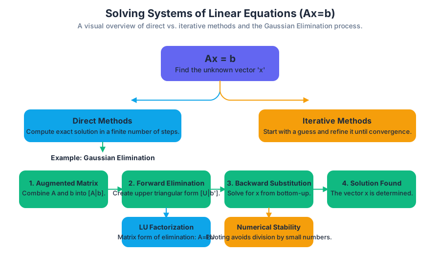
Direct methods are algorithms that find the exact solution to Ax=b in a finite and predetermined number of computational steps, assuming perfect arithmetic without any round-off errors. For a system of n equations, the number of operations is a fixed function of n. The foundational algorithm for this class of methods is Gaussian Elimination, which is more formally and efficiently implemented in modern software as LU Factorization.
Gaussian Elimination
What It Is
Gaussian Elimination is the classical algorithm for solving linear systems. It systematically transforms a system of equations into an equivalent upper triangular system, which can then be easily solved using a process called back substitution. The transformation is achieved by applying a sequence of elementary row operations:
- Swapping two rows.
- Multiplying a row by a non-zero scalar.
- Adding a multiple of one row to another row.
Key Insight: Applying these operations to the augmented matrix
[A|b]does not change the solutionxof the system. The goal is to use these operations to introduce zeros below the main diagonal of theAportion of the matrix.
How It Works
The algorithm proceeds in two main phases:
-
Forward Elimination: The goal is to convert the matrix
Ainto an upper triangular matrixU. This is done column by column.- For the first column, use the first row (the pivot row) to create zeros in all entries below the first element (
A[1,1]). This is done by subtracting a suitable multiple of the first row from each subsequent row. - For the second column, use the second row to create zeros in all entries below the second diagonal element (
A[2,2]). - This process continues for
n-1columns.
- For the first column, use the first row (the pivot row) to create zeros in all entries below the first element (
-
Backward Substitution: After forward elimination, the augmented matrix is in the form
[U|b'], whereUis upper triangular. The systemUx = b'can be solved easily, starting from the last equation.- The last equation involves only
x_n, so it can be solved directly:x_n = b'_n / U[n,n]. - The second-to-last equation involves
x_nandx_{n-1}. Sincex_nis now known,x_{n-1}can be solved for. - This process continues backward until all components of
xare found.
- The last equation involves only
Concrete Example
Consider the system:
2x₁ +  x₂ -  x₃ =  8
-3x₁ -  x₂ + 2x₃ = -11
-2x₁ +  x₂ + 2x₃ = -3
The augmented matrix is:
[ 2   1  -1 |  8 ]
[-3  -1   2 | -11]
[-2   1   2 | -3 ]
Step 1: Forward Elimination
- Target: Zeros in the first column below the diagonal.
R₂ → R₂ - (-3/2) * R₁R₃ → R₃ - (-2/2) * R₁The matrix becomes:
[ 2   1    -1   |   8  ]
[ 0  1/2   1/2  |   1  ]
[ 0   2     1   |   5  ]
- Target: Zero in the second column below the diagonal.
R₃ → R₃ - (2 / (1/2)) * R₂ = R₃ - 4 * R₂The matrix becomes:
[ 2   1    -1   |   8  ]
[ 0  1/2   1/2  |   1  ]
[ 0   0    -1   |   1  ]
The system is now upper triangular.
Step 2: Backward Substitution The new system of equations is:
2x₁ +  x₂ -  x₃ =  8
     1/2x₂ + 1/2x₃ =  1
            -x₃ =  1
- From the last equation:
x₃ = -1. - Substitute into the second equation:
1/2x₂ + 1/2(-1) = 1⇒1/2x₂ = 3/2⇒x₂ = 3. - Substitute into the first equation:
2x₁ + (3) - (-1) = 8⇒2x₁ + 4 = 8⇒2x₁ = 4⇒x₁ = 2.
The solution is x = [2, 3, -1]ᵀ.
Common Pitfalls
The naive algorithm fails if a diagonal element (a pivot) used for elimination is zero. Even worse, if a pivot is very small relative to other entries, the algorithm becomes numerically unstable due to floating-point errors. This happens because we divide by the pivot, and division by a small number amplifies any existing round-off error. This critical issue motivates the need for pivoting strategies.
LU Factorization: A Formalization of Elimination
What It Is
LU Factorization (or LU Decomposition) is the matrix representation of Gaussian Elimination. It decomposes a square matrix A into the product of a lower triangular matrix L and an upper triangular matrix U.
A = LU
Definition:
- A lower triangular matrix
Lhas all its entries above the main diagonal equal to zero (L[i,j] = 0fori < j). - An upper triangular matrix
Uhas all its entries below the main diagonal equal to zero (U[i,j] = 0fori > j).
By convention, the diagonal elements of L are set to 1 (this is called a Doolittle decomposition). The matrix U is the same upper triangular matrix obtained from Gaussian Elimination. The matrix L stores the multipliers used during the elimination process.
Why It Matters
LU factorization decouples the elimination process (which depends only on A) from the vector b. The decomposition A = LU needs to be computed only once. Then, to solve Ax=b for any given b, we solve two much simpler triangular systems:
- Substitute
A=LUintoAx=bto getLUx = b. - Define an intermediate vector
y = Ux. - First, solve
Ly = bfory. This is called forward substitution. - Then, solve
Ux = yforx. This is called backward substitution.
This is extremely efficient when solving a system with the same coefficient matrix A but many different right-hand side vectors b. The expensive O(n³) decomposition is done once, and each subsequent solve only requires two O(n²) substitutions.
How It Works
The U matrix is the result of the forward elimination phase of Gaussian Elimination. The L matrix is constructed from the multipliers used. Specifically, if we subtract m_{ij} times row j from row i to create a zero at position (i,j), then the entry L[i,j] is exactly m_{ij}.
Let's implement Doolittle's algorithm, which computes L and U directly.
import numpy as np

def lu_factorization(A):
    """
    Performs LU factorization of a square matrix A using Doolittle's algorithm.
    A = LU, where L is lower triangular with unit diagonal, and U is upper triangular.

    Args:
        A (np.ndarray): A square n x n matrix.

    Returns:
        (np.ndarray, np.ndarray): A tuple containing the L and U matrices.
    """
    n = A.shape[0]
    if A.shape[1] != n:
        raise ValueError("Input matrix must be square.")

    L = np.zeros((n, n))
    U = np.zeros((n, n))

    for k in range(n):
        # Set diagonal of L to 1
        L[k, k] = 1.0

        # Calculate U for the current row k
        # U[k, j] = A[k, j] - sum(L[k, i] * U[i, j] for i in 0..k-1)
        for j in range(k, n):
            sum_lu = sum(L[k, i] * U[i, j] for i in range(k))
            U[k, j] = A[k, j] - sum_lu

        # Calculate L for the current column k
        # L[i, k] = (A[i, k] - sum(L[i, j] * U[j, k] for j in 0..k-1)) / U[k, k]
        for i in range(k + 1, n):
            if U[k, k] == 0:
                # This indicates the matrix is singular or requires pivoting.
                # A robust implementation would handle this with pivoting.
                raise np.linalg.LinAlgError("Zero pivot encountered. Pivoting is required.")
            sum_lu = sum(L[i, j] * U[j, k] for j in range(k))
            L[i, k] = (A[i, k] - sum_lu) / U[k, k]

    return L, U

# Example from the Gaussian Elimination section
A = np.array([[2., 1., -1.],
              [-3., -1., 2.],
              [-2., 1., 2.]])

L, U = lu_factorization(A)

print("Matrix A:\n", A)
print("\nLower Triangular L:\n", L)
print("\nUpper Triangular U:\n", U)
print("\nVerification (L @ U):\n", L @ U)
Pivoting Strategies: Ensuring Numerical Stability
What It Is
As noted, Gaussian Elimination and LU Factorization can fail or become numerically unstable if a pivot element A[k,k] is zero or very small. Pivoting is a strategy of reordering the rows (and/or columns) of the matrix during factorization to ensure that the pivot element is as large as possible.
Why It Matters
Using a large pivot element minimizes the magnitude of the multipliers m_{ij}. This prevents the subtraction of nearly equal numbers and reduces the propagation of round-off errors, making the algorithm dramatically more stable and reliable in floating-point arithmetic. For all practical purposes, direct solvers are always implemented with pivoting.
How It Works
The most common strategy is Partial Pivoting:
- At step
kof the elimination (for columnk), search for the element with the largest absolute value in the current column at or below the diagonal (A[i,k]fori >= k). - Let this largest element be at row
p. - Swap row
kwith rowp. - Proceed with the elimination step as usual, using the new, larger pivot element
A[k,k].
This process of row-swapping can be represented by a permutation matrix P. A permutation matrix is an identity matrix with its rows reordered. Applying pivoting to A is equivalent to performing the factorization on a row-permuted version of A. The resulting factorization is:
PA = LU
To solve Ax=b, we first apply the same permutations to b by computing Pb, and then solve the system LUx = Pb.
Mathematical Representation of Pivoting
Without pivoting, the decomposition is A = LU. With partial pivoting, we introduce a permutation matrix P that encodes all the row swaps performed during the factorization.
// Without Pivoting:
A = \begin{pmatrix} 2 & 1 & -1 \\ -3 & -1 & 2 \\ -2 & 1 & 2 \end{pmatrix}
  = \begin{pmatrix} 1 & 0 & 0 \\ -1.5 & 1 & 0 \\ -1 & 4 & 1 \end{pmatrix}
    \begin{pmatrix} 2 & 1 & -1 \\ 0 & 0.5 & 0.5 \\ 0 & 0 & -1 \end{pmatrix}
  = L \cdot U

// With Partial Pivoting:
// At step 1, the largest element in column 1 is -3 (row 2). Swap R1 and R2.
// This corresponds to a permutation matrix P1.
P_1 = \begin{pmatrix} 0 & 1 & 0 \\ 1 & 0 & 0 \\ 0 & 0 & 1 \end{pmatrix}
A' = P_1 A = \begin{pmatrix} -3 & -1 & 2 \\ 2 & 1 & -1 \\ -2 & 1 & 2 \end{pmatrix}

// Now we factor A'. The process continues, potentially with more swaps.
// The final result is PA = LU, where P is the product of all permutation matrices.
// For our example, the final P would be:
P = \begin{pmatrix} 0 & 1 & 0 \\ 0 & 0 & 1 \\ 1 & 0 & 0 \end{pmatrix}

// The factorization becomes PA = LU, which is numerically stable.
Iterative Methods: Refining an Initial Guess
For very large and sparse systems (where most entries in A are zero), direct methods like LU factorization become computationally prohibitive. The O(n³) complexity is too high, and a more subtle problem called fill-in occurs: the L and U factors of a sparse matrix can be much denser than the original matrix A, leading to excessive memory usage.
Iterative methods provide an alternative. They start with an initial guess for the solution, x^(0), and iteratively generate a sequence of approximations x^(1), x^(2), ... that (ideally) converge to the true solution.
General Form: Most simple iterative methods can be expressed as a fixed-point iteration:
x^(k+1) = T * x^(k) + cwhereTis the iteration matrix andcis a vector, both derived fromAandb. The method converges if and only if the spectral radius (the largest absolute eigenvalue) ofTis less than 1.
A sufficient (but not necessary) condition for convergence of many methods is that the matrix A is strictly diagonally dominant.
Definition: Strictly Diagonally Dominant A matrix
Ais strictly diagonally dominant if, for every row, the absolute value of the diagonal element is greater than the sum of the absolute values of all other elements in that row.|A[i,i]| > Σ_{j≠i} |A[i,j]|for alli.
The Jacobi Method
What It Is
The Jacobi method is the simplest iterative scheme. To compute the i-th component of the new approximation x_i^(k+1), it uses only the components from the previous approximation x^(k). All components of the new vector are computed simultaneously (or in parallel) before updating.
How It Works (Derivation)
- Decompose the matrix
Ainto its diagonal (D), strictly lower triangular (-L*), and strictly upper triangular (-U*) parts:A = D - L* - U*. - The system
Ax=bbecomes(D - L* - U*)x = b. - Isolate the term with the diagonal matrix:
Dx = (L* + U*)x + b. - This naturally suggests an iterative formula by using the old
xon the right to compute the newxon the left:Dx^(k+1) = (L* + U*)x^(k) + b - Solving for
x^(k+1)gives the Jacobi iteration:x^(k+1) = D⁻¹(L* + U*)x^(k) + D⁻¹b
In component form, the update rule for each x_i is:
x_i^(k+1) = (1 / A[i,i]) * (b_i - Σ_{j≠i} A[i,j] * x_j^(k))
Concrete Example
Consider the diagonally dominant system:
4x₁ -  x₂ -  x₃ = 1
-x₁ + 4x₂ -  x₃ = 4
-x₁ -  x₂ + 4x₃ = -7
Let the initial guess be x^(0) = [0, 0, 0]ᵀ.
Iteration 1:
x₁^(1) = (1/4) * (1 - (-1*0) - (-1*0)) = 0.25
x₂^(1) = (1/4) * (4 - (-1*0) - (-1*0)) = 1.0
x₃^(1) = (1/4) * (-7 - (-1*0) - (-1*0)) = -1.75
So, x^(1) = [0.25, 1.0, -1.75]ᵀ.
Iteration 2:
x₁^(2) = (1/4) * (1 - (-1*1.0) - (-1*-1.75)) = (1/4) * (1 + 1.0 - 1.75) = 0.0625
x₂^(2) = (1/4) * (4 - (-1*0.25) - (-1*-1.75)) = (1/4) * (4 + 0.25 - 1.75) = 0.625
x₃^(2) = (1/4) * (-7 - (-1*0.25) - (-1*1.0)) = (1/4) * (-7 + 0.25 + 1.0) = -1.4375
So, x^(2) = [0.0625, 0.625, -1.4375]ᵀ.
This process continues until ||x^(k+1) - x^(k)|| is below a specified tolerance. The true solution is x = [0, 1, -1.5]ᵀ.
Variations and Extensions
- Gauss-Seidel Method: A simple but often significant improvement over Jacobi. When computing
x_i^(k+1), it immediately uses the already updated valuesx_1^(k+1), ..., x_{i-1}^(k+1)in the same iteration. This typically leads to faster convergence. - Successive Over-Relaxation (SOR): An extension of Gauss-Seidel that introduces a relaxation parameter
ωto potentially accelerate convergence further. - Conjugate Gradient Method: A more advanced and powerful iterative method suitable for symmetric positive-definite matrices. It often converges much faster than Jacobi or Gauss-Seidel.
Real-World Usage with a Library
In practice, you would rarely implement these methods from scratch. Scientific computing libraries provide robust, optimized implementations. Here is how you might solve a large, sparse system using SciPy.
# First, ensure you have the necessary libraries installed
pip install numpy scipy
import numpy as np
from scipy.sparse import diags
from scipy.sparse.linalg import spsolve, cg

# --- 1. Direct Solver for a Dense Matrix ---
# Create a small, dense, well-conditioned matrix
A_dense = np.array([[4., -1., -1.], [-1., 4., -1.], [-1., -1., 4.]])
b_dense = np.array([1., 4., -7.])

# Use a direct solver (typically LU-based) from NumPy
print("--- Direct Method (NumPy) ---")
x_direct = np.linalg.solve(A_dense, b_dense)
print(f"Solution: {x_direct}")
print(f"Residual norm: {np.linalg.norm(A_dense @ x_direct - b_dense):.2e}\n")

# --- 2. Iterative Solver for a Large, Sparse Matrix ---
# Create a large, sparse, diagonally dominant matrix
# This represents a 1D finite difference discretization of a PDE
n = 10000
diagonals = [[-1] * (n - 1), [4] * n, [-1] * (n - 1)]
A_sparse = diags(diagonals, [-1, 0, 1], format='csr') # Compressed Sparse Row format
b_sparse = np.random.rand(n)

# Using a direct sparse solver (might be slow/memory intensive for huge n)
# from scipy.sparse.linalg import spsolve
# x_sparse_direct = spsolve(A_sparse, b_sparse)

# Use an iterative solver: Conjugate Gradient (cg)
print("--- Iterative Method (SciPy Conjugate Gradient) ---")
# The 'cg' function returns the solution and an info code (0 for success)
x_iterative, info = cg(A_sparse, b_sparse, tol=1e-8)

if info == 0:
    print(f"Solution for first 5 elements: {x_iterative[:5]}")
    residual_norm = np.linalg.norm(A_sparse @ x_iterative - b_sparse)
    print(f"Residual norm: {residual_norm:.2e}")
else:
    print(f"Conjugate Gradient failed to converge. Info code: {info}")
Comparison: Direct vs. Iterative Methods
The choice between direct and iterative methods is a fundamental decision in numerical linear algebra, driven by the characteristics of the problem at hand.
| Feature | Direct Methods (e.g., LU Factorization with Pivoting) | Iterative Methods (e.g., Jacobi, Conjugate Gradient) |
|---|---|---|
| Solution Quality | Computes an "exact" solution (up to machine precision). | Computes an approximate solution to a specified tolerance. |
| Computational Cost | Predictable, typically O(n³) for dense matrices. |
Depends on the matrix, desired accuracy, and method. Often O(k * nnz) where k is iterations and nnz is non-zero elements. |
| Memory Usage | Can be high for large matrices due to fill-in. | Very low for sparse matrices; only the non-zero elements of A and a few vectors need to be stored. |
| Applicability | General purpose. Excellent for dense, small to medium-sized, or ill-conditioned systems. | Best for large, sparse, and well-conditioned (often diagonally dominant) systems. |
| Robustness | Very robust and reliable when implemented with pivoting. | Convergence is not guaranteed and can be slow. Performance is highly sensitive to matrix properties. Preconditioning is often required. |
| Implementation | More complex to implement correctly from scratch. | Simpler methods (like Jacobi) are easy to implement. Advanced methods are complex. |
Midterm 1: Review and Assessment
Key concepts: Solving Linear Systems (Ax=b) · LU Factorization with Pivoting · Iterative Methods (Jacobi, Gauss-Seidel) · Matrix Conditioning · Least Squares Solutions · Computational Cost Analysis
This module consolidates all materials related to the first midterm, which assesses your understanding of numerical linear algebra. It includes a practice exam and solutions covering direct and iterative methods for solving Ax=b, matrix conditioning, computational complexity, and least squares. Use these resources to test your knowledge and prepare for the exam.
Midterm 1: Review and Assessment
This article serves as a comprehensive technical review for the first midterm, focusing on the foundational concepts of numerical linear algebra. The exam will assess your understanding of both the theoretical underpinnings and the practical application of algorithms for solving linear systems. Expect a blend of problems requiring derivations, manual computation on small matrices, and analysis of algorithmic properties like stability and computational cost. Mastering these topics is crucial, as they form the bedrock upon which more advanced numerical methods are built.
1. The Central Problem: Solving Linear Systems (Ax = b)
What It Is
The most fundamental problem in this domain is solving the matrix equation Ax = b.
Ais a knownm x nmatrix of coefficients.xis an unknownn x 1column vector of variables.bis a knownm x 1column vector of constants.
The goal is to find the vector x that satisfies this equation. The nature of the solution depends critically on the dimensions m and n and the properties of the matrix A.
Why It Matters
Linear systems are ubiquitous in virtually every field of science, engineering, and data analysis. They arise from the discretization of differential equations (e.g., in physics simulations and weather forecasting), circuit analysis (Kirchhoff's laws), optimization problems, and statistical modeling (linear regression). The ability to solve Ax = b efficiently and accurately is a cornerstone of modern computational science.
How It Works
The solution's existence and uniqueness are determined by the relationship between m, n, and the rank of A.
| Case | System Type | Condition | Solution |
|---|---|---|---|
m = n |
Square | A is invertible (nonsingular), i.e., det(A) ≠ 0. |
A unique solution exists: x = A⁻¹b. |
m = n |
Square | A is singular, i.e., det(A) = 0. |
Either no solution or infinitely many solutions. |
m > n |
Overdetermined | More equations than unknowns. | Typically no exact solution. We seek a "best fit" (Least Squares). |
m < n |
Underdetermined | Fewer equations than unknowns. | Typically infinitely many solutions. |
This midterm focuses primarily on the square (m=n) and overdetermined (m>n) cases.
Common Pitfalls
- Assuming Invertibility: Never assume a square matrix
Ais invertible without justification. A singular matrix represents a system with redundant or contradictory equations. - Direct Inversion: While the theoretical solution is
x = A⁻¹b, never compute the inverseA⁻¹directly to solve the system. It is computationally more expensive (~3xthe cost of LU factorization) and numerically less stable.
2. Direct Methods: LU Factorization with Pivoting
Direct methods aim to find the exact solution to Ax=b in a finite number of steps, barring any floating-point precision errors. The premier direct method is Gaussian Elimination, which is systematically captured by LU Factorization.
What It Is
LU Factorization is the process of decomposing a square matrix A into the product of a lower triangular matrix L and an upper triangular matrix U.
Definition: For a nonsingular matrix
A, the factorization isA = LU, whereLis a unit lower triangular matrix (ones on the diagonal) andUis an upper triangular matrix.
For numerical stability, we almost always use pivoting, which introduces a permutation matrix P. The factorization then becomes PA = LU.
Why It Matters
Factoring A is the expensive part. Once P, L, and U are known, solving Ax = b becomes remarkably efficient. The original system Ax = b is rearranged to PAx = Pb, and then LUx = Pb. This is solved in two simple steps:
- Forward Substitution: Solve
Ly = Pbfory. - Backward Substitution: Solve
Ux = yforx.
Solving triangular systems is computationally cheap (O(n²)), so after the initial O(n³) factorization, we can solve for different b vectors rapidly.
How It Works
The algorithm is a systematic version of Gaussian elimination. At each step k, we eliminate the entries below the diagonal in column k. The multipliers used for elimination are stored in the lower triangular part, which becomes L.
Pivoting is essential. Without it, the algorithm fails if a zero appears on the diagonal. Even a very small pivot can lead to catastrophic numerical errors due to subtractive cancellation. Partial Pivoting, the most common strategy, involves swapping the current row k with a row i >= k that has the largest absolute value in column k. This ensures that the multipliers are always less than or equal to 1 in magnitude, stabilizing the process. The P matrix keeps track of these row swaps.
Concrete Example
Let's find the PA=LU factorization for A = [[1, 2, 1], [2, 6, 1], [1, 1, 4]].
-
Step 1 (k=1):
- The largest element in the first column is
2(in row 2). Swap row 1 and row 2. P₁ = [[0, 1, 0], [1, 0, 0], [0, 0, 1]].A' = P₁A = [[2, 6, 1], [1, 2, 1], [1, 1, 4]].- Eliminate below the pivot:
R₂' = R₂ - (1/2)R₁. Multiplierl₂₁ = 0.5.R₃' = R₃ - (1/2)R₁. Multiplierl₃₁ = 0.5.
- The matrix becomes:
[[2, 6, 1], [0, -1, 0.5], [0, -2, 3.5]].
- The largest element in the first column is
-
Step 2 (k=2):
- Look at the sub-matrix
[[-1, 0.5], [-2, 3.5]]. The largest element in the first column is-2. Swap row 2 and row 3. P₂ = [[1, 0, 0], [0, 0, 1], [0, 1, 0]]. The matrix is now[[2, 6, 1], [0, -2, 3.5], [0, -1, 0.5]].- Eliminate below the pivot:
R₃' = R₃ - (-1/-2)R₂ = R₃ - 0.5R₂. Multiplierl₃₂ = 0.5.
- The final
Umatrix is:[[2, 6, 1], [0, -2, 3.5], [0, 0, -1.25]].
- Look at the sub-matrix
-
Final Matrices:
U = [[2, 6, 1], [0, -2, 3.5], [0, 0, -1.25]]P = P₂P₁ = [[0, 1, 0], [0, 0, 1], [1, 0, 0]]- The
Lmatrix stores the multipliers, but we must account for the row swaps. The permuted multipliers arel₃₁=0.5,l₂₁=0.5,l₃₂=0.5. L = [[1, 0, 0], [0.5, 1, 0], [0.5, 0.5, 1]]
You can verify that PA = LU.
Code Implementations
A low-level Python/NumPy implementation of LU factorization with partial pivoting.
import numpy as np

def lu_factor_pivot(A):
    """
    Computes the PA=LU factorization of a square matrix A.

    Returns:
        P (numpy.ndarray): Permutation matrix.
        L (numpy.ndarray): Lower triangular matrix.
        U (numpy.ndarray): Upper triangular matrix.
    """
    n = A.shape[0]
    U = A.copy().astype(float)
    L = np.eye(n, dtype=float)
    P = np.eye(n, dtype=float)

    for k in range(n - 1):
        # Find pivot: row with max absolute value in column k
        pivot_row = k + np.argmax(np.abs(U[k:, k]))

        # Swap rows in U, P, and L (for multipliers already computed)
        if pivot_row != k:
            U[[k, pivot_row], :] = U[[pivot_row, k], :]
            P[[k, pivot_row], :] = P[[pivot_row, k], :]
            # Important: Swap the computed parts of L as well
            if k > 0:
                L[[k, pivot_row], :k] = L[[pivot_row, k], :k]

        # Elimination
        for j in range(k + 1, n):
            multiplier = U[j, k] / U[k, k]
            L[j, k] = multiplier
            U[j, k:] -= multiplier * U[k, k:]

    return P, L, U

# Example from above
A = np.array([[1, 2, 1], [2, 6, 1], [1, 1, 4]])
P, L, U = lu_factor_pivot(A)
print("P:\n", P)
print("L:\n", L)
print("U:\n", U)
# Verification
assert np.allclose(P @ A, L @ U)
For a more abstract representation, here is the algorithm in pseudocode.
// Doolittle Algorithm with Partial Pivoting for PA = LU
// Input: n x n matrix A
// Output: P, L, U matrices

Initialize P as identity matrix of size n
Initialize L as identity matrix of size n
Initialize U as a copy of A

for k from 0 to n-2:
    // Find pivot
    p = index of max(|U[i, k]|) for i from k to n-1

    // Swap rows in U, P, and L's computed part
    swap row k and row p in U
    swap row k and row p in P
    swap row k and row p in L for columns 0 to k-1

    // Perform elimination
    for j from k+1 to n-1:
        L[j, k] = U[j, k] / U[k, k]
        U[j, :] = U[j, :] - L[j, k] * U[k, :]

return P, L, U
In practice, you would use a highly optimized library function.
import scipy.linalg

# Real-world usage with SciPy
A = np.array([[1, 2, 1], [2, 6, 1], [1, 1, 4]], dtype=float)

# The 'permute_l=True' argument is crucial for getting a standard L matrix
P_mat, L, U = scipy.linalg.lu(A, permute_l=False)
# Note: SciPy's P is a permutation matrix, not just indices.
# P_mat is the matrix form of the permutation.

# To solve Ax=b
b = np.array([1, 0, 2])
# 1. Factorize
P_lu, L, U = scipy.linalg.lu(A)
# P_lu is a combined PLU matrix, need to solve with lu_solve
x = scipy.linalg.lu_solve((P_lu, L, U), b)
print(f"Solution x: {x}")
Common Pitfalls
- Forgetting
P: When solvingAx=b, a common mistake is to solveLy=binstead of the correctLy=Pb. The permutation must be applied tob. LMatrix Construction: The multipliers are placed atL[i, j]corresponding to the operationRᵢ = Rᵢ - m * Rⱼ. A mix-up here is easy.- Off-by-one errors in loop bounds during manual or coded implementation.
3. Iterative Methods: Jacobi and Gauss-Seidel
Iterative methods take a different approach. Instead of a finite sequence of operations, they start with an initial guess x⁽⁰⁾ and generate a sequence of approximate solutions x⁽¹⁾, x⁽²⁾, ... that ideally converges to the true solution.
What They Are
These are stationary iterative methods based on splitting the matrix A into A = M - N, where M is easily invertible. The system Ax = b becomes Mx = Nx + b, which inspires the iteration:
Mx⁽ᵏ⁺¹⁾ = Nx⁽ᵏ⁾ + b
The choice of M and N defines the method. Let A = D + L' + U', where D is the diagonal of A, L' is the strictly lower triangular part, and U' is the strictly upper triangular part.
- Jacobi Method:
M = D,N = -(L' + U'). - Gauss-Seidel Method:
M = D + L',N = -U'.
Why They Matter
For large, sparse matrices, which are common in scientific computing (e.g., from finite difference or finite element methods), direct methods are prohibitively expensive.
- Memory: LU factorization can cause fill-in, where an initially sparse matrix
Aresults in denseLandUfactors, consuming vast amounts of memory. - Computation: An
O(n³)cost is too high fornin the millions.
Iterative methods only require matrix-vector products, which are very efficient (O(n*k) where k is the average number of non-zero elements per row) for sparse matrices.
How They Work
The update rules can be written component-wise:
-
Jacobi Update:
xᵢ⁽ᵏ⁺¹⁾ = (1/aᵢᵢ) * (bᵢ - Σ_{j≠i} aᵢⱼ * xⱼ⁽ᵏ⁾)All components ofx⁽ᵏ⁺¹⁾are computed using only the components from the previous iterationx⁽ᵏ⁾. This is highly parallelizable. -
Gauss-Seidel Update:
xᵢ⁽ᵏ⁺¹⁾ = (1/aᵢᵢ) * (bᵢ - Σ_{j<i} aᵢⱼ * xⱼ⁽ᵏ⁺¹⁾ - Σ_{j>i} aᵢⱼ * xⱼ⁽ᵏ⁾)The computation forxᵢ⁽ᵏ⁺¹⁾immediately uses the newly computed valuesx₁⁽ᵏ⁺¹⁾, ..., xᵢ₋₁⁽ᵏ⁺¹⁾from the current iteration. This is inherently sequential but often converges faster than Jacobi.
Convergence:*
Theorem: A stationary iterative method
x⁽ᵏ⁺¹⁾ = Tx⁽ᵏ⁾ + cconverges for any initial guessx⁽⁰⁾if and only if the spectral radiusρ(T)of the iteration matrixTis less than 1 (ρ(T) < 1).
The spectral radius is the maximum absolute eigenvalue of T. Computing this is often harder than solving the original system. A simpler, sufficient (but not necessary) condition is:
Sufficient Condition: If
Ais strictly diagonally dominant, both Jacobi and Gauss-Seidel methods are guaranteed to converge. A matrix is strictly diagonally dominant if for every rowi,|aᵢᵢ| > Σ_{j≠i} |aᵢⱼ|.
Comparison of Methods
| Feature | Direct Methods (LU) | Iterative Methods (Jacobi/GS) |
|---|---|---|
| Solution Type | Exact (in theory) | Approximate |
| Computational Cost | O(n³) for dense, O(n²) to O(n³) for sparse |
O(k * nnz) per iteration (nnz=non-zeros) |
| Memory Usage | High, potential for fill-in | Low, only stores A, x, b |
| Applicability | General purpose, robust | Best for large, sparse, diagonally dominant systems |
| Numerical Issues | Stability depends on pivoting | Convergence is not guaranteed |
| Method | Jacobi | Gauss-Seidel |
|---|---|---|
| Update Rule | Uses only values from x⁽ᵏ⁾ |
Uses most recent values available in x⁽ᵏ⁺¹⁾ |
| Convergence Rate | Generally slower | Generally faster (often by a factor of ~2) |
| Implementation | Highly parallelizable | Inherently sequential |
Concrete Example
Solve Ax=b with A = [[4, 1], [2, 3]], b = [1, 2], and x⁽⁰⁾ = [0, 0].
The exact solution is x = [0.1, 0.6].
Jacobi:
x₁⁽ᵏ⁺¹⁾ = (1/4) * (1 - x₂⁽ᵏ⁾)x₂⁽ᵏ⁺¹⁾ = (1/3) * (2 - 2x₁⁽ᵏ⁾)k=0:x₁⁽¹⁾ = 1/4 = 0.25,x₂⁽¹⁾ = 2/3 ≈ 0.667k=1:x₁⁽²⁾ = (1/4) * (1 - 0.667) ≈ 0.083,x₂⁽²⁾ = (1/3) * (2 - 2*0.25) = 0.5
Gauss-Seidel:
x₁⁽ᵏ⁺¹⁾ = (1/4) * (1 - x₂⁽ᵏ⁾)x₂⁽ᵏ⁺¹⁾ = (1/3) * (2 - 2x₁⁽ᵏ⁺¹⁾)k=0:x₁⁽¹⁾ = (1/4) * (1 - 0) = 0.25x₂⁽¹⁾ = (1/3) * (2 - 2*0.25) = 1.5/3 = 0.5k=1:x₁⁽²⁾ = (1/4) * (1 - 0.5) = 0.125x₂⁽²⁾ = (1/3) * (2 - 2*0.125) = 1.75/3 ≈ 0.583
Notice how Gauss-Seidel is already closer to the true solution after just one full iteration.
Code and Mathematical Derivations
A C implementation of Gauss-Seidel for a dense matrix, emphasizing the in-place update.
#include <stdio.h>
#include <math.h>

#define N 3 // Matrix size
#define MAX_ITER 100
#define TOLERANCE 1e-6

void gauss_seidel(double A[N][N], double b[N], double x[N]) {
    double x_old[N];
    int iter = 0;

    while (iter < MAX_ITER) {
        for (int i = 0; i < N; i++) {
            x_old[i] = x[i];
        }

        for (int i = 0; i < N; i++) {
            double sigma = 0.0;
            // Note: j < i uses new x values, j > i uses old x values
            // But since we update x in-place, this is handled automatically.
            for (int j = 0; j < N; j++) {
                if (i != j) {
                    sigma += A[i][j] * x[j];
                }
            }
            x[i] = (b[i] - sigma) / A[i][i];
        }

        // Check for convergence
        double norm_diff = 0.0;
        for (int i = 0; i < N; i++) {
            norm_diff += (x[i] - x_old[i]) * (x[i] - x_old[i]);
        }
        if (sqrt(norm_diff) < TOLERANCE) {
            printf("Converged after %d iterations.\n", iter + 1);
            return;
        }
        iter++;
    }
    printf("Did not converge within %d iterations.\n", MAX_ITER);
}

int main() {
    double A[N][N] = {{4, -1, -1}, {-2, 6, 1}, {-1, 1, 7}};
    double b[N] = {3, 9, -6};
    double x[N] = {0, 0, 0}; // Initial guess

    gauss_seidel(A, b, x);

    printf("Solution: x = [%.4f, %.4f, %.4f]\n", x[0], x[1], x[2]);
    return 0;
}
The mathematical derivation of the iteration matrix T for Gauss-Seidel.
A = D + L' + U'
(D + L' + U')x = b
(D + L')x = -U'x + b

// Iteration form: M x^(k+1) = N x^(k) + b
(D + L')x^(k+1) = -U'x^(k) + b

// Isolate x^(k+1)
x^(k+1) = -(D + L')⁻¹ U' x^(k) + (D + L')⁻¹ b

// By comparison with x^(k+1) = T_GS x^(k) + c
// The Gauss-Seidel iteration matrix is:
T_GS = -(D + L')⁻¹ U'
4. Matrix Conditioning and Numerical Stability
What It Is
The condition number of a square, nonsingular matrix A, denoted cond(A), measures the sensitivity of the solution x of Ax=b to perturbations in the input data A and b.
Definition: The condition number is defined with respect to a matrix norm as:
cond(A) = ||A|| * ||A⁻¹||
A problem with a low condition number (~1) is well-conditioned. A problem with a very large condition number is ill-conditioned.
Why It Matters
In the real world, input data is never perfect. It comes from measurements with finite precision or is stored in finite-precision floating-point numbers. The condition number tells us how much these small input errors can be amplified in the output solution.
Key Insight: The condition number is a property of the problem (the matrix
A), not the algorithm used to solve it. An unstable algorithm can produce poor results for a well-conditioned problem, but even a perfectly stable algorithm will produce an unreliable solution for a sufficiently ill-conditioned problem.
The relative error in the solution is bounded by:
||δx|| / ||x|| ≤ cond(A) * (||δA|| / ||A|| + ||δb|| / ||b||)
This means cond(A) is an amplification factor for the relative errors in A and b. If cond(A) = 10⁶, you can lose up to 6 digits of precision in your solution.
Concrete Example
Consider the Hilbert matrix H₂ = [[1, 1/2], [1/2, 1/3]].
cond(H₂) ≈ 27. It is modestly ill-conditioned.
Let x = [1, 1]ᵀ. Then b = H₂x = [3/2, 5/6]ᵀ.
Now, let's perturb b slightly to b' = [1.51, 0.83]ᵀ.
The new solution x' to H₂x' = b' is x' = [-0.28, 3.54]ᵀ.
A tiny relative change in b (~1%) caused a massive relative change in x (>200%). This is the signature of an ill-conditioned system.
Estimating the Condition Number
Calculating A⁻¹ to find cond(A) is expensive. Practical algorithms estimate it. A common technique (as seen in the programming assignment) is to estimate ||A⁻¹||₁. This relies on the fact that ||A⁻¹||₁ = max_{||z||₁=1} ||A⁻¹z||₁. The goal is to find a vector z that maximizes ||y||₁ where Ay = z. Heuristic methods can often find a z that gives a good estimate of this maximum without testing all possibilities.
Code and CLI Examples
Using NumPy to directly compute the condition number.
import numpy as np

# A well-conditioned matrix (diagonally dominant)
A_well = np.array([[10, 1, 0], [1, 10, 1], [0, 1, 10]])
cond_well = np.linalg.cond(A_well) # Uses L2-norm by default

# An ill-conditioned matrix (Hilbert matrix)
A_ill = np.array([[1, 1/2, 1/3], [1/2, 1/3, 1/4], [1/3, 1/4, 1/5]])
cond_ill = np.linalg.cond(A_ill)
cond_ill_1 = np.linalg.cond(A_ill, p=1) # L1-norm condition number

print(f"Condition number (well-conditioned): {cond_well:.2f}")
print(f"Condition number (ill-conditioned, L2): {cond_ill:.2f}")
print(f"Condition number (ill-conditioned, L1): {cond_ill_1:.2f}")
You can also use command-line tools like Octave for quick checks.
# Using Octave from the command line to check the L1 condition number of a 5x5 Hilbert matrix
octave --eval "A = hilb(5); cond(A, 1)"
# Expected output will be a large number, e.g., ans = 2.0665e+05
Common Pitfalls
det(A)vs.cond(A): A small determinantdet(A)does not necessarily mean the matrix is ill-conditioned. The determinant is sensitive to scaling (e.g.,det(cI) = cⁿ), while the condition number is not.cond(cI) = 1for anyc ≠ 0.- Blaming the Algorithm: Seeing a large error and immediately blaming the algorithm (e.g., "my LU solver is unstable") is a common mistake. The first step should always be to check the condition number of the matrix itself.
5. Overdetermined Systems: Least Squares Solutions
When we have more equations than unknowns (m > n), the system Ax=b is overdetermined and generally has no exact solution. The vector b does not lie in the column space of A. The goal is to find the vector x that makes Ax "closest" to b.
What It Is
The least squares solution is the vector x that minimizes the L2-norm of the residual vector r = b - Ax.
minₓ ||Ax - b||₂²
Why It Matters
This is the foundation of data fitting and statistical regression. If you have a set of data points (tᵢ, yᵢ) and you want to fit a model, like a line y = c₀ + c₁t, you end up with an overdetermined system where the unknowns are the model coefficients c₀ and c₁.
How It Works
The geometric interpretation is that we are looking for the projection of b onto the column space of A. The residual vector r = b - Ax must be orthogonal to every column of A. This orthogonality condition is expressed as:
Aᵀ(b - Ax) = 0
Rearranging this gives the Normal Equations:
Normal Equations:
(AᵀA)x = Aᵀb
This is now a square n x n system for the unknown x. The matrix AᵀA is square and symmetric. If A has linearly independent columns (which is usually the case in fitting problems), then AᵀA is also invertible, and the system has a unique solution.
Concrete Example: Linear Fit
Find the best-fit line y = c₀ + c₁t for the data points (0, 1), (1, 2), (2, 4).
-
Set up the system
Ac = y:c₀ + c₁*0 = 1c₀ + c₁*1 = 2c₀ + c₁*2 = 4This gives:A = [[1, 0], [1, 1], [1, 2]],c = [c₀, c₁]ᵀ,y = [1, 2, 4]ᵀ.
-
Form the Normal Equations
(AᵀA)c = Aᵀy:AᵀA = [[1, 1, 1], [0, 1, 2]] @ [[1, 0], [1, 1], [1, 2]] = [[3, 3], [3, 5]]Aᵀy = [[1, 1, 1], [0, 1, 2]] @ [1, 2, 4]ᵀ = [7, 10]ᵀ
-
Solve the
2x2system:[[3, 3], [3, 5]] [c₀, c₁]ᵀ = [7, 10]ᵀ- Solving this (e.g., via elimination) gives
c₁ = 1.5andc₀ = 5/6 ≈ 0.833. - The best-fit line is
y = 0.833 + 1.5t.
Code Implementations
Solving least squares in Python using both the normal equations and a more stable, direct library function.
import numpy as np

# Data from the example
t = np.array([0, 1, 2])
y = np.array([1, 2, 4])

# Form the matrix A (Vandermonde matrix for a line)
A = np.vstack([np.ones_like(t), t]).T

# Method 1: Normal Equations
AtA = A.T @ A
Aty = A.T @ y
c_normal = np.linalg.solve(AtA, Aty)

# Method 2: Using a dedicated least-squares solver (more stable)
# This typically uses QR factorization internally
c_lstsq, residuals, rank, s = np.linalg.lstsq(A, y, rcond=None)

print(f"Coefficients (Normal Eq.): {c_normal}")
print(f"Coefficients (np.linalg.lstsq): {c_lstsq}")
A high-level library like scikit-learn abstracts this away entirely for machine learning contexts.
from sklearn.linear_model import LinearRegression

# Data must be shaped for sklearn
t_reshaped = t.reshape(-1, 1) # Feature matrix

model = LinearRegression()
model.fit(t_reshaped, y)

# Coefficients are stored in model attributes
c0 = model.intercept_      # c₀
c1 = model.coef_[0]        # c₁

print(f"Intercept (c0): {c0}")
print(f"Coefficient (c1): {c1}")
Common Pitfalls
- Stability of Normal Equations: Forming
AᵀAcan be numerically problematic. It can square the condition number:cond(AᵀA) = (cond(A))². For an already ill-conditionedA, this can lead to a highly inaccurate solution. Methods based on QR factorization are preferred in practice for this reason. - Incorrect Matrix Setup: The most common error is incorrectly constructing the
Amatrix from the basis functions of the model (e.g., for polynomialc₀ + c₁t + c₂t², the columns ofAshould bet⁰,t¹,t²).
6. Computational Cost Analysis
Analyzing the computational cost, or complexity, of an algorithm allows us to predict its performance and scalability. We use Big-O notation to describe the dominant term of the operation count as the problem size n grows.
Why It Matters
A O(n²) algorithm will always outperform a O(n³) algorithm for sufficiently large n. This analysis is critical for choosing the right tool for the job, especially in large-scale applications.
Algorithm Complexities
The fundamental operation is a flop (floating-point operation), typically a combined multiplication and addition.
| Algorithm | Computational Cost (Flops) | Notes |
|---|---|---|
| Vector Dot Product | O(n) |
2n - 1 flops |
| Matrix-Vector Product | O(n²) |
2n² - n flops for a dense n x n matrix |
| Matrix-Matrix Product | O(n³) |
2n³ - n² flops for two dense n x n matrices |
| Forward/Backward Substitution | O(n²) |
~n² flops |
| LU Factorization (Gaussian Elim.) | O(n³) |
~(2/3)n³ flops |
Solving Ax=b via LU |
O(n³) |
Dominated by the factorization step |
| Jacobi / Gauss-Seidel | O(k * n²) |
For a dense matrix, k iterations |
| Jacobi / Gauss-Seidel (Sparse) | O(k * nnz(A)) |
nnz(A) is the number of non-zero elements |
Forming AᵀA |
O(m * n²) |
For A being m x n |
| Solving Normal Equations | O(m*n² + n³) |
Dominated by forming AᵀA and solving |
Key Insight: For direct methods, the cost is dominated by the
(2/3)n³factorization. Once factored, subsequent solves with the sameAare cheap (O(n²)). For iterative methods, the cost depends on how many iterationskare needed for convergence. Ifk << n, iterative methods can be much faster for large, sparse systems.
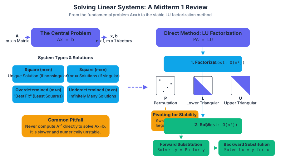
Root Finding for Nonlinear Equations
Key concepts: Root-Finding · Bisection Method · Fixed-Point Iteration · Newton's Method · Secant Method · Order of Convergence (Linear vs. Quadratic)
This section introduces iterative algorithms for solving nonlinear equations of the form f(x)=0, a common problem known as root-finding. It details and compares several fundamental methods, including the Bisection Method, Fixed-Point Iteration, Newton's Method, and the Secant Method. The focus is on understanding their mechanisms, convergence rates, and practical trade-offs.
Root Finding for Nonlinear Equations
In numerical analysis, while solving systems of linear equations of the form Ax = b is a well-defined and foundational problem, a vast array of challenges in science, engineering, and finance are inherently nonlinear. These problems require us to find the roots (or zeros) of a nonlinear function f(x), which are the values of x such that f(x) = 0. Unlike their linear counterparts, nonlinear equations rarely have a direct, analytical solution. Consequently, we must turn to iterative methods: algorithms that generate a sequence of improving approximations, x_0, x_1, x_2, ..., that—if all goes well—converge to the true root.
The choice of method involves a critical trade-off between speed, robustness, and the amount of information required about the function (such as its derivative). Understanding these algorithms is not just an academic exercise; it's fundamental to solving complex optimization, simulation, and modeling problems.
The Bisection Method: Slow but Steady
The Bisection Method is the simplest and most robust root-finding algorithm. Its reliability stems from a simple, powerful mathematical principle: the Intermediate Value Theorem.
What It Is
The Bisection Method is a bracketing method for finding a root of a continuous function
f(x). It begins with an interval[a, b]where the function values at the endpoints,f(a)andf(b), have opposite signs. The method repeatedly halves the interval while ensuring the root remains bracketed within the smaller interval.
The core requirement, f(a) * f(b) < 0, guarantees, by the Intermediate Value Theorem, that at least one root must exist within the interval (a, b).
Why It Matters
The primary virtue of the Bisection Method is its guaranteed convergence. As long as the initial interval brackets a root and the function is continuous, the method will converge to a root. This makes it an excellent fallback or a tool for obtaining a rough but reliable initial guess for a faster, less stable method. Its main drawback is its slow rate of convergence.
How It Works
The algorithm proceeds as follows:
- Initialization: Choose an interval
[a, b]such thatf(a)andf(b)have opposite signs. Define a tolerancetoland a maximum number of iterationsmax_iter. - Iteration: For
n = 1, 2, ...up tomax_iter: a. Calculate the midpoint:c = (a + b) / 2. b. Evaluatef(c). c. Check for convergence: If|f(c)| < tolor(b - a) / 2 < tol, the process has converged. Returnc. d. Update the interval: - Iff(a) * f(c) < 0, the root is in the left half. Setb = c. - Else, the root is in the right half. Seta = c. - Termination: If the loop finishes without converging, the method has failed (e.g.,
max_iterwas reached).
The width of the search interval is halved at each step. After n iterations, the width of the interval containing the root is (b_0 - a_0) / 2^n, where [a_0, b_0] is the initial interval.
Concrete Example
Let's find the root of f(x) = x^3 - x - 2 on the interval [1, 2].
- We know
f(1) = 1 - 1 - 2 = -2andf(2) = 8 - 2 - 2 = 4. Since the signs are opposite, a root is bracketed.
| Iteration (n) | a | b | c = (a+b)/2 | f(c) | New Interval | Interval Width |
|---|---|---|---|---|---|---|
| 1 | 1.0 | 2.0 | 1.5 | -0.125 | [1.5, 2.0] |
0.5 |
| 2 | 1.5 | 2.0 | 1.75 | 1.609375 | [1.5, 1.75] |
0.25 |
| 3 | 1.5 | 1.75 | 1.625 | 0.666016 | [1.5, 1.625] |
0.125 |
| 4 | 1.5 | 1.625 | 1.5625 | 0.252197 | [1.5, 1.5625] |
0.0625 |
| 5 | 1.5 | 1.5625 | 1.53125 | 0.059113 | [1.5, 1.53125] |
0.03125 |
The method slowly but surely closes in on the true root, which is approximately 1.521.
Implementation in Python
Here is a robust, low-level implementation of the Bisection Method in Python.
import math

def bisection_method(f, a, b, tol=1e-9, max_iter=100):
    """
    Finds a root of a function f within the interval [a, b] using the bisection method.

    Args:
        f (callable): The function for which to find a root.
        a (float): The left endpoint of the interval.
        b (float): The right endpoint of the interval.
        tol (float): The tolerance for convergence.
        max_iter (int): The maximum number of iterations.

    Returns:
        float: The approximate root.

    Raises:
        ValueError: If f(a) and f(b) do not have opposite signs.
    """
    fa = f(a)
    fb = f(b)

    if fa * fb >= 0:
        raise ValueError("Root not bracketed: f(a) and f(b) must have opposite signs.")

    for i in range(max_iter):
        c = a + (b - a) / 2  # Avoids potential overflow of (a+b)/2
        fc = f(c)

        # Check for convergence
        if abs(fc) < tol or (b - a) / 2 < tol:
            print(f"Converged after {i+1} iterations.")
            return c

        # Update the interval
        if fa * fc < 0:
            b = c
            fb = fc
        else:
            a = c
            fa = fc

    print(f"Failed to converge within {max_iter} iterations.")
    return c

# Example usage:
# Find the root of f(x) = x^3 - x - 2
root = bisection_method(lambda x: x**3 - x - 2, 1, 2)
print(f"Approximate root: {root:.8f}")
# Output:
# Converged after 30 iterations.
# Approximate root: 1.52137971
Common Pitfalls
- Finding the initial bracket
[a, b]: This can be a significant challenge. It often requires prior knowledge of the function or a graphical analysis. - Multiple roots: If the initial interval contains multiple roots, the bisection method will find one of them, but it's not predictable which one.
- Singularities: If the function has a singularity within the interval (e.g.,
f(x) = 1/xon[-1, 1]), the method can be misled and converge to the singularity instead of a root. - Roots of even multiplicity: The method fails for roots where the function touches the x-axis but doesn't cross it (e.g.,
f(x) = x^2atx=0), as it's impossible to find an interval[a, b]wheref(a)andf(b)have opposite signs.
Fixed-Point Iteration
Fixed-Point Iteration is a beautifully simple and general method that reframes the root-finding problem f(x) = 0 into a search for a fixed point, a point x such that x = g(x).
What It Is
A fixed point of a function
g(x)is a valuersuch thatr = g(r). Fixed-Point Iteration attempts to find such a point by generating the sequencex_{n+1} = g(x_n)starting from an initial guessx_0.
To apply this method, we must first algebraically rearrange our original equation f(x) = 0 into the form x = g(x). This rearrangement is not unique and is the most critical step in the process.
Why It Matters
This method provides a theoretical framework for understanding other iterative schemes, including Newton's Method. The convergence of the iteration depends entirely on the properties of the function g(x), specifically its derivative near the fixed point. This provides deep insight into why certain methods converge quickly while others diverge.
How It Works
- Rearrangement: Transform the equation
f(x) = 0into the formx = g(x). - Initialization: Choose an initial guess
x_0. - Iteration: Generate the sequence
x_{n+1} = g(x_n)until the difference|x_{n+1} - x_n|is smaller than a specified tolerance.
The success of the method hinges on the Contraction Mapping Theorem.
Fixed-Point Theorem (Simplified): If g is a continuous function on a closed interval [a, b] such that g(x) maps [a, b] to itself, and if its derivative satisfies |g'(x)| ≤ k < 1 for all x in (a, b), then:
- There exists a unique fixed point
rin[a, b]. - The iteration
x_{n+1} = g(x_n)will converge torfor any initial guessx_0in[a, b].
In essence, if the function g(x) is a "contraction" (its slope has a magnitude less than 1), it will always pull points closer to the fixed point.
Concrete Example
Let's solve f(x) = e^{-x} - x = 0. The root is where the graphs of y=x and y=e^{-x} intersect.
A natural rearrangement is x = e^{-x}. So, we define g(x) = e^{-x}.
Let's analyze the derivative: g'(x) = -e^{-x}. The root is around 0.5. Near this point, |g'(0.5)| = |-e^{-0.5}| ≈ 0.606 < 1. The condition is met, so the iteration should converge.
Let's start with x_0 = 0:
x_1 = g(x_0) = e^0 = 1x_2 = g(x_1) = e^{-1} ≈ 0.3678x_3 = g(x_2) = e^{-0.3678} ≈ 0.6922x_4 = g(x_3) = e^{-0.6922} ≈ 0.5004x_5 = g(x_4) = e^{-0.5004} ≈ 0.6062- ... This sequence converges (albeit slowly) to the true root
r ≈ 0.56714.
Derivation of Convergence
The condition |g'(x)| < 1 directly determines the convergence rate. We can prove this using the Mean Value Theorem. Let r be the fixed point, so r = g(r). The error at step n is e_n = x_n - r.
# Derivation of Linear Convergence for Fixed-Point Iteration

# Error at step n+1:
e_{n+1} = x_{n+1} - r
        = g(x_n) - g(r)

# By the Mean Value Theorem, there exists a c_n between x_n and r such that:
# g(x_n) - g(r) = g'(c_n) * (x_n - r)

# Substituting this back:
e_{n+1} = g'(c_n) * e_n

# Taking the absolute value:
|e_{n+1}| = |g'(c_n)| * |e_n|

# As n -> infinity, x_n -> r, and thus c_n -> r.
# Therefore, in the limit:
# |e_{n+1}| ≈ |g'(r)| * |e_n|

# This shows that the error is reduced by a constant factor |g'(r)| at each step.
# This is the definition of linear convergence, provided 0 < |g'(r)| < 1.
# If g'(r) = 0, convergence is faster (as we will see with Newton's Method).
Common Pitfalls
- Choice of
g(x): Everything depends on this. For a singlef(x) = 0, there are infinite ways to writex = g(x). A poor choice can lead to slow convergence or, worse, divergence. For example, rearrangingx^2 - 2 = 0tox = 2/xwould diverge for any initial guess other than the root itself. - Divergence: If
|g'(x)| > 1near the fixed point, each iteration will move the estimate further away from the root, causing the method to diverge rapidly.
Newton's Method (Newton-Raphson)
Newton's Method is arguably the most famous and powerful root-finding algorithm. It is an open method, meaning it does not require the root to be bracketed. When it works, its convergence is exceptionally fast.
What It Is
Newton's Method is an iterative algorithm that approximates a root of a differentiable function
f(x)by using the tangent line at the current estimate. The next approximation is taken as the x-intercept of this tangent line.
How It Works
The derivation is elegant and straightforward. Given a current guess x_n, the equation of the tangent line to the curve y = f(x) at the point (x_n, f(x_n)) is:
y - f(x_n) = f'(x_n) * (x - x_n)
To find the x-intercept, we set y = 0 and solve for x, which we will call our next guess, x_{n+1}:
0 - f(x_n) = f'(x_n) * (x_{n+1} - x_n)
Rearranging for x_{n+1} gives the celebrated Newton's iteration formula:
x_{n+1} = x_n - f(x_n) / f'(x_n)
The process begins with an initial guess x_0 and repeats this iteration until convergence.
Concrete Example
Let's find the square root of 9, which is equivalent to finding the positive root of f(x) = x^2 - 9 = 0.
- The function is
f(x) = x^2 - 9. - The derivative is
f'(x) = 2x. - The iteration formula is
x_{n+1} = x_n - (x_n^2 - 9) / (2x_n).
Let's start with a poor initial guess, x_0 = 1.
x_1 = 1 - (1^2 - 9) / (2*1) = 1 - (-8)/2 = 1 + 4 = 5x_2 = 5 - (5^2 - 9) / (2*5) = 5 - 16/10 = 5 - 1.6 = 3.4x_3 = 3.4 - (3.4^2 - 9) / (2*3.4) = 3.4 - (11.56 - 9) / 6.8 = 3.4 - 2.56 / 6.8 ≈ 3.0235x_4 = 3.0235 - (3.0235^2 - 9) / (2*3.0235) ≈ 3.00009
Notice how quickly the approximation approaches the true root 3. The number of correct digits roughly doubles with each iteration, a hallmark of quadratic convergence.
Real-World Usage with SciPy
In practice, you would rarely implement Newton's method from scratch. Instead, you would use a well-tested library function like scipy.optimize.newton.
# Using a library to find the root of f(x) = cos(x) - x
import numpy as np
from scipy.optimize import newton

# Define the function and its derivative
def f(x):
    return np.cos(x) - x

def f_prime(x):
    return -np.sin(x) - 1

# Initial guess
x0 = 0.5

# Use the newton function from SciPy, providing the function,
# initial guess, and the derivative (fprime).
# The library handles tolerance and iteration limits.
root = newton(f, x0, fprime=f_prime, tol=1.48e-08, maxiter=50)

print(f"The root is approximately: {root}")
print(f"Value of f at the root: {f(root)}")

# Output:
# The root is approximately: 0.7390851332151607
# Value of f at the root: 0.0
Common Pitfalls
- Requires the derivative: The need to compute
f'(x)can be a significant drawback if the derivative is complex or computationally expensive. - Divergence at
f'(x_n) = 0: If the iteration lands on a point where the tangent is horizontal, the denominator becomes zero, and the method fails catastrophically. - Poor initial guess: If
x_0is far from the actual root, the tangent line can shoot the next guess off to a distant region, leading to divergence or convergence to an unintended root. - Cycles: For some functions, the iteration can enter a cycle, bouncing between two or more values without ever converging.
The Secant Method: Newton's Practical Cousin
The Secant Method is a clever modification of Newton's Method that circumvents its most significant weakness: the need for an explicit derivative.
What It Is
The Secant Method is an iterative, open root-finding method that approximates the derivative in Newton's formula using a finite difference based on the two previous iterations. Instead of a tangent line, it uses a secant line.
How It Works
The derivative f'(x_n) is the slope of the tangent at x_n. We can approximate this slope using the two most recent points in our sequence, (x_{n-1}, f(x_{n-1})) and (x_n, f(x_n)):
f'(x_n) ≈ (f(x_n) - f(x_{n-1})) / (x_n - x_{n-1})
Substituting this approximation into Newton's formula gives the Secant Method iteration:
x_{n+1} = x_n - f(x_n) * (x_n - x_{n-1}) / (f(x_n) - f(x_{n-1}))
Notice that this method requires two initial guesses, x_0 and x_1, to begin.
Implementation in C
Here is a C implementation to illustrate the algorithm at a lower level.
#include <stdio.h>
#include <math.h>

// The function for which we are finding the root: f(x) = x^3 - x - 2
double func(double x) {
    return x*x*x - x - 2.0;
}

void secant_method(double x0, double x1, double tol, int max_iter) {
    double f0, f1, x2;
    int iter = 0;

    printf("Iter\t x_n\t\t f(x_n)\n");
    printf("----------------------------------------\n");

    for (iter = 0; iter < max_iter; ++iter) {
        f0 = func(x0);
        f1 = func(x1);

        if (fabs(f1 - f0) < 1e-12) { // Avoid division by zero
            printf("Denominator is too small. Method fails.\n");
            return;
        }

        x2 = x1 - f1 * (x1 - x0) / (f1 - f0);

        printf("%d\t %.8f\t %.8f\n", iter + 1, x2, func(x2));

        if (fabs(x2 - x1) < tol) {
            printf("\nConverged to root: %.10f\n", x2);
            return;
        }

        // Update points for the next iteration
        x0 = x1;
        x1 = x2;
    }

    printf("\nFailed to converge within %d iterations.\n", max_iter);
}

int main() {
    // Initial guesses for f(x) = x^3 - x - 2
    double x0 = 1.0;
    double x1 = 2.0;
    double tolerance = 1e-9;
    int max_iterations = 20;

    secant_method(x0, x1, tolerance, max_iterations);

    return 0;
}
Common Pitfalls
- Divergence: It shares the same sensitivity to the initial guess as Newton's method.
- Numerical Instability: If
x_nandx_{n-1}become very close,f(x_n)andf(x_{n-1})will also be very close. The denominatorf(x_n) - f(x_{n-1})can suffer from catastrophic cancellation, leading to a massive loss of precision. - Slower than Newton's: While much faster than bisection, its convergence rate is slightly less than Newton's.
Order of Convergence: A Deeper Look
The "speed" of an iterative method is formally characterized by its order of convergence. This tells us how quickly the error decreases from one iteration to the next.
An iterative method has an order of convergence
pif the errore_n = x_n - rsatisfies the relation:lim_{n→∞} |e_{n+1}| / |e_n|^p = Cfor some non-zero constantC(the asymptotic error constant).
Linear vs. Quadratic Convergence
-
Linear Convergence (
p=1):- The error is reduced by a roughly constant factor at each step:
|e_{n+1}| ≈ C * |e_n|. - For convergence, we must have
0 < C < 1. - This means the algorithm gains a constant number of correct digits per iteration.
- Examples: Bisection Method, Fixed-Point Iteration.
- The error is reduced by a roughly constant factor at each step:
-
Quadratic Convergence (
p=2):- The error is proportional to the square of the previous error:
|e_{n+1}| ≈ C * |e_n|^2. - Once the error
|e_n|becomes small (e.g.,10^{-k}), the next error will be much smaller (e.g.,10^{-2k}). - This means the number of correct digits doubles at each iteration, leading to extremely rapid convergence near the root.
- Example: Newton's Method (for simple roots).
- The error is proportional to the square of the previous error:
-
Super-linear Convergence (
1 < p < 2):- Faster than linear, but not as fast as quadratic.
- Example: The Secant Method has an order of convergence
p = φ ≈ 1.618(the golden ratio).
Method Comparison Summary
This table summarizes the key properties of the methods discussed.
| Method | Convergence Order (p) | Derivative Required? | Initial Guesses | Robustness | Key Feature |
|---|---|---|---|---|---|
| Bisection | Linear (p=1) | No | 2 (bracketing) | Guaranteed | Unbeatable reliability |
| Fixed-Point | Linear (p=1) | No (but g'(x) for analysis) |
1 | Depends on g(x) |
General theoretical framework |
| Newton's | Quadratic (p=2) | Yes (f'(x)) |
1 | Can diverge | Extremely fast convergence |
| Secant | Super-linear (p≈1.618) | No | 2 | Can diverge | A practical, derivative-free Newton's |
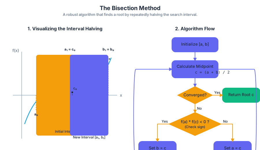
Polynomial Interpolation and Approximation
Key concepts: Polynomial Interpolation · Monomial Basis · Lagrange Basis · Newton Basis · Horner's Method · Piecewise Interpolation · Interpolation Error · Chebyshev Points
This section covers techniques for constructing polynomials that pass through a given set of data points. It explores different bases for representing these polynomials, including the Monomial, Lagrange, and Newton bases, and analyzes their computational efficiency. The material also touches on piecewise interpolation and the use of Chebyshev points to minimize error.
Polynomial Interpolation and Approximation
In numerical analysis and applied mathematics, we are frequently confronted with a set of discrete data points—perhaps from a physical experiment, a simulation, or the sampling of a complex function—and need to model the underlying relationship. Polynomial interpolation is a fundamental technique for constructing a continuous function, specifically a polynomial, that passes exactly through a given set of data points. This process creates a simple, smooth, and easily differentiable model from discrete information.
However, the quest for the "best" interpolating polynomial is nuanced. While a unique polynomial of a certain degree is guaranteed to exist for any non-degenerate set of points, the way we represent and compute this polynomial has profound implications for numerical stability, computational efficiency, and the accuracy of the approximation between the given points. This section provides a deep dive into the theory, methods, and practical trade-offs of polynomial interpolation.
The Interpolation Problem: Existence and Uniqueness
Before exploring various methods, let's formally define the problem and state the foundational theorem that guarantees our efforts are not in vain.
The Polynomial Interpolation Problem: Given a set of
n+1distinct data points(x_0, y_0), (x_1, y_1), ..., (x_n, y_n)where allx_iare unique, find a polynomialp(x)of degree at mostnsuch thatp(x_i) = y_ifor alli = 0, 1, ..., n.
This problem always has a solution, and that solution is unique.
Theorem: Existence and Uniqueness of the Interpolating Polynomial For any set of
n+1data points(x_i, y_i)with distinctx_i, there exists a unique polynomialp_n(x)of degree at mostnthat satisfies the interpolation conditionsp_n(x_i) = y_ifor alli.
This theorem is the bedrock of our work. It assures us that no matter which method we choose to find the polynomial—Monomial, Lagrange, or Newton form—we are ultimately finding different representations of the same unique mathematical object. The choice of method is therefore not about finding a different answer, but about finding the same answer in a way that is computationally efficient, numerically stable, and adaptable to our needs.
The Monomial Basis: A Natural but Flawed Approach
The most straightforward way to represent a polynomial is in the monomial basis, {1, x, x², ..., xⁿ}. This is the form we learn in introductory algebra.
What It Is
An n-degree polynomial p(x) in the monomial basis is written as:
p(x) = c_0 + c_1x + c_2x^2 + ... + c_nx^n
The interpolation task is to find the coefficients c_0, c_1, ..., c_n such that p(x_i) = y_i for all our data points.
How It Works
Substituting each data point (x_i, y_i) into the polynomial equation gives us a system of n+1 linear equations for the n+1 unknown coefficients c_j:
c_0 + c_1x_0 + c_2x_0^2 + ... + c_nx_0^n = y_0
c_0 + c_1x_1 + c_2x_1^2 + ... + c_nx_1^n = y_1
...
c_0 + c_1x_n + c_2x_n^2 + ... + c_nx_n^n = y_n
This system can be written in matrix form as Vc = y, where c is the vector of unknown coefficients, y is the vector of y_i values, and V is a special matrix known as the Vandermonde matrix.
\begin{pmatrix}
1 & x_0 & x_0^2 & \cdots & x_0^n \\
1 & x_1 & x_1^2 & \cdots & x_1^n \\
\vdots & \vdots & \vdots & \ddots & \vdots \\
1 & x_n & x_n^2 & \cdots & x_n^n
\end{pmatrix}
\begin{pmatrix}
c_0 \\
c_1 \\
\vdots \\
c_n
\end{pmatrix}
=
\begin{pmatrix}
y_0 \\
y_1 \\
\vdots \\
y_n
\end{pmatrix}
To find the coefficients, we simply need to solve this linear system for c.
Concrete Example
Let's find the quadratic polynomial that passes through the points (1, 1), (2, 4), and (3, 3). Here, n=2.
The Vandermonde system is:
V = [[1, 1, 1], [1, 2, 4], [1, 3, 9]]
y = [1, 4, 3]
The system of equations is:
c_0 + 1c_1 + 1c_2 = 1
c_0 + 2c_1 + 4c_2 = 4
c_0 + 3c_1 + 9c_2 = 3
Solving this system (e.g., using Gaussian elimination or a library function) yields c = [-4, 6.5, -1.5].
Thus, the interpolating polynomial is p(x) = -1.5x² + 6.5x - 4.
Implementation in Python
Solving a Vandermonde system is a standard task in numerical computing. Here is a Python implementation using NumPy.
import numpy as np

def monomial_interpolation_coeffs(x_points, y_points):
    """
    Computes the coefficients of the interpolating polynomial in the monomial basis.

    Args:
        x_points (np.ndarray): Array of x-coordinates of the data points.
        y_points (np.ndarray): Array of y-coordinates of the data points.

    Returns:
        np.ndarray: The coefficient vector [c_0, c_1, ..., c_n].
    """
    if len(x_points) != len(y_points):
        raise ValueError("x_points and y_points must have the same length.")

    n = len(x_points) - 1
    # np.vander creates the Vandermonde matrix with columns [x^n, x^(n-1), ..., 1]
    # We flip it to match our definition [1, x, ..., x^n]
    V = np.vander(x_points, increasing=True)

    # Solve the linear system Vc = y
    try:
        coeffs = np.linalg.solve(V, y_points)
        return coeffs
    except np.linalg.LinAlgError:
        raise RuntimeError("The Vandermonde matrix is singular. Check if x_points are distinct.")

# Example from the text
x_pts = np.array([1., 2., 3.])
y_pts = np.array([1., 4., 3.])

coeffs = monomial_interpolation_coeffs(x_pts, y_pts)
print(f"Coefficients (c0, c1, c2): {coeffs}") # Expected: [-4. ,  6.5, -1.5]

# To verify, let's evaluate the polynomial at x=2
p_at_2 = coeffs[0] + coeffs[1]*2 + coeffs[2]*2**2
print(f"p(2) = {p_at_2}") # Expected: 4.0
Common Pitfalls
The primary drawback of the monomial basis is numerical instability. For a high number of points, or for points clustered closely together, the Vandermonde matrix becomes ill-conditioned. An ill-conditioned matrix is one where small changes in the input y can lead to very large changes in the output solution c. This is because the columns of V, which are powers of x, become nearly linearly dependent for large n. The condition number of the matrix grows exponentially with n, making the solution highly sensitive to floating-point errors.
In practice, direct solution of the Vandermonde system is rarely used for n > 10.
The Lagrange Basis: An Elegant Theoretical Tool
The Lagrange basis offers a brilliantly clever way to construct the interpolating polynomial, completely bypassing the need to solve a linear system.
What It Is
The Lagrange basis consists of a set of n+1 polynomials, L_0(x), L_1(x), ..., L_n(x), each of degree n. These basis polynomials are defined with a special property related to the data points x_i.
Definition: Lagrange Basis Polynomials Each Lagrange basis polynomial
L_j(x)is defined as:L_j(x) = Π_{i=0, i≠j}^{n} (x - x_i) / (x_j - x_i)These polynomials have the "Kronecker delta" property:
L_j(x_k) = 1ifj=kand0ifj≠k.
How It Works
With this property, constructing the final interpolating polynomial p(x) becomes trivial. We form a linear combination of these basis polynomials, where the coefficients are simply the y_i values of our data points.
p(x) = Σ_{j=0}^{n} y_j * L_j(x)
Let's verify this works. If we evaluate p(x) at some x_k:
p(x_k) = Σ_{j=0}^{n} y_j * L_j(x_k)
Because L_j(x_k) is zero for all j≠k and one for j=k, all terms in the sum disappear except for one:
p(x_k) = y_k * L_k(x_k) = y_k * 1 = y_k
The polynomial passes through all points by construction.
Concrete Example
Using the same points (1, 1), (2, 4), (3, 3). Here x_0=1, x_1=2, x_2=3 and y_0=1, y_1=4, y_2=3.
- Construct
L_0(x):L_0(x) = ((x-x_1)(x-x_2)) / ((x_0-x_1)(x_0-x_2)) = ((x-2)(x-3)) / ((1-2)(1-3)) = (x²-5x+6)/2 - Construct
L_1(x):L_1(x) = ((x-x_0)(x-x_2)) / ((x_1-x_0)(x_1-x_2)) = ((x-1)(x-3)) / ((2-1)(2-3)) = (x²-4x+3)/(-1) - Construct
L_2(x):L_2(x) = ((x-x_0)(x-x_1)) / ((x_2-x_0)(x_2-x_1)) = ((x-1)(x-2)) / ((3-1)(3-2)) = (x²-3x+2)/2
The final polynomial is p(x) = y_0*L_0(x) + y_1*L_1(x) + y_2*L_2(x):
p(x) = 1 * (x²-5x+6)/2 + 4 * -(x²-4x+3) + 3 * (x²-3x+2)/2
Expanding and collecting terms gives p(x) = -1.5x² + 6.5x - 4, the same polynomial we found earlier.
Implementation in C
Here's a C function to evaluate a Lagrange polynomial at a specific point. This low-level implementation highlights the nested loop structure inherent in the formula.
#include <stdio.h>

// Evaluates the Lagrange interpolating polynomial at a single point 'x'.
double lagrange_evaluate(double x, const double* x_points, const double* y_points, int n) {
    double result = 0.0;

    // Outer loop for the sum: Σ y_j * L_j(x)
    for (int j = 0; j < n; ++j) {
        // Inner loop to compute L_j(x)
        double l_j = 1.0;
        for (int i = 0; i < n; ++i) {
            if (i != j) {
                l_j *= (x - x_points[i]) / (x_points[j] - x_points[i]);
            }
        }
        result += y_points[j] * l_j;
    }
    return result;
}

int main() {
    double x_pts[] = {1.0, 2.0, 3.0};
    double y_pts[] = {1.0, 4.0, 3.0};
    int n = sizeof(x_pts) / sizeof(x_pts[0]);

    // Evaluate at a few points to test
    printf("p(1.0) = %f\n", lagrange_evaluate(1.0, x_pts, y_pts, n)); // Expected: 1.0
    printf("p(2.0) = %f\n", lagrange_evaluate(2.0, x_pts, y_pts, n)); // Expected: 4.0
    printf("p(2.5) = %f\n", lagrange_evaluate(2.5, x_pts, y_pts, n)); // Expected: 4.375

    return 0;
}
Pitfalls and Variations
The main drawbacks of the Lagrange form are:
- Costly Evaluation: A naive evaluation, as shown in the C code, takes
O(n²)operations for each pointx. - Static Nature: If a new data point
(x_{n+1}, y_{n+1})is added, all Lagrange basis polynomials must be recomputed from scratch.
A significant improvement is the Barycentric Interpolation Formula, which is an algebraic rearrangement of the Lagrange form. It allows evaluation in O(n) time after an initial O(n²) pre-computation of weights. This makes it much more practical for repeated evaluations.
The Newton Basis: Efficient and Incremental
The Newton basis strikes a balance, offering both efficient evaluation and an elegant, incremental way to build the polynomial. It is often the most practical choice.
What It Is
The Newton form of the interpolating polynomial is:
p(x) = a_0 + a_1(x-x_0) + a_2(x-x_0)(x-x_1) + ... + a_n(x-x_0)...(x-x_{n-1})
The basis polynomials are π_j(x) = Π_{i=0}^{j-1} (x-x_i). The challenge is to find the coefficients a_0, a_1, ..., a_n.
How It Works: Divided Differences
The coefficients a_k are found using a recursive method called divided differences.
Definition: Divided Differences
- Zeroth divided difference:
f[x_i] = y_i - First divided difference:
f[x_i, x_{i+1}] = (f[x_{i+1}] - f[x_i]) / (x_{i+1} - x_i) - k-th divided difference:
f[x_i, ..., x_{i+k}] = (f[x_{i+1}, ..., x_{i+k}] - f[x_i, ..., x_{i+k-1}]) / (x_{i+k} - x_i)
The coefficients of the Newton polynomial are the top diagonal of the divided differences table:
a_k = f[x_0, x_1, ..., x_k]
This computation is typically organized in a triangular table.
Concrete Example
Let's use a new set of 4 points for clarity: (0, 1), (1, 4), (3, 40), (4, 85).
We build the divided differences table:
x_i |
f[x_i] (a₀) |
f[x_i, x_{i+1}] (a₁) |
f[x_i, ..., x_{i+2}] (a₂) |
f[x_i, ..., x_{i+3}] (a₃) |
|---|---|---|---|---|
| 0 | 1 | |||
(4-1)/(1-0) = 3 |
||||
| 1 | 4 | (18-3)/(3-0) = 5 |
||
(40-4)/(3-1) = 18 |
(7-5)/(4-0) = 0.5 |
|||
| 3 | 40 | (45-18)/(4-1) = 9 |
||
(85-40)/(4-3) = 45 |
||||
| 4 | 85 |
The coefficients are the top entries: a_0=1, a_1=3, a_2=5, a_3=0.5.
The polynomial is:
p(x) = 1 + 3(x-0) + 5(x-0)(x-1) + 0.5(x-0)(x-1)(x-3)
Algorithm and Library Usage
The process of computing the divided differences is algorithmic.
function DividedDifferences(x_points, y_points):
    n = length(x_points)
    // Initialize a table (e.g., a 2D array)
    table = new array of size n x n

    // The first column is just the y-values
    for i from 0 to n-1:
        table[i][0] = y_points[i]

    // Compute the rest of the table
    for j from 1 to n-1: // Column index
        for i from 0 to n-1-j: // Row index
            numerator = table[i+1][j-1] - table[i][j-1]
            denominator = x_points[i+j] - x_points[i]
            table[i][j] = numerator / denominator

    // The coefficients are the first row of the table
    return table[0]
In practice, high-quality numerical libraries provide robust implementations. SciPy's BarycentricInterpolator uses a related form and can be updated efficiently.
import numpy as np
from scipy.interpolate import BarycentricInterpolator
import matplotlib.pyplot as plt

# Data points
xi = np.array([0., 1., 3., 4.])
yi = np.array([1., 4., 40., 85.])

# Create the interpolator object
poly = BarycentricInterpolator(xi, yi)

# Let's add a new point to demonstrate the incremental nature
# This is a key advantage of Newton-like forms
new_x, new_y = 2.0, 15.0
poly.add_xi(np.array([new_x]), np.array([new_y]))

# Generate points for plotting a smooth curve
x_dense = np.linspace(-0.5, 4.5, 400)
y_dense = poly(x_dense)

# Plot the results
plt.style.use('seaborn-v0_8-whitegrid')
plt.figure(figsize=(10, 6))
plt.plot(x_dense, y_dense, label='Newton Interpolating Polynomial (with added point)')
plt.plot(xi, yi, 'ro', label='Original Points')
plt.plot(new_x, new_y, 'go', markersize=10, label='Added Point (2, 15)')
plt.title('Newton Interpolation with Incremental Update')
plt.xlabel('x')
plt.ylabel('y')
plt.legend()
plt.show()
Efficient Polynomial Evaluation: Horner's Method
Regardless of how we find the coefficients c_i for the monomial form p(x) = c_0 + c_1x + ... + c_nx^n, evaluating it efficiently is critical. A naive evaluation requires O(n²) multiplications (computing x^k for each term). Horner's Method is an elegant algorithm that reduces this to O(n).
How It Works
Horner's method works by refactoring the polynomial into a nested form. For a degree 4 polynomial:
p(x) = c_0 + c_1x + c_2x² + c_3x³ + c_4x⁴
p(x) = c_0 + x(c_1 + x(c_2 + x(c_3 + x(c_4))))
This nested structure can be evaluated from the inside out with a simple loop, requiring only n multiplications and n additions.
Implementation in JavaScript
This algorithm is simple and efficient, making it suitable for implementation in any language. Here's a JavaScript example.
/**
 * Evaluates a polynomial in monomial form using Horner's method.
 * @param {number[]} coeffs - Array of coefficients [c0, c1, ..., cn].
 * @param {number} x - The point at which to evaluate the polynomial.
 * @returns {number} The value of the polynomial at x.
 */
function horner(coeffs, x) {
    // Start with the highest-degree coefficient
    let result = coeffs[coeffs.length - 1];

    // Iterate backwards from the second to last coefficient
    for (let i = coeffs.length - 2; i >= 0; i--) {
        result = result * x + coeffs[i];
    }

    return result;
}

// Example: p(x) = -1.5x² + 6.5x - 4  (coeffs are [-4, 6.5, -1.5])
const myCoeffs = [-4, 6.5, -1.5];
console.log(`p(1) = ${horner(myCoeffs, 1)}`); // Expected: 1
console.log(`p(2) = ${horner(myCoeffs, 2)}`); // Expected: 4
console.log(`p(3) = ${horner(myCoeffs, 3)}`); // Expected: 3
The Problem with High-Degree Polynomials: Runge's Phenomenon
A common misconception is that using more data points (and thus a higher-degree polynomial) will always lead to a better approximation of the underlying function. This is dangerously false. High-degree polynomial interpolants can exhibit wild oscillations, especially near the ends of the interpolation interval.
This behavior is known as Runge's phenomenon, famously demonstrated with the function f(x) = 1 / (1 + 25x²). When interpolating this function on the interval [-1, 1] with equally spaced points, the error between the true function and the interpolating polynomial p_n(x) grows dramatically as n increases.
The error of polynomial interpolation is given by:
f(x) - p_n(x) = (f^(n+1)(ξ) / (n+1)!) * Π_{i=0}^{n} (x - x_i)
where ξ is some point in the interval.
Two factors contribute to Runge's phenomenon:
- The derivatives of Runge's function grow very rapidly.
- The product term
Π(x - x_i)becomes very large near the endpoints for equally spaced points.
Solution: Chebyshev Points
The magnitude of the error can be controlled by changing the locations of the x_i points. The optimal choice to minimize the maximum error are the Chebyshev points, which are clustered more densely near the ends of the interval.
They are defined on [-1, 1] as:
x_i = cos( (2i+1)π / (2n+2) ) for i = 0, ..., n.
Using Chebyshev points instead of equispaced points dramatically mitigates Runge's phenomenon and guarantees convergence for a wide class of functions.
Piecewise Interpolation: The Practical Solution
Instead of using a single, high-degree polynomial to fit all data points, a more robust and widely used approach is piecewise interpolation. The idea is to divide the interval into smaller subintervals and fit a separate, low-degree polynomial on each piece. The collection of these polynomials is called a spline.
How It Works
- Piecewise Linear Interpolation: Simply connect consecutive data points with straight lines. The resulting function is continuous (
C⁰) but has sharp corners (its derivative is not continuous). - Piecewise Cubic Splines: The most common choice. We fit a cubic polynomial between each pair of points
(x_i, y_i)and(x_{i+1}, y_{i+1}). To ensure smoothness, we add constraints that the first and second derivatives must match at the "knots" (the data points). This results in a function that is twice continuously differentiable (C²), making it visually smooth and well-behaved.
Why It Matters
Splines avoid Runge's phenomenon entirely because they only ever use low-degree polynomials. They are stable, efficient to compute, and provide excellent approximations for most real-world data. They are the workhorse of interpolation in computer graphics, data visualization, and scientific computing.
| Method Comparison | Construction Cost | Evaluation Cost | Stability | Key Feature |
|---|---|---|---|---|
| Monomial Basis | O(n³) |
O(n) |
Poor | Simple representation, but ill-conditioned. |
| Lagrange Basis | O(n²) |
O(n²) |
Fair | Trivial coefficients, theoretically elegant. |
| Newton Basis | O(n²) |
O(n) |
Good | Incremental updates, numerically stable. |
| Cubic Splines | O(n) |
O(log n) |
Excellent | Avoids oscillations, provides C² smoothness. |
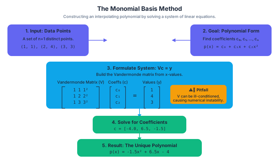
Midterm 2: Review and Assessment
Key concepts: Root-Finding Methods (Newton's, Secant, Bisection) · Convergence Analysis · Polynomial Interpolation (Lagrange, Vandermonde, Newton) · Interpolation Error Analysis · Piecewise vs. Global Interpolation
This module provides a comprehensive review for the second midterm, focusing on root-finding and polynomial interpolation. It includes a practice exam and solutions that test the theoretical understanding and practical application of methods like Newton's, Secant, and various interpolation techniques (Lagrange, Vandermonde, piecewise). Key concepts like convergence rates and error analysis are heavily featured.
Midterm 2: Review and Assessment
This module provides a comprehensive technical review for the second midterm, focusing on the core numerical methods of root-finding and polynomial interpolation. The exam will probe not only your ability to execute these algorithms but also your deeper understanding of their underlying mathematical principles, convergence properties, and the trade-offs that guide their application in real-world scenarios. Mastering these topics requires moving beyond rote memorization to a fluent understanding of why each method behaves as it does.
This guide is structured to mirror the conceptual flow of the course, from finding solutions to single nonlinear equations to approximating complex functions with simpler ones. We will dissect each major algorithm, analyze its performance characteristics, and work through practical examples to solidify your knowledge.
Root-Finding Methods: Seeking f(x) = 0
At its core, root-finding is the process of finding a value x (a root or zero) for which a given function f(x) evaluates to zero. This seemingly simple problem is fundamental across computational science and engineering, appearing in optimization problems (where we find the root of the derivative), equilibrium calculations, and solving systems of nonlinear equations. The midterm will focus on three canonical iterative methods.
The Bisection Method: The Reliable Bracket
-
What it is: The Bisection Method is a bracketing method that iteratively narrows down an interval
[a, b]that is known to contain a root. Its operation is guaranteed by the Intermediate Value Theorem, which states that if a continuous functionf(x)has values of opposite sign at the endpoints of an interval (i.e.,f(a) * f(b) < 0), then it must have at least one root within that interval. -
Why it matters: Its primary virtue is its unconditional convergence. As long as the initial bracket is valid, the Bisection Method is guaranteed to find a root. This makes it an incredibly robust and reliable algorithm, often used as a fallback or to generate a safe starting point for faster, but less reliable, methods.
-
How it works:
- Start with an interval
[a, b]such thatf(a)andf(b)have opposite signs. - Calculate the midpoint
c = (a + b) / 2. - Evaluate
f(c). - If
f(c)is sufficiently close to zero,cis the approximate root. - Otherwise, update the bracket:
- If
f(a) * f(c) < 0, the root is in[a, c]. Setb = c. - If
f(b) * f(c) < 0, the root is in[c, b]. Seta = c.
- If
- Repeat from step 2 until the interval
|b - a|is smaller than a specified tolerance.
- Start with an interval
-
Convergence Analysis: The Bisection Method exhibits linear convergence. At each step, the size of the interval containing the root is halved. If
e_nis the error at iterationn(represented by the interval width), thene_{n+1} = 0.5 * e_n. This is a constant factor reduction, which defines linear convergence. While reliable, this is considered slow compared to other methods.
Key Insight: The number of iterations
nrequired to achieve a toleranceεfrom an initial interval[a_0, b_0]can be calculated directly:n ≥ log₂((b_0 - a_0) / ε)This predictability is a unique and powerful feature of the Bisection Method.
- Common Pitfalls:
- Finding a valid initial bracket: For some functions, it can be difficult to find an initial
[a, b]wheref(a)andf(b)have opposite signs. - Multiple roots: If multiple roots exist in the initial bracket, Bisection will find one of them, but it's not predictable which one.
- Performance: Its slow, linear convergence makes it impractical for problems requiring high precision quickly.
- Finding a valid initial bracket: For some functions, it can be difficult to find an initial
Newton's Method: The Tangent Line Approximation
- What it is: Newton's Method (or Newton-Raphson) is an open method that uses tangent lines to iteratively find better approximations to a root. Starting with an initial guess
x_0, it approximates the functionf(x)with its tangent line atx_0and finds where this line intersects the x-axis. This intersection point becomes the next guess,x_1.
The iteration formula is derived from the first-order Taylor expansion of
f(x)aroundx_n:f(x) ≈ f(x_n) + f'(x_n)(x - x_n)Settingf(x) = 0to find the root and solving forx(which becomesx_{n+1}) gives the celebrated formula:x_{n+1} = x_n - f(x_n) / f'(x_n)
-
Why it matters: Speed. When Newton's Method converges, it typically does so extremely fast. This rapid convergence makes it the method of choice for a vast number of applications where efficiency is paramount.
-
How it works:
- Start with an initial guess
x_0that is "reasonably close" to the root. - Calculate the next approximation using the formula
x_{n+1} = x_n - f(x_n) / f'(x_n). - Repeat step 2 until the change
|x_{n+1} - x_n|or the residual|f(x_{n+1})|is below a tolerance.
- Start with an initial guess
Concrete Example: Find the root of f(x) = x² - 2 (i.e., find √2) starting with x_0 = 1.
* f'(x) = 2x
* Iteration 1: x_1 = 1 - (1² - 2) / (2 * 1) = 1 - (-1) / 2 = 1.5
* Iteration 2: x_2 = 1.5 - (1.5² - 2) / (2 * 1.5) = 1.5 - (0.25) / 3 ≈ 1.41667
* Iteration 3: x_3 = 1.41667 - (1.41667² - 2) / (2 * 1.41667) ≈ 1.4142157
The true value of √2 is 1.41421356.... Notice how the number of correct digits roughly doubles with each iteration.
- Convergence Analysis: Newton's Method has quadratic convergence under ideal conditions (the root is simple,
f'(r) ≠ 0, and the initial guess is sufficiently close). This means the errore_{n+1}is proportional to the square of the previous error:e_{n+1} ≈ C * e_n². This is the source of its incredible speed.
import math

def newtons_method(f, df, x0, tol=1e-9, max_iter=100):
    """
    Finds a root of a function using Newton's method.

    Args:
        f (callable): The function for which to find a root, f(x).
        df (callable): The derivative of the function, f'(x).
        x0 (float): Initial guess for the root.
        tol (float): The convergence tolerance.
        max_iter (int): The maximum number of iterations.

    Returns:
        float: The approximate root, or None if the method fails to converge.
    """
    x = x0
    for i in range(max_iter):
        fx = f(x)
        if abs(fx) < tol:
            print(f"Converged after {i} iterations.")
            return x

        dfx = df(x)
        if dfx == 0:
            print("Error: Derivative is zero. Newton's method fails.")
            return None

        x_new = x - fx / dfx

        if abs(x_new - x) < tol:
            print(f"Converged after {i+1} iterations.")
            return x_new

        x = x_new

    print("Warning: Maximum iterations reached. Did not converge.")
    return None

# Example usage: find the root of cos(x) - x^3
f = lambda x: math.cos(x) - x**3
df = lambda x: -math.sin(x) - 3*x**2
root = newtons_method(f, df, x0=0.5)
if root is not None:
    print(f"The root is approximately: {root:.8f}")
    print(f"f(root) = {f(root):.2e}")
# Derivation of Quadratic Convergence for Newton's Method

Let r be the true root, so f(r) = 0. Let e_n = x_n - r be the error at iteration n.
We use a Taylor expansion of f(r) around x_n:
  f(r) = f(x_n) + f'(x_n)(r - x_n) + (f''(ξ_n)/2)(r - x_n)²
  0    = f(x_n) - f'(x_n)e_n + (f''(ξ_n)/2)e_n²

Divide by f'(x_n) (assuming f'(x_n) ≠ 0):
  0 = f(x_n)/f'(x_n) - e_n + (f''(ξ_n)/(2f'(x_n)))e_n²

Rearrange to isolate the term f(x_n)/f'(x_n):
  f(x_n)/f'(x_n) = e_n - (f''(ξ_n)/(2f'(x_n)))e_n²

Now, look at the error in the next step, e_{n+1}:
  e_{n+1} = x_{n+1} - r
          = (x_n - f(x_n)/f'(x_n)) - r
          = (x_n - r) - f(x_n)/f'(x_n)
          = e_n - f(x_n)/f'(x_n)

Substitute the expression for f(x_n)/f'(x_n) from above:
  e_{n+1} = e_n - [e_n - (f''(ξ_n)/(2f'(x_n)))e_n²]
  e_{n+1} = (f''(ξ_n)/(2f'(x_n)))e_n²

As x_n approaches r, ξ_n also approaches r. So for large n:
  e_{n+1} ≈ [f''(r)/(2f'(r))] * e_n²

This shows that e_{n+1} is proportional to e_n², which is the definition of quadratic convergence.
The constant C is f''(r) / (2f'(r)).
- Common Pitfalls:
- Divergence: If the initial guess
x_0is not in the "basin of attraction" for the root, the iterations can diverge to infinity. - Zero Derivative: If
f'(x_n)is zero or very close to it, the next step will be huge or cause a division-by-zero error. This happens at local extrema. - Oscillation: The method can get stuck in a cycle between two or more points without converging.
- Requirement of
f'(x): The analytical derivative must be known and easy to compute, which is not always the case.
- Divergence: If the initial guess
The Secant Method: The Finite-Difference Newton
- What it is: The Secant Method is a clever modification of Newton's Method that avoids the need for an explicit derivative. It approximates the derivative
f'(x_n)using a finite difference based on the two most recent iterates,x_nandx_{n-1}.
The derivative approximation is:
f'(x_n) ≈ (f(x_n) - f(x_{n-1})) / (x_n - x_{n-1})Substituting this into Newton's formula gives the Secant iteration:x_{n+1} = x_n - f(x_n) * (x_n - x_{n-1}) / (f(x_n) - f(x_{n-1}))
-
Why it matters: It provides a practical alternative when the derivative is unavailable or computationally expensive. It almost achieves the speed of Newton's method without its main implementation burden.
-
How it works:
- Start with two initial guesses,
x_0andx_1. - Calculate the next approximation
x_{n+1}using the iteration formula. - Repeat, always using the two most recent points, until convergence is achieved.
- Start with two initial guesses,
-
Convergence Analysis: The Secant Method has superlinear convergence. Its rate is approximately
φ = (1 + √5) / 2 ≈ 1.618(the golden ratio). This meanse_{n+1} ≈ C * e_n^1.618. This is faster than linear but slower than quadratic. In practice, since it only requires one function evaluation per step (compared to two for Newton:fandf'), it can sometimes be faster in terms of wall-clock time. -
Common Pitfalls:
- Requires two initial points.
- It inherits many of the same potential divergence issues as Newton's method, as it is essentially a close approximation.
- If
f(x_n)becomes very close tof(x_{n-1}), the denominator can become small, leading to numerical instability (a form of subtractive cancellation).
Method Comparison
| Feature | Bisection Method | Newton's Method | Secant Method |
|---|---|---|---|
| Convergence Rate | Linear (p=1) |
Quadratic (p=2) |
Superlinear (p≈1.618) |
| Reliability | Guaranteed if bracket is valid | Can diverge | Can diverge |
| Requirements | [a, b] with f(a)f(b)<0 |
f(x), f'(x), and a good x₀ |
f(x) and two initial points x₀, x₁ |
| Cost per Iteration | 1 f evaluation |
1 f eval, 1 f' eval |
1 f evaluation |
| Key Advantage | Robustness & Predictability | Speed | No derivative needed |
| Key Disadvantage | Slow | Needs derivative, can fail | Needs two points, can fail |
Polynomial Interpolation: Connecting the Dots
Polynomial Interpolation is the task of finding a polynomial that passes exactly through a given set of data points. Given n+1 points (x_0, y_0), (x_1, y_1), ..., (x_n, y_n) with distinct x_i, we seek a unique polynomial P_n(x) of degree at most n such that P_n(x_i) = y_i for all i. The choice of basis for representing this polynomial leads to different algorithms with distinct computational trade-offs.
The Vandermonde Approach (Monomial Basis)
- What it is: This is the most direct approach. We assume the polynomial is in the standard monomial basis:
P_n(x) = c_0 + c_1x + c_2x² + ... + c_nx^n. Plugging in each data point(x_i, y_i)creates a system ofn+1linear equations for then+1unknown coefficientsc_j.
This system can be written in matrix form as
Vc = y:[ 1 x₀ x₀² ... x₀ⁿ ] [ c₀ ] [ y₀ ][ 1 x₁ x₁² ... x₁ⁿ ] [ c₁ ] = [ y₁ ][ ... ... ... ... ... ] [ .. ] [ .. ][ 1 xₙ xₙ² ... xₙⁿ ] [ cₙ ] [ yₙ ]The matrixVis the famous Vandermonde matrix.
-
Why it matters: It's a conceptually straightforward way to prove that a unique interpolating polynomial exists (since the Vandermonde matrix is invertible for distinct
x_i). However, it is rarely used in practice due to its severe numerical limitations. -
Pitfalls: The Vandermonde matrix is notoriously ill-conditioned, especially for high degrees and/or clustered points. This means that small errors in the input
y_ican lead to huge errors in the computed coefficientsc_j. Solving the systemVc=yis also computationally expensive, requiringO(n³)operations.
import numpy as np

# Data points to interpolate
x_vals = np.array([0, 1, 3, 4])
y_vals = np.array([2, 1, 5, 3])

# Build the Vandermonde matrix
V = np.vander(x_vals, increasing=True)
print("Vandermonde Matrix V:\n", V)

# Solve the linear system Vc = y for the coefficients c
try:
    coeffs = np.linalg.solve(V, y_vals)
    print("\nCoefficients (c0, c1, c2, c3):", coeffs)

    # Create a polynomial function from the coefficients
    p = np.poly1d(np.flip(coeffs)) # np.poly1d expects coeffs in decreasing power order
    print("\nInterpolating Polynomial P(x):\n", p)

except np.linalg.LinAlgError:
    print("\nCould not solve the system. The Vandermonde matrix may be singular or ill-conditioned.")

# A real-world library call for interpolation often uses a more stable basis internally.
# For example, using SciPy's BarycentricInterpolator which is related to Lagrange.
from scipy.interpolate import BarycentricInterpolator

poly_bary = BarycentricInterpolator(x_vals, y_vals)
print(f"\nValue at x=2 (using a stable library method): {poly_bary(2.0)}")
The Lagrange Basis
- What it is: The Lagrange approach constructs the polynomial differently. Instead of solving for coefficients, it builds the final polynomial as a weighted sum of special Lagrange basis polynomials,
L_j(x).
The interpolating polynomial is
P_n(x) = Σ_{j=0}^{n} y_j * L_j(x), where eachL_j(x)is a polynomial of degreenwith the property thatL_j(x_i) = 1ifi=jand0ifi≠j.L_j(x) = Π_{i=0, i≠j}^{n} (x - x_i) / (x_j - x_i)
-
Why it matters: It provides an elegant, explicit formula for the interpolating polynomial without needing to solve a linear system. The "coefficients" are simply the
y_ivalues themselves. -
Pitfalls:
- Evaluation is expensive: Evaluating
P_n(x)at a new point takesO(n²)operations. - Not adaptive: If a new data point
(x_{n+1}, y_{n+1})is added, all the basis polynomialsL_j(x)must be recomputed from scratch. This makes it inflexible.
- Evaluation is expensive: Evaluating
The Newton Basis
-
What it is: The Newton form represents the polynomial in a basis that is built up incrementally. This is arguably the most practical and computationally sound approach.
P_n(x) = c_0 + c_1(x-x_0) + c_2(x-x_0)(x-x_1) + ... + c_n(x-x_0)...(x-x_{n-1}) -
Why it matters: It strikes an excellent balance between computational efficiency and flexibility.
- Efficient Coefficient Calculation: The coefficients
c_j(called divided differences) can be computed inO(n²)time using a dynamic programming approach. - Efficient Evaluation: The nested structure of the Newton form can be evaluated in
O(n)time using Horner's method. - Adaptive: Adding a new data point only requires computing one new row in the divided differences table; all previous coefficients remain unchanged.
- Efficient Coefficient Calculation: The coefficients
-
How it works: The coefficients
c_jare the diagonal entries of a divided differences table.c_0 = f[x_0] = y_0c_1 = f[x_0, x_1] = (y_1 - y_0) / (x_1 - x_0)c_2 = f[x_0, x_1, x_2] = (f[x_1, x_2] - f[x_0, x_1]) / (x_2 - x_0)- ...and so on.
function build_divided_diff_table(x_points, y_points):
    n = length(x_points)
    // Initialize a 2D array (table) of size n x n
    table = new array[n][n]

    // The first column is just the y-values
    for i from 0 to n-1:
        table[i][0] = y_points[i]

    // Fill the rest of the table
    for j from 1 to n-1: // Column index
        for i from j to n-1: // Row index
            numerator = table[i][j-1] - table[i-1][j-1]
            denominator = x_points[i] - x_points[i-j]
            table[i][j] = numerator / denominator

    // The coefficients are the top diagonal: table[0][0], table[1][1], ...
    coefficients = []
    for i from 0 to n-1:
        coefficients.append(table[i][i])

    return coefficients
Basis Comparison
| Feature | Monomial (Vandermonde) | Lagrange | Newton |
|---|---|---|---|
| Coefficient Cost | O(n³) (solve system) |
O(1) (they are the yᵢ) |
O(n²) (build table) |
| Evaluation Cost | O(n) (Horner's method) |
O(n²) |
O(n) (nested form) |
| Adding a New Point | O(n³) (re-solve) |
O(n²) (re-build all Lⱼ) |
O(n) (add one row to table) |
| Numerical Stability | Very Poor (ill-conditioned) | Moderate | Good |
| Primary Use Case | Theoretical proofs | Mathematical elegance | Practical implementation |
Error Analysis and Advanced Topics
A common exam theme is understanding when and why interpolation fails. Simply increasing the degree of the polynomial is not a panacea for achieving better accuracy.
The Interpolation Error Formula
If
f(x)is a sufficiently smooth function andP_n(x)is the polynomial that interpolatesfatn+1distinct pointsx_0, ..., x_n, then for anyxin the interval containing the nodes, the errorE(x) = f(x) - P_n(x)is given by:E(x) = (f^(n+1)(ξ) / (n+1)!) * Π_{i=0}^{n} (x - x_i)for someξin the interval.
This formula is crucial. It tells us that the error depends on two things:
- The function itself: via the
(n+1)-th derivative. If the function is "wiggly" (has large derivatives), the error will be large. - The choice of interpolation points: via the nodal polynomial
ω(x) = Π(x - x_i). The error is zero at the nodes and largest between them.
Runge's Phenomenon: The Peril of High-Degree Interpolation
-
What it is: Runge's Phenomenon is the classic example of the failure of high-degree global interpolation. When interpolating the function
f(x) = 1 / (1 + 25x²)on the interval[-1, 1]with a high-degree polynomial using equally spaced nodes, the polynomial exhibits wild oscillations near the endpoints, causing the error to grow, not shrink, as more points are added. -
Why it happens: For the Runge function, the high-order derivatives
f^(n+1)(x)grow very rapidly, especially near the endpoints. At the same time, for equally spaced points, the nodal polynomialω(x)is largest near the endpoints. The product of these two large terms in the error formula leads to catastrophic error.
# Using gnuplot to visualize Runge's Phenomenon

# Set up the plot environment
gnuplot -persist <<-EOF
    set title "Runge's Phenomenon: Interpolating f(x) = 1/(1+25x^2)"
    set xlabel "x"
    set ylabel "y"
    set grid
    set key top center
    set samples 500
    set xrange [-1:1]
    set yrange [-1:2]

    # Define the Runge function
    f(x) = 1.0 / (1.0 + 25.0 * x**2)

    # Plot the original function and data points for N=11
    # Gnuplot can't do polynomial interpolation directly, so we generate data points
    # that would be used by an external script. This script visualizes the concept.
    plot f(x) with lines lw 2 title "Original f(x)", \
         '<(for i in {-5..5}; do x=$(echo "$i/5.0" | bc -l); y=$(echo "1/(1+25*$x*$x)" | bc -l); echo "$x $y"; done)' \
         with points pt 7 ps 1.5 title "11 Equally Spaced Nodes"
EOF

# In a real analysis, one would pipe these points to a Python script
# to compute the 10th-degree interpolant and plot it back.
# The command demonstrates how to generate the nodes for visualization.
# The resulting plot would show a polynomial that matches the points but
# wildly oscillates between them, especially near x=-1 and x=1.
Piecewise vs. Global Interpolation
-
The Solution: To avoid Runge's phenomenon and the instability of high-degree polynomials, the universal modern approach is piecewise interpolation. Instead of using one polynomial of degree
nforn+1points, we break the domain into subintervals and use a separate low-degree polynomial (e.g., linear, cubic) on each piece. -
Piecewise Linear Interpolation: Simply connect adjacent data points with straight lines. This is simple and robust but not smooth (the derivative is discontinuous at the nodes).
-
Splines: Splines are more sophisticated piecewise polynomials (most commonly, cubic splines) that are constrained to have continuous derivatives at the nodes. This results in a curve that is both accurate locally and smooth globally. They are the foundation of modern computer graphics, CAD software, and data visualization.
| Feature | Global Polynomial Interpolation | Piecewise Interpolation (e.g., Splines) |
|---|---|---|
| Polynomial Degree | High (n) | Low (e.g., 1 or 3) |
| Smoothness | Infinitely differentiable | Controllable (e.g., C² for cubic splines) |
| Runge's Phenomenon | Highly susceptible | Immune |
| Local Control | No (changing one point affects the entire curve) | Yes (changing one point only affects nearby segments) |
| Computational Cost | High (O(n³) or O(n²)) |
Low (often linear in n) |
| Typical Use | Function approximation over small, well-behaved domains | Standard for data fitting, graphics, engineering |
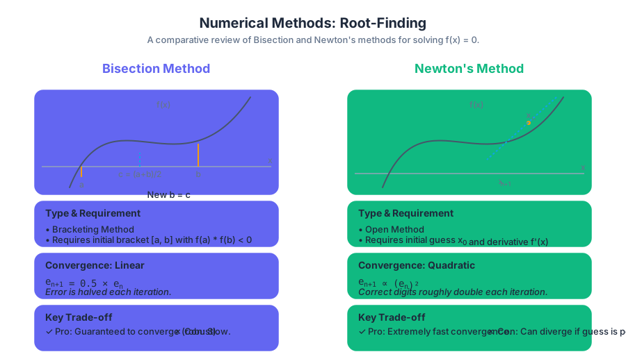
Source Materials
Study CS323: Numerical Analysis and Computing with AI — Free on Lykke
Sign up for free to generate personalized flashcards, quizzes, and study guides from this course. Chat with an AI tutor that knows the material.
Get Started FreeView this course wiki on Lykke · Browse all public course wikis