From the free course CS323: Numerical Analysis and Computing on Lykke
Midterm 2: Review and Assessment
Key concepts: Root-Finding Methods (Newton's, Secant, Bisection) · Convergence Analysis · Polynomial Interpolation (Lagrange, Vandermonde, Newton) · Interpolation Error Analysis · Piecewise vs. Global Interpolation
This module provides a comprehensive review for the second midterm, focusing on root-finding and polynomial interpolation. It includes a practice exam and solutions that test the theoretical understanding and practical application of methods like Newton's, Secant, and various interpolation techniques (Lagrange, Vandermonde, piecewise). Key concepts like convergence rates and error analysis are heavily featured.
Midterm 2: Review and Assessment
This module provides a comprehensive technical review for the second midterm, focusing on the core numerical methods of root-finding and polynomial interpolation. The exam will probe not only your ability to execute these algorithms but also your deeper understanding of their underlying mathematical principles, convergence properties, and the trade-offs that guide their application in real-world scenarios. Mastering these topics requires moving beyond rote memorization to a fluent understanding of why each method behaves as it does.
This guide is structured to mirror the conceptual flow of the course, from finding solutions to single nonlinear equations to approximating complex functions with simpler ones. We will dissect each major algorithm, analyze its performance characteristics, and work through practical examples to solidify your knowledge.
Root-Finding Methods: Seeking f(x) = 0
At its core, root-finding is the process of finding a value x (a root or zero) for which a given function f(x) evaluates to zero. This seemingly simple problem is fundamental across computational science and engineering, appearing in optimization problems (where we find the root of the derivative), equilibrium calculations, and solving systems of nonlinear equations. The midterm will focus on three canonical iterative methods.
The Bisection Method: The Reliable Bracket
-
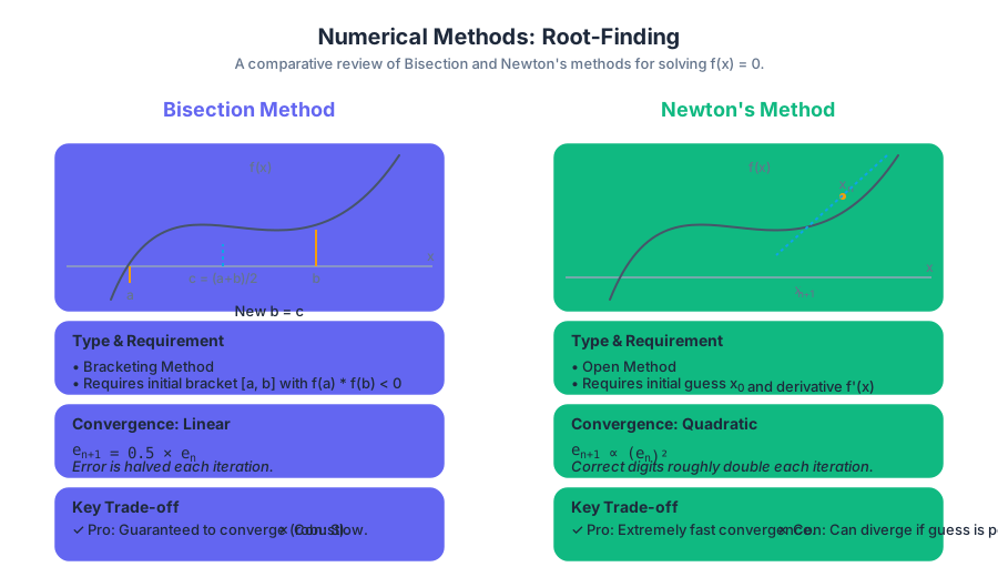
What it is: The Bisection Method is a bracketing method that iteratively narrows down an interval
[a, b]that is known to contain a root. Its operation is guaranteed by the Intermediate Value Theorem, which states that if a continuous functionf(x)has values of opposite sign at the endpoints of an interval (i.e.,f(a) * f(b) < 0), then it must have at least one root within that interval. -
Why it matters: Its primary virtue is its unconditional convergence. As long as the initial bracket is valid, the Bisection Method is guaranteed to find a root. This makes it an incredibly robust and reliable algorithm, often used as a fallback or to generate a safe starting point for faster, but less reliable, methods.
-
How it works:
- Start with an interval
[a, b]such thatf(a)andf(b)have opposite signs. - Calculate the midpoint
c = (a + b) / 2. - Evaluate
f(c). - If
f(c)is sufficiently close to zero,cis the approximate root. - Otherwise, update the bracket:
- If
f(a) * f(c) < 0, the root is in[a, c]. Setb = c. - If
f(b) * f(c) < 0, the root is in[c, b]. Seta = c.
- If
- Repeat from step 2 until the interval
|b - a|is smaller than a specified tolerance.
- Start with an interval
-
Convergence Analysis: The Bisection Method exhibits linear convergence. At each step, the size of the interval containing the root is halved. If
e_nis the error at iterationn(represented by the interval width), thene_{n+1} = 0.5 * e_n. This is a constant factor reduction, which defines linear convergence. While reliable, this is considered slow compared to other methods.
Key Insight: The number of iterations
nrequired to achieve a toleranceεfrom an initial interval[a_0, b_0]can be calculated directly:n ≥ log₂((b_0 - a_0) / ε)This predictability is a unique and powerful feature of the Bisection Method.
- Common Pitfalls:
- Finding a valid initial bracket: For some functions, it can be difficult to find an initial
[a, b]wheref(a)andf(b)have opposite signs. - Multiple roots: If multiple roots exist in the initial bracket, Bisection will find one of them, but it's not predictable which one.
- Performance: Its slow, linear convergence makes it impractical for problems requiring high precision quickly.
- Finding a valid initial bracket: For some functions, it can be difficult to find an initial
Newton's Method: The Tangent Line Approximation
- What it is: Newton's Method (or Newton-Raphson) is an open method that uses tangent lines to iteratively find better approximations to a root. Starting with an initial guess
x_0, it approximates the functionf(x)with its tangent line atx_0and finds where this line intersects the x-axis. This intersection point becomes the next guess,x_1.
The iteration formula is derived from the first-order Taylor expansion of
f(x)aroundx_n:f(x) ≈ f(x_n) + f'(x_n)(x - x_n)Settingf(x) = 0to find the root and solving forx(which becomesx_{n+1}) gives the celebrated formula:x_{n+1} = x_n - f(x_n) / f'(x_n)
-
Why it matters: Speed. When Newton's Method converges, it typically does so extremely fast. This rapid convergence makes it the method of choice for a vast number of applications where efficiency is paramount.
-
How it works:
- Start with an initial guess
x_0that is "reasonably close" to the root. - Calculate the next approximation using the formula
x_{n+1} = x_n - f(x_n) / f'(x_n). - Repeat step 2 until the change
|x_{n+1} - x_n|or the residual|f(x_{n+1})|is below a tolerance.
- Start with an initial guess
Concrete Example: Find the root of f(x) = x² - 2 (i.e., find √2) starting with x_0 = 1.
* f'(x) = 2x
* Iteration 1: x_1 = 1 - (1² - 2) / (2 * 1) = 1 - (-1) / 2 = 1.5
* Iteration 2: x_2 = 1.5 - (1.5² - 2) / (2 * 1.5) = 1.5 - (0.25) / 3 ≈ 1.41667
* Iteration 3: x_3 = 1.41667 - (1.41667² - 2) / (2 * 1.41667) ≈ 1.4142157
The true value of √2 is 1.41421356.... Notice how the number of correct digits roughly doubles with each iteration.
- Convergence Analysis: Newton's Method has quadratic convergence under ideal conditions (the root is simple,
f'(r) ≠ 0, and the initial guess is sufficiently close). This means the errore_{n+1}is proportional to the square of the previous error:e_{n+1} ≈ C * e_n². This is the source of its incredible speed.
import math

def newtons_method(f, df, x0, tol=1e-9, max_iter=100):
    """
    Finds a root of a function using Newton's method.

    Args:
        f (callable): The function for which to find a root, f(x).
        df (callable): The derivative of the function, f'(x).
        x0 (float): Initial guess for the root.
        tol (float): The convergence tolerance.
        max_iter (int): The maximum number of iterations.

    Returns:
        float: The approximate root, or None if the method fails to converge.
    """
    x = x0
    for i in range(max_iter):
        fx = f(x)
        if abs(fx) < tol:
            print(f"Converged after {i} iterations.")
            return x

        dfx = df(x)
        if dfx == 0:
            print("Error: Derivative is zero. Newton's method fails.")
            return None

        x_new = x - fx / dfx

        if abs(x_new - x) < tol:
            print(f"Converged after {i+1} iterations.")
            return x_new

        x = x_new

    print("Warning: Maximum iterations reached. Did not converge.")
    return None

# Example usage: find the root of cos(x) - x^3
f = lambda x: math.cos(x) - x**3
df = lambda x: -math.sin(x) - 3*x**2
root = newtons_method(f, df, x0=0.5)
if root is not None:
    print(f"The root is approximately: {root:.8f}")
    print(f"f(root) = {f(root):.2e}")
# Derivation of Quadratic Convergence for Newton's Method

Let r be the true root, so f(r) = 0. Let e_n = x_n - r be the error at iteration n.
We use a Taylor expansion of f(r) around x_n:
  f(r) = f(x_n) + f'(x_n)(r - x_n) + (f''(ξ_n)/2)(r - x_n)²
  0    = f(x_n) - f'(x_n)e_n + (f''(ξ_n)/2)e_n²

Divide by f'(x_n) (assuming f'(x_n) ≠ 0):
  0 = f(x_n)/f'(x_n) - e_n + (f''(ξ_n)/(2f'(x_n)))e_n²

Rearrange to isolate the term f(x_n)/f'(x_n):
  f(x_n)/f'(x_n) = e_n - (f''(ξ_n)/(2f'(x_n)))e_n²

Now, look at the error in the next step, e_{n+1}:
  e_{n+1} = x_{n+1} - r
          = (x_n - f(x_n)/f'(x_n)) - r
          = (x_n - r) - f(x_n)/f'(x_n)
          = e_n - f(x_n)/f'(x_n)

Substitute the expression for f(x_n)/f'(x_n) from above:
  e_{n+1} = e_n - [e_n - (f''(ξ_n)/(2f'(x_n)))e_n²]
  e_{n+1} = (f''(ξ_n)/(2f'(x_n)))e_n²

As x_n approaches r, ξ_n also approaches r. So for large n:
  e_{n+1} ≈ [f''(r)/(2f'(r))] * e_n²

This shows that e_{n+1} is proportional to e_n², which is the definition of quadratic convergence.
The constant C is f''(r) / (2f'(r)).
- Common Pitfalls:
- Divergence: If the initial guess
x_0is not in the "basin of attraction" for the root, the iterations can diverge to infinity. - Zero Derivative: If
f'(x_n)is zero or very close to it, the next step will be huge or cause a division-by-zero error. This happens at local extrema. - Oscillation: The method can get stuck in a cycle between two or more points without converging.
- Requirement of
f'(x): The analytical derivative must be known and easy to compute, which is not always the case.
- Divergence: If the initial guess
The Secant Method: The Finite-Difference Newton
- What it is: The Secant Method is a clever modification of Newton's Method that avoids the need for an explicit derivative. It approximates the derivative
f'(x_n)using a finite difference based on the two most recent iterates,x_nandx_{n-1}.
The derivative approximation is:
f'(x_n) ≈ (f(x_n) - f(x_{n-1})) / (x_n - x_{n-1})Substituting this into Newton's formula gives the Secant iteration:x_{n+1} = x_n - f(x_n) * (x_n - x_{n-1}) / (f(x_n) - f(x_{n-1}))
-
Why it matters: It provides a practical alternative when the derivative is unavailable or computationally expensive. It almost achieves the speed of Newton's method without its main implementation burden.
-
How it works:
- Start with two initial guesses,
x_0andx_1. - Calculate the next approximation
x_{n+1}using the iteration formula. - Repeat, always using the two most recent points, until convergence is achieved.
- Start with two initial guesses,
-
Convergence Analysis: The Secant Method has superlinear convergence. Its rate is approximately
φ = (1 + √5) / 2 ≈ 1.618(the golden ratio). This meanse_{n+1} ≈ C * e_n^1.618. This is faster than linear but slower than quadratic. In practice, since it only requires one function evaluation per step (compared to two for Newton:fandf'), it can sometimes be faster in terms of wall-clock time. -
Common Pitfalls:
- Requires two initial points.
- It inherits many of the same potential divergence issues as Newton's method, as it is essentially a close approximation.
- If
f(x_n)becomes very close tof(x_{n-1}), the denominator can become small, leading to numerical instability (a form of subtractive cancellation).
Method Comparison
| Feature | Bisection Method | Newton's Method | Secant Method |
|---|---|---|---|
| Convergence Rate | Linear (p=1) |
Quadratic (p=2) |
Superlinear (p≈1.618) |
| Reliability | Guaranteed if bracket is valid | Can diverge | Can diverge |
| Requirements | [a, b] with f(a)f(b)<0 |
f(x), f'(x), and a good x₀ |
f(x) and two initial points x₀, x₁ |
| Cost per Iteration | 1 f evaluation |
1 f eval, 1 f' eval |
1 f evaluation |
| Key Advantage | Robustness & Predictability | Speed | No derivative needed |
| Key Disadvantage | Slow | Needs derivative, can fail | Needs two points, can fail |
Polynomial Interpolation: Connecting the Dots
Polynomial Interpolation is the task of finding a polynomial that passes exactly through a given set of data points. Given n+1 points (x_0, y_0), (x_1, y_1), ..., (x_n, y_n) with distinct x_i, we seek a unique polynomial P_n(x) of degree at most n such that P_n(x_i) = y_i for all i. The choice of basis for representing this polynomial leads to different algorithms with distinct computational trade-offs.
The Vandermonde Approach (Monomial Basis)
- What it is: This is the most direct approach. We assume the polynomial is in the standard monomial basis:
P_n(x) = c_0 + c_1x + c_2x² + ... + c_nx^n. Plugging in each data point(x_i, y_i)creates a system ofn+1linear equations for then+1unknown coefficientsc_j.
This system can be written in matrix form as
Vc = y:[ 1 x₀ x₀² ... x₀ⁿ ] [ c₀ ] [ y₀ ][ 1 x₁ x₁² ... x₁ⁿ ] [ c₁ ] = [ y₁ ][ ... ... ... ... ... ] [ .. ] [ .. ][ 1 xₙ xₙ² ... xₙⁿ ] [ cₙ ] [ yₙ ]The matrixVis the famous Vandermonde matrix.
-
Why it matters: It's a conceptually straightforward way to prove that a unique interpolating polynomial exists (since the Vandermonde matrix is invertible for distinct
x_i). However, it is rarely used in practice due to its severe numerical limitations. -
Pitfalls: The Vandermonde matrix is notoriously ill-conditioned, especially for high degrees and/or clustered points. This means that small errors in the input
y_ican lead to huge errors in the computed coefficientsc_j. Solving the systemVc=yis also computationally expensive, requiringO(n³)operations.
import numpy as np

# Data points to interpolate
x_vals = np.array([0, 1, 3, 4])
y_vals = np.array([2, 1, 5, 3])

# Build the Vandermonde matrix
V = np.vander(x_vals, increasing=True)
print("Vandermonde Matrix V:\n", V)

# Solve the linear system Vc = y for the coefficients c
try:
    coeffs = np.linalg.solve(V, y_vals)
    print("\nCoefficients (c0, c1, c2, c3):", coeffs)

    # Create a polynomial function from the coefficients
    p = np.poly1d(np.flip(coeffs)) # np.poly1d expects coeffs in decreasing power order
    print("\nInterpolating Polynomial P(x):\n", p)

except np.linalg.LinAlgError:
    print("\nCould not solve the system. The Vandermonde matrix may be singular or ill-conditioned.")

# A real-world library call for interpolation often uses a more stable basis internally.
# For example, using SciPy's BarycentricInterpolator which is related to Lagrange.
from scipy.interpolate import BarycentricInterpolator

poly_bary = BarycentricInterpolator(x_vals, y_vals)
print(f"\nValue at x=2 (using a stable library method): {poly_bary(2.0)}")
The Lagrange Basis
- What it is: The Lagrange approach constructs the polynomial differently. Instead of solving for coefficients, it builds the final polynomial as a weighted sum of special Lagrange basis polynomials,
L_j(x).
The interpolating polynomial is
P_n(x) = Σ_{j=0}^{n} y_j * L_j(x), where eachL_j(x)is a polynomial of degreenwith the property thatL_j(x_i) = 1ifi=jand0ifi≠j.L_j(x) = Π_{i=0, i≠j}^{n} (x - x_i) / (x_j - x_i)
-
Why it matters: It provides an elegant, explicit formula for the interpolating polynomial without needing to solve a linear system. The "coefficients" are simply the
y_ivalues themselves. -
Pitfalls:
- Evaluation is expensive: Evaluating
P_n(x)at a new point takesO(n²)operations. - Not adaptive: If a new data point
(x_{n+1}, y_{n+1})is added, all the basis polynomialsL_j(x)must be recomputed from scratch. This makes it inflexible.
- Evaluation is expensive: Evaluating
The Newton Basis
-
What it is: The Newton form represents the polynomial in a basis that is built up incrementally. This is arguably the most practical and computationally sound approach.
P_n(x) = c_0 + c_1(x-x_0) + c_2(x-x_0)(x-x_1) + ... + c_n(x-x_0)...(x-x_{n-1}) -
Why it matters: It strikes an excellent balance between computational efficiency and flexibility.
- Efficient Coefficient Calculation: The coefficients
c_j(called divided differences) can be computed inO(n²)time using a dynamic programming approach. - Efficient Evaluation: The nested structure of the Newton form can be evaluated in
O(n)time using Horner's method. - Adaptive: Adding a new data point only requires computing one new row in the divided differences table; all previous coefficients remain unchanged.
- Efficient Coefficient Calculation: The coefficients
-
How it works: The coefficients
c_jare the diagonal entries of a divided differences table.c_0 = f[x_0] = y_0c_1 = f[x_0, x_1] = (y_1 - y_0) / (x_1 - x_0)c_2 = f[x_0, x_1, x_2] = (f[x_1, x_2] - f[x_0, x_1]) / (x_2 - x_0)- ...and so on.
function build_divided_diff_table(x_points, y_points):
    n = length(x_points)
    // Initialize a 2D array (table) of size n x n
    table = new array[n][n]

    // The first column is just the y-values
    for i from 0 to n-1:
        table[i][0] = y_points[i]

    // Fill the rest of the table
    for j from 1 to n-1: // Column index
        for i from j to n-1: // Row index
            numerator = table[i][j-1] - table[i-1][j-1]
            denominator = x_points[i] - x_points[i-j]
            table[i][j] = numerator / denominator

    // The coefficients are the top diagonal: table[0][0], table[1][1], ...
    coefficients = []
    for i from 0 to n-1:
        coefficients.append(table[i][i])

    return coefficients
Basis Comparison
| Feature | Monomial (Vandermonde) | Lagrange | Newton |
|---|---|---|---|
| Coefficient Cost | O(n³) (solve system) |
O(1) (they are the yᵢ) |
O(n²) (build table) |
| Evaluation Cost | O(n) (Horner's method) |
O(n²) |
O(n) (nested form) |
| Adding a New Point | O(n³) (re-solve) |
O(n²) (re-build all Lⱼ) |
O(n) (add one row to table) |
| Numerical Stability | Very Poor (ill-conditioned) | Moderate | Good |
| Primary Use Case | Theoretical proofs | Mathematical elegance | Practical implementation |
Error Analysis and Advanced Topics
A common exam theme is understanding when and why interpolation fails. Simply increasing the degree of the polynomial is not a panacea for achieving better accuracy.
The Interpolation Error Formula
If
f(x)is a sufficiently smooth function andP_n(x)is the polynomial that interpolatesfatn+1distinct pointsx_0, ..., x_n, then for anyxin the interval containing the nodes, the errorE(x) = f(x) - P_n(x)is given by:E(x) = (f^(n+1)(ξ) / (n+1)!) * Π_{i=0}^{n} (x - x_i)for someξin the interval.
This formula is crucial. It tells us that the error depends on two things:
- The function itself: via the
(n+1)-th derivative. If the function is "wiggly" (has large derivatives), the error will be large. - The choice of interpolation points: via the nodal polynomial
ω(x) = Π(x - x_i). The error is zero at the nodes and largest between them.
Runge's Phenomenon: The Peril of High-Degree Interpolation
-
What it is: Runge's Phenomenon is the classic example of the failure of high-degree global interpolation. When interpolating the function
f(x) = 1 / (1 + 25x²)on the interval[-1, 1]with a high-degree polynomial using equally spaced nodes, the polynomial exhibits wild oscillations near the endpoints, causing the error to grow, not shrink, as more points are added. -
Why it happens: For the Runge function, the high-order derivatives
f^(n+1)(x)grow very rapidly, especially near the endpoints. At the same time, for equally spaced points, the nodal polynomialω(x)is largest near the endpoints. The product of these two large terms in the error formula leads to catastrophic error.
# Using gnuplot to visualize Runge's Phenomenon

# Set up the plot environment
gnuplot -persist <<-EOF
    set title "Runge's Phenomenon: Interpolating f(x) = 1/(1+25x^2)"
    set xlabel "x"
    set ylabel "y"
    set grid
    set key top center
    set samples 500
    set xrange [-1:1]
    set yrange [-1:2]

    # Define the Runge function
    f(x) = 1.0 / (1.0 + 25.0 * x**2)

    # Plot the original function and data points for N=11
    # Gnuplot can't do polynomial interpolation directly, so we generate data points
    # that would be used by an external script. This script visualizes the concept.
    plot f(x) with lines lw 2 title "Original f(x)", \
         '<(for i in {-5..5}; do x=$(echo "$i/5.0" | bc -l); y=$(echo "1/(1+25*$x*$x)" | bc -l); echo "$x $y"; done)' \
         with points pt 7 ps 1.5 title "11 Equally Spaced Nodes"
EOF

# In a real analysis, one would pipe these points to a Python script
# to compute the 10th-degree interpolant and plot it back.
# The command demonstrates how to generate the nodes for visualization.
# The resulting plot would show a polynomial that matches the points but
# wildly oscillates between them, especially near x=-1 and x=1.
Piecewise vs. Global Interpolation
-
The Solution: To avoid Runge's phenomenon and the instability of high-degree polynomials, the universal modern approach is piecewise interpolation. Instead of using one polynomial of degree
nforn+1points, we break the domain into subintervals and use a separate low-degree polynomial (e.g., linear, cubic) on each piece. -
Piecewise Linear Interpolation: Simply connect adjacent data points with straight lines. This is simple and robust but not smooth (the derivative is discontinuous at the nodes).
-
Splines: Splines are more sophisticated piecewise polynomials (most commonly, cubic splines) that are constrained to have continuous derivatives at the nodes. This results in a curve that is both accurate locally and smooth globally. They are the foundation of modern computer graphics, CAD software, and data visualization.
| Feature | Global Polynomial Interpolation | Piecewise Interpolation (e.g., Splines) |
|---|---|---|
| Polynomial Degree | High (n) | Low (e.g., 1 or 3) |
| Smoothness | Infinitely differentiable | Controllable (e.g., C² for cubic splines) |
| Runge's Phenomenon | Highly susceptible | Immune |
| Local Control | No (changing one point affects the entire curve) | Yes (changing one point only affects nearby segments) |
| Computational Cost | High (O(n³) or O(n²)) |
Low (often linear in n) |
| Typical Use | Function approximation over small, well-behaved domains | Standard for data fitting, graphics, engineering |
Source Materials
Study CS323: Numerical Analysis and Computing on Lykke
This course page is free to open: signed out, you can read its first two sections, and signing in, on any plan, opens the rest. The free Lykke Chrome extension syncs your own Canvas courses, so ChatGPT, Claude and Muse can answer from your classes and deadlines. It only reads Canvas.
Add the free extensionSign in to open every sectionAll sections of CS323: Numerical Analysis and Computing · Browse more course pages