Computing
Institution: MIT
42 study materials · 11 sections
The Client Challenge course is a comprehensive introduction to computer science and programming using the Python language, specifically designed for beginners. It guides students through the fundamentals of computational thinking, starting with basic variables and arithmetic expressions before moving into complex logic and simulations. By the end of the course, learners will be able to design modular programs, handle data structures like lists and strings, and understand the ethical implications of algorithmic bias.
Course Sections
Introduction to Computational Thinking
Key concepts: Computational thinking · Sequence and state · Program execution
An introduction to how computers interpret instructions and the foundational concept of computational thinking.
Introduction to Computational Thinking
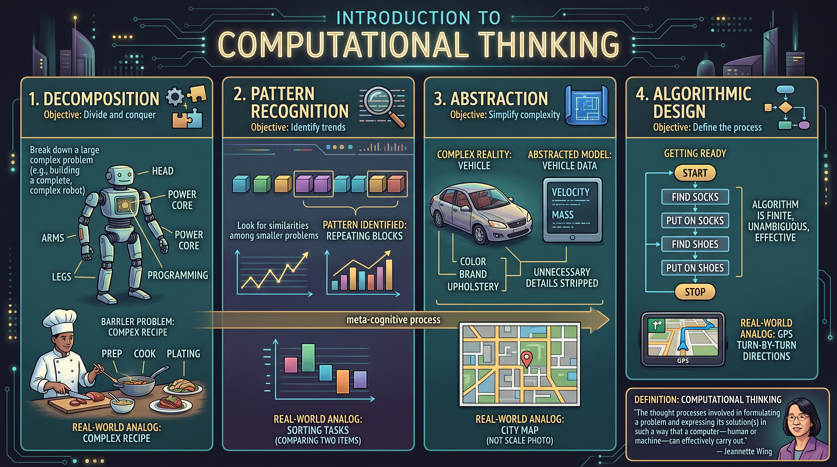
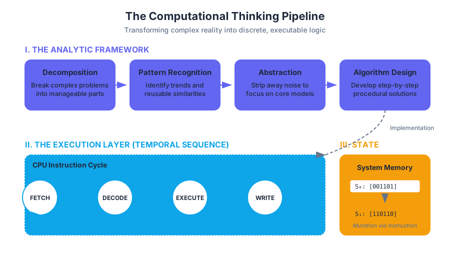
Computational thinking is not merely the act of writing code; it is a fundamental analytic skill that involves solving problems, designing systems, and understanding human behavior by drawing on the concepts fundamental to computer science. While a programmer uses a language to communicate with a machine, a computational thinker uses a framework to decompose reality into discrete, executable logic.
The Pillars of Computational Thinking
At its core, computational thinking is a meta-cognitive process. It allows us to take a complex, often ambiguous problem and reformulate it into a format that a procedural agent—be it a human following a recipe or a CPU executing binary—can resolve with precision.
1. Decomposition
Decomposition is the practice of breaking a complex problem down into smaller, more manageable parts. In software engineering, this is often referred to as modularity. By isolating components, we reduce the cognitive load required to solve any single piece of the puzzle.
2. Pattern Recognition
Once a problem is decomposed, we look for similarities among the smaller problems. Recognizing these patterns allows us to apply previously discovered solutions to new contexts, leading to efficiency and the creation of reusable logic.
3. Abstraction
Abstraction involves stripping away the unnecessary details to focus on the general mechanisms that matter. It is the process of creating a "model" of the problem. For instance, when modeling a vehicle in a simulation, we might care about its velocity and mass, but ignore its color or the brand of its upholstery.
4. Algorithmic Design
This is the culmination of the previous three steps: developing a step-by-step strategy for solving the problem. An algorithm must be finite, unambiguous, and effective.
| Pillar | Objective | Real-World Analog |
|---|---|---|
| Decomposition | Divide and conquer | Breaking a large recipe into prep, cooking, and plating. |
| Pattern Recognition | Identify trends | Noticing that all "sorting" tasks involve comparing two items. |
| Abstraction | Simplify complexity | Using a map instead of a 1:1 scale photograph of a city. |
| Algorithm Design | Define the process | Writing the turn-by-turn directions for a GPS. |
Definition: Computational Thinking "The thought processes involved in formulating a problem and expressing its solution(s) in such a way that a computer—human or machine—can effectively carry out." — Jeannette Wing
Sequence and the Temporal Nature of Execution
In computing, the sequence refers to the specific, linear order in which instructions are processed. Because computers are deterministic, the order of operations is the primary determinant of the final outcome. A single transposed line of code can be the difference between a successful transaction and a system crash.
The Fetch-Decode-Execute Cycle
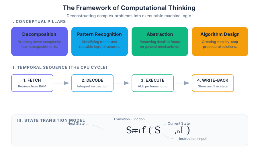
To understand sequence, one must understand how the hardware processes it. Every instruction follows a rigid lifecycle within the Central Processing Unit (CPU):
- Fetch: The instruction is retrieved from memory (RAM) based on the current value of the Program Counter.
- Decode: The Control Unit interprets the binary instruction to determine what operation is required.
- Execute: The Arithmetic Logic Unit (ALU) performs the operation.
- Write-back: The result is stored back into memory or a register.
Determinism and Linearity
Unless directed otherwise by control flow structures (like loops or conditionals), a program executes from the top down. This linearity ensures that the state of the system at line $n$ is a direct result of all operations from lines $1$ to $n-1$.
Worked Example: The Importance of Sequence
Consider a simple banking operation. If we reverse the sequence of "Check Balance" and "Withdraw Funds," we risk an overdraft because the state was not validated before the mutation occurred.
| Step | Correct Sequence | Incorrect Sequence | Result of Error |
|---|---|---|---|
| 1 | Check if balance > $100 | Deduct $100 | Negative balance allowed |
| 2 | Deduct $100 | Check if balance > $100 | Logic check happens too late |
| 3 | Update Database | Update Database | Integrity compromised |
State: The Memory of the Machine
If sequence is the "verb" of computation, state is the "noun." State represents the condition of a system at a specific point in time, stored in the computer's memory as variables, data structures, or register values.
Variables as State Containers
A variable is a symbolic name for a memory location. When we assign a value to a variable, we are modifying the state of the program.
State Transitions
A program is essentially a State Machine. It moves from an initial state $S_0$ through a series of transitions $T$ triggered by instructions, eventually reaching a final state $S_{final}$.
$$S_{n+1} = f(S_n, I)$$
Where $S$ is the state and $I$ is the instruction. This mathematical representation highlights that the next state is strictly a function of the current state and the current instruction.
Implementation: Low-Level State Management
In systems programming, managing state often requires direct interaction with memory addresses. The following C example demonstrates how state is modified by manipulating memory directly.
#include <stdio.h>

/**
 * Demonstrates state transition through pointer manipulation.
 * In low-level systems, 'state' is literally the bits stored
 * at a specific hex address in RAM.
 */
int main() {
    // Initial State: memory is allocated for an integer
    int system_state = 100;
    int *state_ptr = &system_state;

    printf("Initial State Value: %d at Address: %p\n", system_state, (void*)state_ptr);

    // Transition: Instruction modifies the value at the address
    *state_ptr = 250;

    // Final State: The value at the memory location has changed
    if (system_state == 250) {
        printf("State Transition Successful. New Value: %d\n", system_state);
    }

    return 0;
}
Program Execution and Tracing
Program execution is the process by which a computer interprets the source code and transforms it into actions. This can happen via Compilation (translating the whole program to machine code at once) or Interpretation (translating and executing line-by-line).
Tracing Logic
Tracing is a mental or manual technique used by programmers to track the value of variables as they change through a sequence. It is the most effective way to debug logic errors.
Formal Representation of Execution
We can represent the execution of a simple algorithm using a Trace Table. This allows us to visualize the "movement" of state through the sequence.
ALGORITHM: SumFirstN
1. INPUT n
2. SET total = 0
3. SET counter = 1
4. WHILE counter <= n:
5.    total = total + counter
6.    counter = counter + 1
7. OUTPUT total

TRACE TABLE (Input n = 3):
| Line | n | total | counter | counter <= n |
|------|---|-------|---------|--------------|
| 1    | 3 | ?     | ?       | ?            |
| 2    | 3 | 0     | ?       | ?            |
| 3    | 3 | 0     | 1       | ?            |
| 4    | 3 | 0     | 1       | True         |
| 5    | 3 | 1     | 1       | True         |
| 6    | 3 | 1     | 2       | True         |
| 4    | 3 | 1     | 2       | True         |
| 5    | 3 | 3     | 2       | True         |
| 6    | 3 | 3     | 3       | True         |
| 4    | 3 | 3     | 3       | True         |
| 5    | 3 | 6     | 3       | True         |
| 6    | 3 | 6     | 4       | True         |
| 4    | 3 | 6     | 4       | False        |
| 7    | 3 | 6     | 4       | -            |
Data Types and Arithmetic Expressions
Computational thinking requires us to categorize data. Computers do not "know" what a number or a letter is; they only know bits. Data Types provide the context the computer needs to interpret those bits correctly.
Primitive Data Types
Most languages support a core set of primitives:
- Integers: Whole numbers (e.g.,
42,-7). - Floats/Doubles: Decimal numbers (e.g.,
3.14159). - Booleans: Truth values (
True,False). - Strings: Sequences of characters (
"Hello World").
Operator Precedence
When executing arithmetic expressions, computers follow a strict hierarchy known as Order of Operations (often PEMDAS/BODMAS). In computational thinking, we must be explicit about this to avoid "off-by-one" errors or precision loss.
| Operator Category | Symbols | Precedence Level |
|---|---|---|
| Parentheses | () |
1 (Highest) |
| Exponentiation | ** or ^ |
2 |
| Multiplication/Division | *, /, //, % |
3 |
| Addition/Subtraction | +, - |
4 (Lowest) |
Real-World Usage: Data Normalization
In a real-world scenario, such as a data pipeline, we use computational thinking to transform raw input into a standardized format.
import math

def process_sensor_data(raw_value, scale_factor, offset):
    """
    Example of an arithmetic expression in a real-world pipeline.
    Applies a linear transformation and rounds to significant digits.
    """
    # Computational Step: Normalize the input
    # Formula: (value * scale) + offset
    normalized = (raw_value * scale_factor) + offset

    # Abstraction: We only care about 2 decimal places for this state
    final_state = round(normalized, 2)

    return final_state

# Usage in a simulated environment
current_temp_raw = 1024
celsius = process_sensor_data(current_temp_raw, 0.03125, -20.0)
print(f"Processed State: {celsius}°C")
Common Pitfalls in Computational Thinking
Even experienced engineers fall into traps when translating human logic into machine execution.
1. Logic Errors vs. Syntax Errors
A Syntax Error is a "grammar" mistake in the code that prevents it from running. A Logic Error is a flaw in the computational thinking process itself—the code runs, but it produces the wrong result. Logic errors are far more dangerous because they do not trigger immediate failures.
2. The "Off-By-One" Error
This occurs frequently in sequence design, particularly when dealing with loops or list indexing. It happens when a programmer fails to account for whether a sequence is zero-indexed or one-indexed.
3. Floating Point Imprecision
Computers represent decimals in binary, which cannot perfectly represent certain fractions (like 0.1).
- Pitfall: Comparing two floats for equality (
if x == 0.3). - Solution: Use a small "epsilon" range for comparisons (
if abs(x - 0.3) < 0.00001).
4. State Side Effects
Modifying a global state from within a local sequence can lead to unpredictable behavior. This is why modern computational thinking emphasizes immutability and pure functions where possible.
| Error Type | Cause | Detection Method |
|---|---|---|
| Syntax | Incorrect language usage | Compiler/Interpreter feedback |
| Runtime | Illegal operations (e.g., Divide by Zero) | Crash reports / Exceptions |
| Logic | Flawed algorithm design | Unit testing / Manual tracing |
| Semantic | Meaningless but valid code | Peer review / Static analysis |
Debugging: The Scientific Method of Code
Debugging is the application of the scientific method to computational thinking. When a program fails, we:
- Observe the incorrect behavior.
- Hypothesize which part of the sequence or state is flawed.
- Experiment by modifying the code.
- Analyze the results to see if the state now matches expectations.
The Rubber Duck Technique
A famous debugging method involves explaining your code, line-by-line, to an inanimate object (like a rubber duck). This forces the brain to switch from "skimming" to "executing" the logic, often revealing gaps in the sequence that were previously overlooked.
Summary of Execution Flow
To master computational thinking, one must visualize the program not as a static document, but as a dynamic flow of data.
- Input: Data enters the system (Initial State).
- Process: The sequence of instructions manipulates the data.
- Storage: Intermediate states are saved in variables.
- Output: The final state is presented to the user or another system.
This cycle is the heartbeat of every piece of software, from the simplest script to the most complex artificial intelligence. By mastering the relationship between sequence and state, you gain the ability to build robust, scalable, and efficient solutions to any problem.
Variables and Data Types
Key concepts: Variables · Data types · Arithmetic expressions
Learning how to store and manipulate information using variables and basic data types in Python.
Variables and Data Types: The Foundations of Computational State
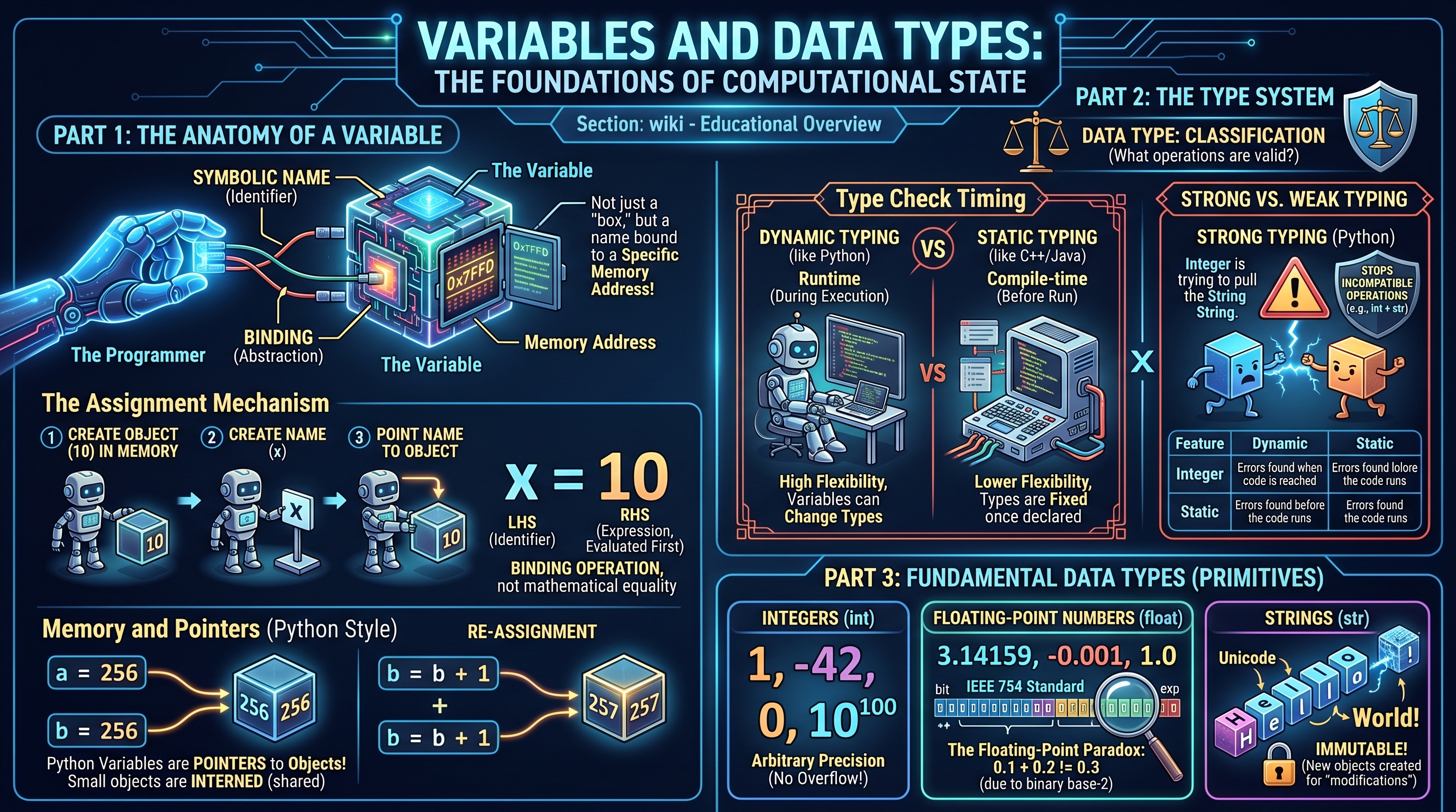
In the realm of computer science, we transition from being mere consumers of software to being architects of logic. At the heart of this transition lies the ability to represent, store, and manipulate information. This is achieved through Variables and Data Types. To the uninitiated, a variable is a "box" that holds a value. To the engineer, a variable is a symbolic name—an abstraction—bound to a specific memory address, governed by a type system that dictates how many bits that value occupies and what operations are valid upon it.
The Anatomy of a Variable
A variable is a fundamental unit of storage in a program. It allows a programmer to refer to a value by a name rather than by its physical location in the computer's Random Access Memory (RAM). This process of naming is known as identifier binding.
The Assignment Mechanism
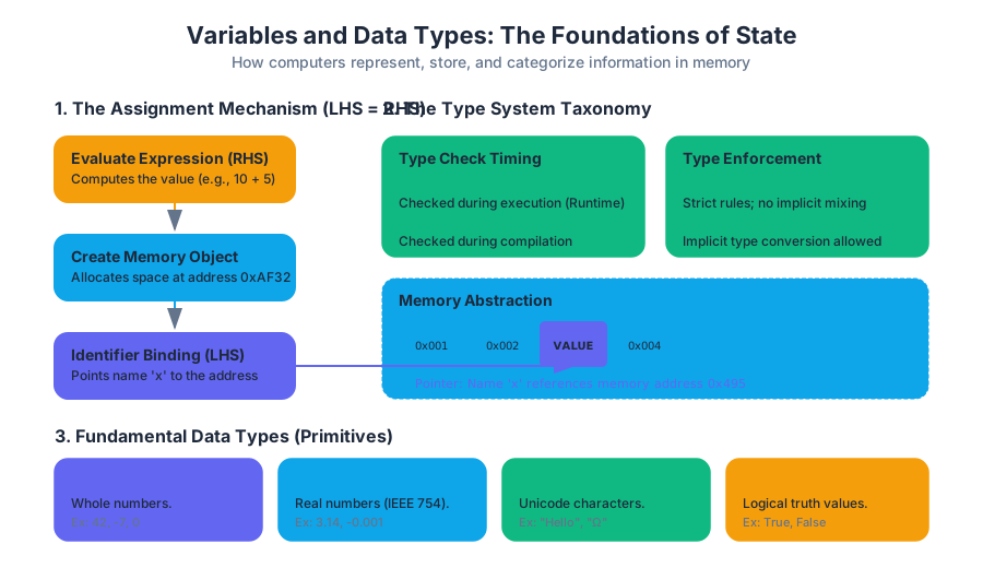
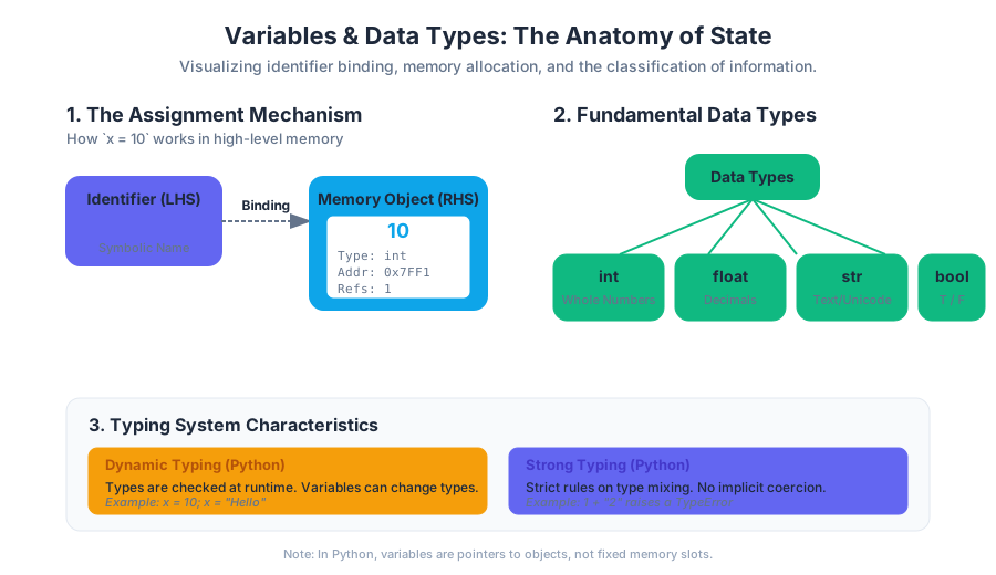
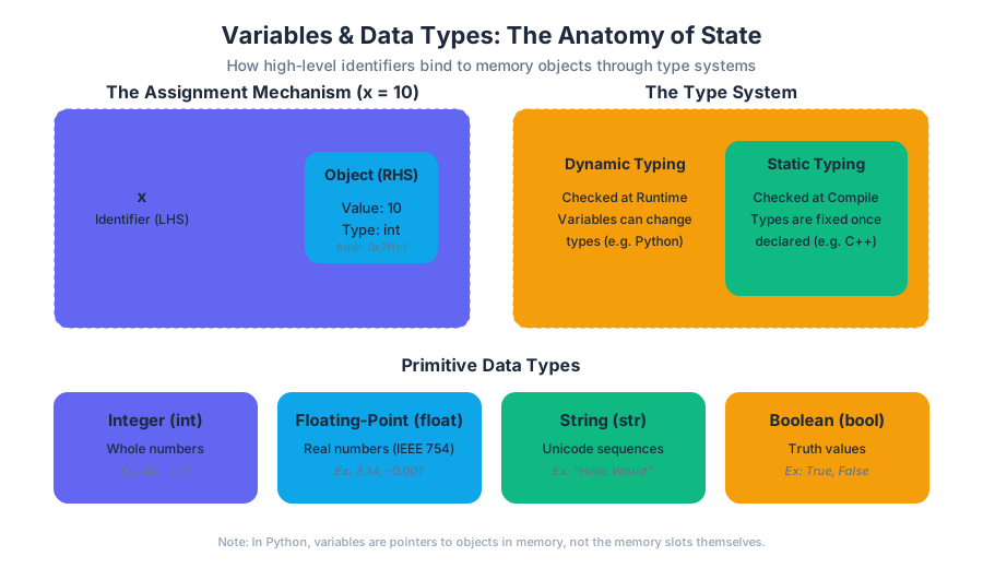
In Python and many other high-level languages, the assignment operator = does not represent mathematical equality. Instead, it represents a binding operation. When we write x = 10, we are instructing the interpreter to:
- Create an object in memory to represent the integer
10. - Create the name
x(if it doesn't already exist). - Point the name
xto the memory address of the object10.
Definition: The Assignment Statement An assignment statement evaluates the expression on the right-hand side (RHS) first, and then associates the resulting value with the identifier on the left-hand side (LHS).
Memory and Pointers
Unlike low-level languages like C, where a variable is a specific "slot" in memory, Python variables are pointers to objects. This distinction is crucial for understanding how data is shared and modified within a system.
# Block 1: Low-level implementation/Object Identity in Python
# Demonstrating how variables point to memory addresses (IDs)

def investigate_memory():
    # Integer assignment
    a = 256
    b = 256

    # In Python, small integers are cached (interned)
    print(f"Value a: {a}, Address: {hex(id(a))}")
    print(f"Value b: {b}, Address: {hex(id(b))}")
    print(f"Are they the same object? {a is b}")

    # Re-assignment: b now points to a new object
    b = b + 1
    print(f"New Value b: {b}, New Address: {hex(id(b))}")

    # List mutation vs Re-assignment
    list_a = [1, 2, 3]
    list_b = list_a # Both names point to the same memory block
    list_a.append(4)
    print(f"list_b after list_a mutation: {list_b}") # list_b changes because it shares the object

investigate_memory()
The Type System: Categorizing Information
A Data Type is a classification of data which tells the compiler or interpreter how the programmer intends to use the data. It defines the set of values the data can take and the operations that can be performed on it.
Static vs. Dynamic Typing
Python is dynamically typed, meaning the type of a variable is determined at runtime based on the value it currently holds. This contrasts with statically typed languages (like Java or C++), where the type must be declared explicitly before the program runs.
Strong vs. Weak Typing
Python is also strongly typed. This means the language prevents operations on incompatible types (e.g., you cannot add a string to an integer without explicit conversion).
| Feature | Dynamic Typing (Python) | Static Typing (C++/Java) |
|---|---|---|
| Type Check Timing | During execution (Runtime) | During compilation (Compile-time) |
| Flexibility | High; variables can change types | Low; types are fixed once declared |
| Performance | Slower (overhead of checking types) | Faster (types are pre-determined) |
| Error Detection | Errors found when code is reached | Errors found before the code runs |
Fundamental Data Types
In computational thinking, we categorize data into "primitives." These are the building blocks for all complex data structures.
1. Integers (int)
Integers represent whole numbers (positive, negative, or zero). In modern Python (version 3+), integers have arbitrary precision, meaning they can grow as large as the available memory allows, avoiding the "overflow" errors common in older languages.
2. Floating-Point Numbers (float)
Floats represent real numbers with fractional parts. They are implemented using the IEEE 754 standard for double-precision binary floating-point arithmetic.
The Floating-Point Paradox: Because computers use binary (base-2) to represent decimals, some base-10 fractions (like 0.1) cannot be represented exactly. This leads to precision errors, such as
0.1 + 0.2resulting in0.30000000000000004.
3. Strings (str)
Strings are sequences of Unicode characters. They are immutable, meaning once a string is created, it cannot be changed in place. Any "modification" to a string actually creates a new string object in memory.
4. Booleans (bool)
Representing truth values: True or False. These are essential for control flow and decision-making logic.
/* Block 2: Low-level C representation of Data Types */
/* This shows how different types occupy specific byte-widths in memory */

#include <stdio.h>

int main() {
    int integerVar = 42;           // Typically 4 bytes
    float floatVar = 3.14f;        // Typically 4 bytes (IEEE 754)
    double doubleVar = 3.14159;    // Typically 8 bytes
    char charVar = 'A';            // 1 byte (ASCII)

    printf("Size of int: %zu bytes\n", sizeof(integerVar));
    printf("Size of float: %zu bytes\n", sizeof(floatVar));
    printf("Size of char: %zu bytes\n", sizeof(charVar));

    // Binary representation of the integer 42:
    // 00000000 00000000 00000000 00101010
    return 0;
}
Arithmetic Expressions and Operator Precedence
Computers excel at evaluating arithmetic expressions. An expression is a combination of values, variables, and operators that the Python interpreter evaluates to produce a single value.
The Hierarchy of Operations
To resolve complex calculations, Python follows a strict order of operations, often remembered by the acronym PEMDAS (Parentheses, Exponents, Multiplication/Division, Addition/Subtraction).
| Operator | Name | Description | Example |
|---|---|---|---|
** |
Exponentiation | Raises the LHS to the power of the RHS | 2 ** 3 = 8 |
% |
Modulo | Returns the remainder of division | 10 % 3 = 1 |
// |
Floor Division | Divides and rounds down to the nearest whole number | 10 // 3 = 3 |
/ |
Division | Standard division (always returns a float) | 10 / 2 = 5.0 |
* |
Multiplication | Standard multiplication | 4 * 5 = 20 |
+ |
Addition | Sums two values | 5 + 2 = 7 |
- |
Subtraction | Subtracts the RHS from the LHS | 5 - 2 = 3 |
The Modulo Operator in Practice
The modulo operator (%) is frequently used in algorithms to:
- Check for parity:
n % 2 == 0is true ifnis even. - Keep values within a range: Useful for cyclic patterns, such as clock arithmetic or wrapping a player around a screen in a game.
Program Execution and State Tracing
Understanding how a program moves through lines of code is known as Program Execution. Computers execute code sequentially, from top to bottom, unless directed otherwise by control structures.
State Tracing
The "state" of a program is the current value of all variables at a specific point in time. Tracing is the manual or automated process of tracking these values to debug logic errors.
Example Trace Table: Consider the following code:
x = 10
y = 5
x = x + y
y = x - y
x = x - y
| Line # | Variable x |
Variable y |
Notes |
|---|---|---|---|
| 1 | 10 | undefined | x initialized |
| 2 | 10 | 5 | y initialized |
| 3 | 15 | 5 | x becomes 15 |
| 4 | 15 | 10 | y becomes 10 (15 - 5) |
| 5 | 5 | 10 | x becomes 5 (15 - 10) |
Insight: This specific sequence of operations is a classic algorithm for swapping two variables without using a temporary third variable.
User Input and Type Casting
Programs become interactive when they accept User Input. In Python, the input() function pauses execution and waits for the user to type something.
Crucial Rule: The
input()function always returns data as a String, regardless of what the user types.
Type Casting (Conversion)
To perform calculations on user input, we must "cast" the data into the appropriate type. This is the process of converting a value from one data type to another.
| Function | Target Type | Use Case | Example |
|---|---|---|---|
int() |
Integer | Converting numeric strings to whole numbers | int("42") |
float() |
Float | Converting numeric strings to decimals | float("3.14") |
str() |
String | Converting numbers to text for concatenation | str(100) |
bool() |
Boolean | Evaluating the "truthiness" of a value | bool(1) (True) |
# Block 3: Real-world Usage Example
# A script to calculate Body Mass Index (BMI) demonstrating input, casting, and expressions

def calculate_bmi():
    print("--- Health Metrics Calculator ---")

    try:
        # Input returns strings, so we must cast to float for math
        weight_kg = float(input("Enter your weight in kg: "))
        height_m = float(input("Enter your height in meters: "))

        # BMI Formula: weight / (height^2)
        bmi = weight_kg / (height_m ** 2)

        # Using f-strings (formatted strings) for output
        print(f"Your calculated BMI is: {bmi:.2f}")

        if bmi < 18.5:
            print("Status: Underweight")
        elif 18.5 <= bmi < 25:
            print("Status: Normal weight")
        else:
            print("Status: Overweight")

    except ValueError:
        print("Error: Please enter valid numeric values.")

# calculate_bmi()
Debugging: Syntax, Runtime, and Logic Errors
As a professor of computer science, I often tell my students: "Programming is 10% writing code and 90% debugging it." Understanding the types of errors that occur with variables and data types is essential.
1. Syntax Errors
These occur when the code violates the rules of the language (the "grammar"). The computer cannot even begin to run the program.
- Example:
x = 10 +(Missing an operand).
2. Runtime Errors (Exceptions)
The code is syntactically correct, but an error occurs during execution.
- Example:
y = 10 / 0(ZeroDivisionError) orint("hello")(ValueError).
3. Logic Errors
The program runs without crashing, but it produces the wrong output. These are the hardest to find.
- Example: Using
x + ywhen you meantx * y.
Advanced Concept: Immutability and Memory Optimization
In Python, certain types are immutable (Integers, Floats, Strings, Booleans, Tuples). When you "change" an immutable variable, you aren't changing the data in place; you are creating a new object and moving the pointer.
Why Immutability Matters
- Thread Safety: Immutable objects can be shared across different parts of a program without risk of one part changing the value unexpectedly.
- Hashability: Only immutable objects can be used as keys in a dictionary (a concept we will explore in later modules).
- Performance: Python optimizes memory by "interning" small integers and certain strings, meaning multiple variables pointing to the value
100actually point to the exact same memory address.
Debugging Strategies
Key concepts: Syntax errors · Runtime errors · Logic errors · Program tracing
Identifying and fixing different types of errors that occur during the programming process.
Debugging Strategies
In the realm of computer science, the act of programming is rarely a linear path from conception to execution. Rather, it is a cyclical process of hypothesis, implementation, and refinement. Debugging is the systematic process of identifying, isolating, and fixing "bugs"—defects or problems in a computer program that prevent it from operating correctly. To the novice, debugging is a frustration; to the expert, it is a forensic science.
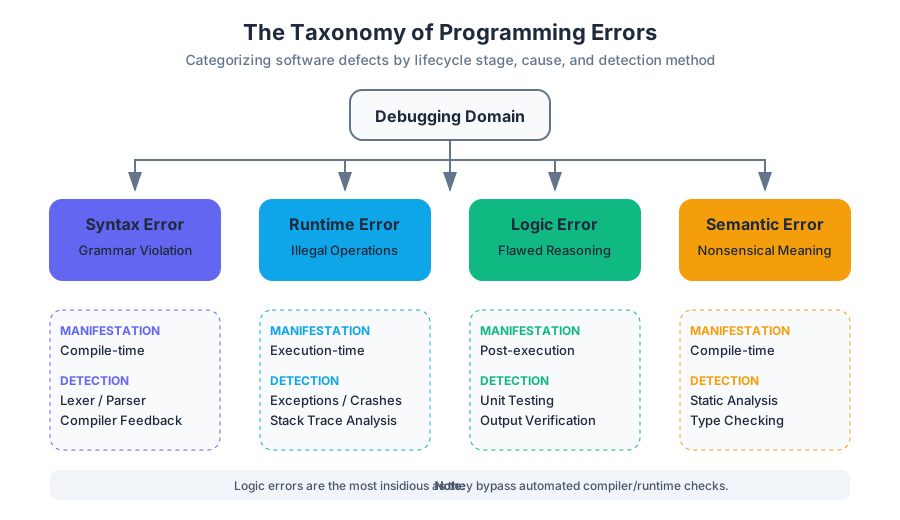
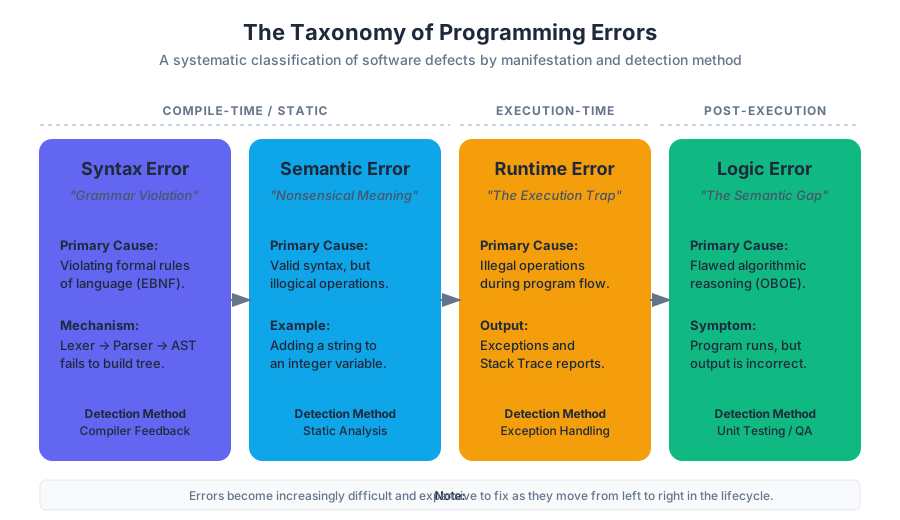
The Taxonomy of Errors
Before one can master the strategies of resolution, one must understand the anatomy of the failure. Errors are generally categorized by the stage of the development lifecycle in which they manifest.
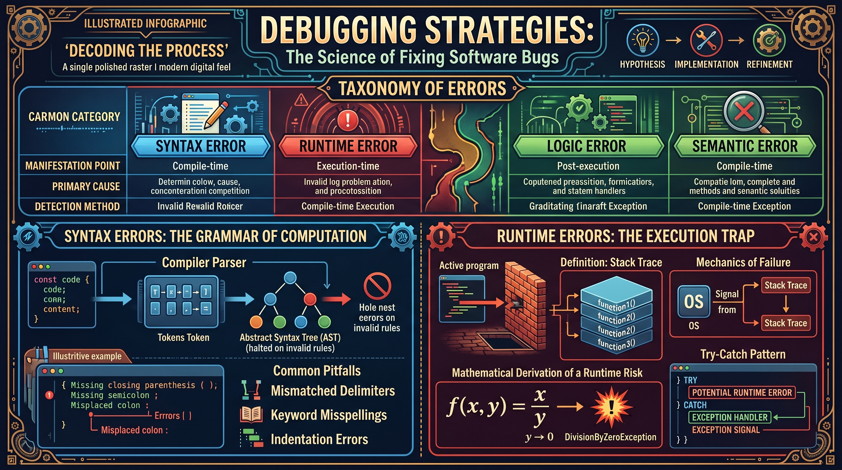
| Error Category | Manifestation Point | Primary Cause | Detection Method |
|---|---|---|---|
| Syntax Error | Compile-time / Interpretation-time | Violation of language grammar | Parser/Compiler feedback |
| Runtime Error | Execution-time | Illegal operations (e.g., Div by Zero) | Exception handling / Crashes |
| Logic Error | Post-execution | Flawed algorithmic reasoning | Unit testing / Output verification |
| Semantic Error | Compile-time | Valid syntax, but nonsensical meaning | Static analysis |
Syntax Errors: The Grammar of Computation
A Syntax Error occurs when the code violates the structural rules of the programming language. Just as a natural language has rules for sentence structure, programming languages have strict formal grammars, often defined by Extended Backus-Naur Form (EBNF).
What it is
The compiler or interpreter acts as a linguist. When it encounters a sequence of tokens that does not match any valid production rule in the language's grammar, it halts execution. Because the computer cannot "guess" the programmer's intent, even a single missing character can render a million-line system unrunnable.
How it works
Modern compilers use a Lexer to turn characters into tokens (keywords, identifiers, operators) and a Parser to build an Abstract Syntax Tree (AST). A syntax error occurs when the Parser reaches a state where no valid transition exists for the next token.
/*
   Example 1: Low-level C implementation demonstrating
   common syntax errors in a memory allocation routine.
*/

#include <stdio.h>
#include <stdlib.h>

int main() {
    int *arr;
    int size = 10;

    // SYNTAX ERROR: Missing closing parenthesis in malloc call
    // SYNTAX ERROR: Missing semicolon at the end of the line
    arr = (int *)malloc(size * sizeof(int)

    if (arr == NULL) {
        printf("Allocation failed\n");
        return 1;
    }

    for (int i = 0; i < size; i++) {
        // SYNTAX ERROR: Using a colon instead of a semicolon in loop
        arr[i] = i * 2:
    }

    free(arr);
    return 0;
}
Common Pitfalls
- Mismatched Delimiters: Forgetting to close
(,[, or{. - Keyword Misspellings: Writing
functoninstead offunction. - Indentation Errors: In languages like Python, whitespace is a syntactic element; a single misplaced space can trigger an
IndentationError.
Runtime Errors: The Execution Trap
A Runtime Error (often called an Exception) occurs while the program is running. Unlike syntax errors, the code is "grammatically correct," but it asks the computer to perform an impossible or illegal operation.
Why it Matters
Runtime errors are particularly dangerous because they can bypass initial testing if the specific conditions required to trigger them (e.g., a specific user input or a full disk) are not met during the QA phase.
Mechanics of Failure
When a runtime error occurs, the operating system or the language runtime environment typically sends a signal to the process. If the program does not have an "exception handler" to catch this signal, the process is terminated (crashed), and a Stack Trace is generated.
Definition: Stack Trace A report that provides the active stack frames at a specific point in time during the execution of a program. it allows developers to see the sequence of function calls that led to the failure.
Mathematical Derivation of a Runtime Risk
Consider a simple division operation $f(x, y) = \frac{x}{y}$.
The domain of this function is $(x, y) \in \mathbb{R} \times (\mathbb{R} \setminus {0})$.
A runtime error occurs when the input vector violates the domain constraints:
$$\lim_{y \to 0} \frac{x}{y} = \infty$$
In computational terms, this triggers a DivisionByZeroException because hardware registers cannot represent infinity.
# Example 2: Pseudocode representation of Exception Handling Logic
# This demonstrates the 'Try-Catch' pattern used to mitigate runtime errors.

FUNCTION process_data(input_list):
    TRY:
        target_index = GET_USER_INPUT("Enter index: ")
        # Potential Runtime Error: IndexError if target_index > len(input_list)
        value = input_list[target_index]

        # Potential Runtime Error: ZeroDivisionError
        result = 100 / value

        RETURN result
    CATCH IndexError:
        PRINT "Error: The index provided is out of bounds."
    CATCH ZeroDivisionError:
        PRINT "Error: Cannot divide by a zero value in the list."
    CATCH GeneralException AS e:
        PRINT "An unexpected error occurred: " + e.message
    FINALLY:
        PRINT "Cleaning up resources..."
END FUNCTION
Logic Errors: The Semantic Gap
A Logic Error is the most insidious type of bug. The program runs to completion without crashing, but the output is incorrect. This happens when there is a discrepancy between the programmer's mental model and the actual code logic.
The "Semantic Gap"
The computer does exactly what you told it to do, not what you wanted it to do. Logic errors often stem from:
- Off-by-one errors (OBOE): Iterating $n$ times instead of $n-1$.
- Operator Precedence: Misunderstanding how
3 + 4 * 2is evaluated ($11$, not $14$). - Boolean Logic Flaws: Using
ANDwhenORwas required.
Concrete Example: The Accumulator Pattern
Imagine a function designed to calculate the average of a list of numbers. If the programmer initializes the sum variable inside the loop rather than outside, the "average" will always just be the last element divided by the count.
| Step | Variable: total (Correct) |
Variable: total (Buggy) |
|---|---|---|
| Initial | 0 | - |
| Iteration 1 (val=10) | 10 | 10 |
| Iteration 2 (val=20) | 30 | 20 |
| Iteration 3 (val=30) | 60 | 30 |
| Final Result | 20 (60/3) | 10 (30/3) |
# Example 3: Real-world Logic Error in a Data Normalization Pipeline
# This snippet shows a subtle logic error in feature scaling for ML.

import numpy as np

def buggy_normalize(data):
    """
    Intended: Perform Min-Max scaling: (x - min) / (max - min)
    Bug: Uses the global max instead of the column-wise max due to axis omission.
    """
    # Logic Error: np.min(data) without axis=0 flattens the whole matrix
    # instead of calculating per-feature minimums.
    data_min = np.min(data)
    data_max = np.max(data)

    # This results in incorrect scaling if features have different ranges.
    return (data - data_min) / (data_max - data_min)

# Correct Implementation
def correct_normalize(data):
    data_min = np.min(data, axis=0)
    data_max = np.max(data, axis=0)
    return (data - data_min) / (data_max - data_min)

# Usage
sample_data = np.array([[10, 0.1], [20, 0.2], [30, 0.3]])
print("Buggy Output:\n", buggy_normalize(sample_data))
Program Tracing: The Forensic Method
Program Tracing is the process of manually or digitally following the execution of a program's state, line by line. This is the primary method for resolving logic errors.
Manual Tracing (The Trace Table)
A Trace Table is a technique used to track the values of variables as they change during the execution of an algorithm. It is an essential skill for "mental execution" of code.
Algorithm to Trace:
x = 5
y = 2
while x > 0:
    y = y + x
    x = x - 2
Trace Table:
| Line # | x |
y |
Condition (x > 0) |
|---|---|---|---|
| 1 | 5 | - | - |
| 2 | 5 | 2 | - |
| 3 | 5 | 2 | True |
| 4 | 5 | 7 | - |
| 5 | 3 | 7 | - |
| 3 | 3 | 7 | True |
| 4 | 3 | 10 | - |
| 5 | 1 | 10 | - |
| 3 | 1 | 10 | True |
| 4 | 1 | 11 | - |
| 5 | -1 | 11 | - |
| 3 | -1 | 11 | False (Exit) |
Tools for Tracing
While manual tracing is good for small snippets, complex systems require Debuggers. Modern debuggers provide:
- Breakpoints: Pausing execution at a specific line.
- Stepping: Moving through code line-by-line (
Step Over,Step Into,Step Out). - Watches: Monitoring specific variables for changes.
# Example 4: CLI-based Tracing using Python's PDB (Debugger)
# This shows how a senior engineer interacts with a running process.

$ python3 -m pdb my_script.py
> /home/user/my_script.py(1)<module>()
-> x = [1, 2, 3]
(Pdb) n  # Step to next line
> /home/user/my_script.py(2)<module>()
-> y = sum(x)
(Pdb) p x # Print value of x
[1, 2, 3]
(Pdb) b 5 # Set breakpoint at line 5
Breakpoint 1 at /home/user/my_script.py:5
(Pdb) c # Continue execution until breakpoint
Advanced Strategies: Heuristics for the Modern Engineer
Beyond the basic types of errors, professional debugging involves high-level strategies to narrow down the "search space" of a bug.
1. Binary Search Debugging
If a bug exists in a large codebase, you can find it by systematically disabling halves of the code (or using git bisect to find the specific commit that introduced the bug). This reduces the complexity from $O(N)$ to $O(\log N)$.
2. Rubber Ducking
The Rubber Ducking method involves explaining your code, line-by-line, to an inanimate object (or a colleague). The act of translating code into natural language often forces the brain to notice the "Semantic Gap" where logic failed.
3. The "Heisenbug" and the Observer Effect
In some cases, the act of debugging (e.g., adding a print statement) changes the timing of the program enough that the bug disappears. These are known as Heisenbugs. They typically occur in multi-threaded environments where "race conditions" are present.
| Strategy | Best Used For | Pros | Cons |
|---|---|---|---|
| Print Debugging | Quick checks, simple logic | Low overhead, no tools needed | Clutters code, fails for timing bugs |
| Interactive Debugger | Complex state, deep call stacks | High visibility, state mutation | Steep learning curve |
| Unit Testing | Preventing regressions | Automated, permanent | High initial time investment |
| Log Analysis | Production issues, distributed systems | Historical record | Requires "log-heavy" architecture |
Conclusion: The Debugging Mindset
Debugging is not a sign of failure; it is an inherent part of the engineering process. As programs grow in complexity, the probability of errors approaches 100%. The goal of a senior engineer is not to write perfect code on the first pass, but to write code that is observable, testable, and traceable. By mastering the distinction between syntax, runtime, and logic errors, and by employing rigorous tracing techniques, one transforms from a coder who "guesses" to an engineer who "knows."
- Syntax Error: A violation of the formal grammar of a programming language, caught during parsing.
- Runtime Error: An error that occurs during execution, often resulting in an exception or crash.
- Logic Error: A bug where the program runs but produces incorrect results due to flawed reasoning.
- Trace Table: A manual grid used to track variable states and loop conditions line-by-line.
- Breakpoint: A marker set by a programmer to pause execution at a specific line in a debugger.
- Stack Trace: A report showing the active function calls at the moment of a crash.
- Heisenbug: A bug that disappears or changes behavior when one attempts to study it.
- Off-by-one Error (OBOE): A common logic error where a loop or sequence is iterated one time too many or too few.
-
Which type of error is generally considered the hardest to find and why?
- A) Syntax Error, because the compiler stops.
- B) Runtime Error, because it crashes the computer.
- C) Logic Error, because the program provides no error message and continues to run.
- D) Semantic Error, because the grammar is wrong. (Correct: C)
-
If a program runs perfectly on a developer's machine but crashes on a user's machine due to a missing file, what type of error is this?
- A) Syntax
- B) Runtime
- C) Logic
- D) Compilation (Correct: B)
-
In a Trace Table, what is the primary purpose of the "Condition" column?
- A) To store the final result of the program.
- B) To track whether a loop or 'if' statement evaluates to True or False at each step.
- C) To list the names of all variables.
- D) To record the time it takes for a line to execute. (Correct: B)
-
What is the complexity of finding a bug using the Binary Search (Bisect) method in a codebase of N commits?
- A) O(N)
- B) O(N^2)
- C) O(log N)
- D) O(1) (Correct: C)
Core Objectives:
- Differentiate between the three main types of programming errors.
- Construct a manual trace table for a loop-based algorithm.
- Understand the role of the stack trace in diagnosing runtime failures.
- Apply the "Rubber Duck" and "Binary Search" heuristics to complex problems.
Practice Exercise: Take a simple sorting algorithm (like Bubble Sort) and intentionally introduce one of each error type.
- Remove a colon (Syntax).
- Try to sort a list containing a string and an integer (Runtime).
- Change a
>to a<in the comparison logic (Logic). Observe how the computer reacts to each change and use a debugger to trace the state of the list during the "Logic Error" version.
Conditionals and Branching
Key concepts: Boolean expressions · Comparison operators · if-elif-else structures
Enabling programs to make decisions based on specific conditions using if-statements.
Conditionals and Branching: The Logic of Decision Making
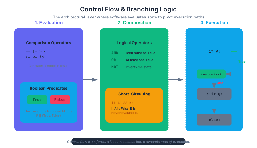
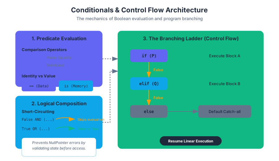
In the realm of computational theory, a program without branching is merely a list—a linear sequence of instructions that executes identically regardless of input. To transform a calculator into an autonomous agent, we require Conditionals and Branching. This is the architectural layer where software gains the ability to "decide," pivoting its execution path based on the state of the system or the nuances of user input.
At its core, branching is the implementation of Control Flow, the order in which individual statements, instructions, or function calls are executed. By evaluating the "truthiness" of specific expressions, a program can bypass certain blocks of code or repeat others, effectively creating a dynamic map of execution.
The Foundation: Boolean Expressions and Predicates
Before a program can branch, it must evaluate a condition. This evaluation results in a Boolean value—named after George Boole, who defined an algebraic system of logic in the mid-19th century. In modern computing, a Boolean expression (or predicate) is any statement that resolves to exactly one of two states: True or False.
The Law of the Excluded Middle
In classical logic, the Law of the Excluded Middle states that for any proposition, either that proposition is true, or its negation is true. In programming, we use this to ensure that our branching logic is exhaustive and deterministic.
Definition: Boolean Expression A formal representation of a truth-value, denoted as $P \in {True, False}$. In a programming context, this is often the result of a comparison between two variables or a variable and a literal.
Comparison Operators: The Mechanics of Evaluation
To generate Boolean values, we utilize Comparison Operators. These operators act as the bridge between raw data and logical decisions. While they appear simple, their implementation varies across languages, particularly regarding type coercion and identity.
| Operator | Name | Mathematical Symbol | Description | Example (Python) |
|---|---|---|---|---|
== |
Equality | $=$ | Returns True if values are equivalent |
5 == 5.0 (True) |
!= |
Inequality | $\neq$ | Returns True if values are different |
"a" != "b" (True) |
> |
Greater Than | $>$ | True if left is strictly greater than right | 10 > 5 (True) |
< |
Less Than | $<$ | True if left is strictly less than right | 2 < -1 (False) |
>= |
Greater or Equal | $\geq$ | True if left is greater than or equal to right | 5 >= 5 (True) |
<= |
Less or Equal | $\leq$ | True if left is less than or equal to right | 3 <= 4 (True) |
Value vs. Identity
A common pitfall for senior engineers is confusing Value Equality (==) with Identity Equality (is in Python, === in some contexts).
- Value Equality: Do these two objects represent the same data?
- Identity Equality: Do these two variables point to the exact same memory address?
# Code Block 1: Low-level implementation of a validation engine
# Language: Python
# Purpose: Demonstrates complex conditional logic and identity vs value

def validate_transaction(account_id, amount, security_token):
    """
    Validates a financial transaction using multi-stage branching.
    """
    MIN_BALANCE = 100.0
    SYSTEM_TOKEN = "SECRET_HEX_0x45"

    # 1. Identity check (Security)
    if security_token is not SYSTEM_TOKEN:
        # Note: In Python, small strings are interned, but for
        # security, we'd usually use a constant-time comparison.
        return "ERROR: Invalid Security Identity"

    # 2. Value comparison (Business Logic)
    if amount <= 0:
        return "ERROR: Transaction amount must be positive"

    # 3. State-based branching
    current_balance = get_balance_from_db(account_id)

    if current_balance - amount < MIN_BALANCE:
        # Branching based on a calculated predicate
        return "ERROR: Insufficient funds to maintain minimum balance"
    else:
        # The 'Happy Path'
        process_funds(account_id, amount)
        return "SUCCESS: Transaction Complete"

def get_balance_from_db(uid): return 500.0 # Mock
def process_funds(uid, amt): pass # Mock
Logical Operators: Composing Complexity
Rarely is a decision based on a single factor. We use Logical Operators to combine multiple Boolean expressions into a single compound condition.
- AND (
and): ReturnsTrueonly if both operands are true. - OR (
or): ReturnsTrueif at least one operand is true. - NOT (
not): Reverses the Boolean state (Unary operator).
Truth Tables for Logical Composition
| A | B | A AND B | A OR B | NOT A |
|---|---|---|---|---|
| True | True | True | True | False |
| True | False | False | True | False |
| False | True | False | True | True |
| False | False | False | False | True |
Short-Circuit Evaluation
Modern compilers and interpreters optimize logical expressions via Short-Circuiting.
- In an
ANDoperation, if the first operand isFalse, the entire expression is immediatelyFalse, and the second operand is never evaluated. - In an
ORoperation, if the first operand isTrue, the entire expression is immediatelyTrue.
This is critical for preventing errors. For example: if (obj != null && obj.isActive()). Without short-circuiting, calling obj.isActive() on a null object would crash the program.
Branching Structures: if, elif, and else
The if statement is the primary mechanism for branching. It evaluates a predicate and, if true, executes the indented block of code.
The if-elif-else Ladder
When multiple mutually exclusive conditions exist, we use the elif (else-if) structure. This is more efficient than nested if statements because the program stops checking conditions as soon as one evaluates to True.
f(x) =
\begin{cases}
\text{Action A} & \text{if } x > 0 \\
\text{Action B} & \text{if } x < 0 \\
\text{Action C} & \text{otherwise}
\end{cases}
Pseudocode Representation of Multi-way Branching
// Code Block 2: Pseudocode for a Traffic Control Algorithm
// Purpose: Illustrating the logic flow of an if-elif-else structure

ALGORITHM TrafficLightControl(sensor_data):
    IF sensor_data.emergency_vehicle_detected IS true THEN
        SET light_status TO "RED" FOR ALL directions
        SET emergency_lane TO "GREEN"
    ELSE IF sensor_data.pedestrian_waiting IS true AND sensor_data.timer > 30 THEN
        SET light_status TO "YELLOW"
        WAIT 3 seconds
        SET light_status TO "RED"
        ACTIVATE pedestrian_walk_signal
    ELSE IF sensor_data.car_count > 10 THEN
        EXTEND green_light_duration BY 15 seconds
    ELSE
        MAINTAIN default_cycle
    END IF
END ALGORITHM
Nested Conditionals and Cyclomatic Complexity
A Nested Conditional is an if statement located inside the block of another if statement. While powerful, excessive nesting leads to "Spaghetti Code" and high Cyclomatic Complexity—a metric used to measure the number of linearly independent paths through a program's source code.
Theorem: The Arrow Anti-pattern Code that heavily utilizes nested conditionals often forms a "shape" like an arrow pointing to the right. This is generally considered a sign that the logic should be refactored into guard clauses or a lookup table.
Advanced Branching: Switch and Pattern Matching
In many languages (C, Java, JavaScript), the switch statement provides a cleaner way to branch based on the value of a single variable. In Python 3.10+, this was introduced as Structural Pattern Matching using match and case.
Performance Comparison: If-Else vs. Switch
| Feature | If-Else Ladder | Switch / Match |
|---|---|---|
| Execution | Linear ($O(N)$) | Often Jump Table ($O(1)$) |
| Flexibility | Any Boolean expression | Usually discrete values/patterns |
| Readability | Poor for many conditions | High for many conditions |
| Use Case | Ranges, complex logic | Enumerations, specific constants |
/* Code Block 3: Low-level branching in C */
/* Purpose: Demonstrates the 'switch' statement and fall-through behavior */

#include <stdio.h>

void process_status(int status_code) {
    switch (status_code) {
        case 200:
            printf("OK: Request successful.\n");
            break;
        case 404:
            printf("Error: Resource not found.\n");
            break;
        case 500:
        case 503:
            /* Fall-through: both 500 and 503 execute this block */
            printf("Critical: Server-side failure.\n");
            break;
        default:
            printf("Unknown Status Code.\n");
    }
}
Real-World Application: Configuration and DevOps
Branching isn't limited to application code; it is fundamental to infrastructure as code (IaC) and CI/CD pipelines. Here, conditionals determine which environment to deploy to or which tests to run.
# Code Block 4: Conditional Logic in GitHub Actions (YAML)
# Purpose: Real-world usage of conditionals in a DevOps pipeline

jobs:
  deploy:
    runs-on: ubuntu-latest
    # Conditional: Only run this job if the push was to the 'main' branch
    if: github.ref == 'refs/heads/main'
    steps:
      - name: Checkout code
        uses: actions/checkout@v2

      - name: Deploy to Production
        run: |
          echo "Deploying to production server..."
          ./deploy_script.sh --env=prod
Common Pitfalls and Edge Cases
Even experienced developers fall prey to subtle logic errors when implementing branches.
1. The Floating Point Trap
Never use == with floating-point numbers. Due to binary precision limits, 0.1 + 0.2 does not exactly equal 0.3.
- Solution: Check if the absolute difference is less than a small epsilon:
abs(a - b) < 1e-9.
2. Assignment vs. Equality
In languages like C or Java, using = (assignment) instead of == (equality) inside an if statement is a valid syntax but a logical disaster.
- Example:
if (x = 5)setsxto 5 and then evaluates toTrue.
3. Algorithmic Bias
Conditionals encode the developer's assumptions. If a conditional structure in a hiring algorithm filters out candidates based on a "years of experience" threshold without considering non-traditional paths, it introduces Algorithmic Bias. Branching logic must be audited for fairness and inclusivity.
| Pitfall | Description | Corrective Action |
|---|---|---|
| Dangling Else | Ambiguity in nested if/else logic | Use explicit braces {} or indentation |
| Redundant Checks | Checking if (x == True) |
Use if x: directly |
| Dead Code | A branch that can never be reached | Use static analysis tools to prune |
| Over-nesting | Logic buried 5+ levels deep | Use "Guard Clauses" to return early |
Summary of Best Practices
- Favor Readability: If an
ifstatement has more than three conditions, break them into named Boolean variables. - Return Early: Use guard clauses to handle errors or edge cases at the top of a function, reducing the need for an
elseblock. - Be Explicit: Use parentheses to group logical operations, even if operator precedence makes them optional.
- Avoid Magic Numbers: Use named constants instead of raw numbers in comparisons (e.g.,
if status == STATUS_ACTIVEinstead ofif status == 1).
Logical Operators and Algorithmic Bias
Key concepts: Logical operators (AND, OR, NOT) · Nested conditionals · Algorithmic bias
Combining multiple conditions and exploring the ethical implications of automated decision-making.
Logical Operators and Algorithmic Bias
In the realm of computational logic, the transition from simple binary states to complex decision-making systems is mediated by Logical Operators and Nested Conditionals. While these tools allow us to construct sophisticated software, they also serve as the architecture through which Algorithmic Bias is codified. As we move from basic "if-then" statements to multi-layered decision trees, the precision of our logic determines not only the efficiency of the program but also the fairness of its outcomes.
The Mechanics of Boolean Logic: Logical Operators
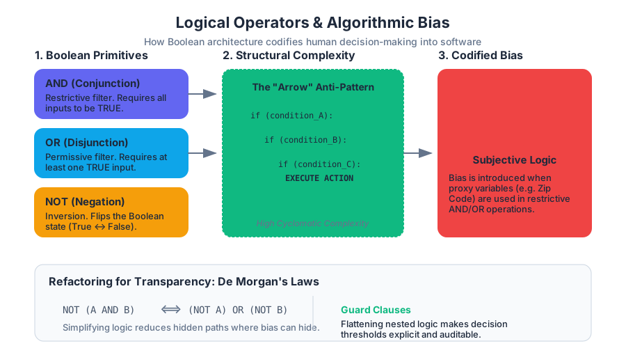
At the foundational level, logical operators allow a program to evaluate multiple conditions simultaneously. In Boolean algebra, these are known as conjunction (AND), disjunction (OR), and negation (NOT). These operators take Boolean inputs (True or False) and return a single Boolean result based on defined truth tables.
The Primary Operators
- AND (
&&orand): The result isTrueonly if all operands are true. It is used to narrow down possibilities, acting as a restrictive filter. - OR (
||oror): The result isTrueif at least one operand is true. It is used to broaden possibilities, acting as a permissive filter. - NOT (
!ornot): A unary operator that inverts the Boolean value.TruebecomesFalse, and vice versa.
The Principle of Short-Circuit Evaluation: Modern compilers and interpreters often use short-circuiting to optimize performance. In an
ANDoperation, if the first condition isFalse, the second is never evaluated because the overall result cannot possibly beTrue. Conversely, in anORoperation, if the first condition isTrue, the second is skipped.
Truth Table Comparison
| Operator | Input A | Input B | Result | Logical Name |
|---|---|---|---|---|
| AND | True | True | True | Conjunction |
| AND | True | False | False | Conjunction |
| OR | True | False | True | Disjunction |
| OR | False | False | False | Disjunction |
| NOT | True | N/A | False | Negation |
| XOR | True | True | False | Exclusive OR |
Implementation in Pythonic Logic
The following example demonstrates a high-level risk assessment algorithm using logical operators to determine if a transaction should be flagged for manual review.
def evaluate_transaction_risk(amount, is_international, account_age_days, failed_attempts):
    """
    Determines if a financial transaction requires an MFA challenge.
    Demonstrates the use of AND, OR, and NOT in a production context.
    """
    # Constants for business logic
    HIGH_VALUE_THRESHOLD = 10000
    NEW_ACCOUNT_THRESHOLD = 30
    MAX_FAILED_ATTEMPTS = 3

    # Logic: Flag if (High value AND New account) OR (Too many failed attempts)
    # OR if it's an international transaction NOT from a trusted age account.

    is_high_risk_new_user = (amount > HIGH_VALUE_THRESHOLD) and (account_age_days < NEW_ACCOUNT_THRESHOLD)
    has_security_red_flags = (failed_attempts >= MAX_FAILED_ATTEMPTS)
    is_suspicious_intl = is_international and not (account_age_days > 365)

    if is_high_risk_new_user or has_security_red_flags or is_suspicious_intl:
        return "FLAG_FOR_MFA"

    return "APPROVE_TRANSACTION"

# Example usage
print(evaluate_transaction_risk(12000, False, 15, 0)) # Output: FLAG_FOR_MFA
Nested Conditionals and Structural Complexity
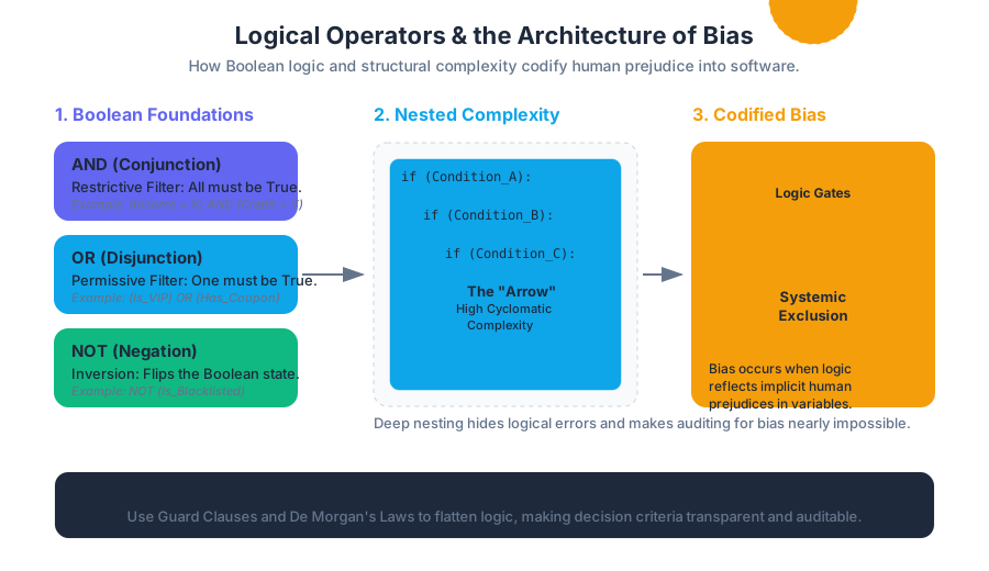
When a single line of logic is insufficient to capture the nuances of a problem, programmers employ Nested Conditionals. This involves placing an if statement inside the block of another if statement. While powerful, nesting increases the Cyclomatic Complexity of the code—a metric used to measure the number of linearly independent paths through a program's source code.
The "Arrow Anti-pattern"
Deep nesting often leads to what is colloquially known as the "Arrow Anti-pattern," where the code indentation forms a shape resembling an arrowhead. This makes code significantly harder to debug and audit, which is a primary breeding ground for logical errors and hidden biases.
Formalizing Logic with De Morgan's Laws
To reduce nesting and simplify complex Boolean expressions, we use De Morgan's Laws. These laws allow us to transform "NOT (A AND B)" into "(NOT A) OR (NOT B)".
\begin{aligned}
\neg(P \land Q) \iff (\neg P) \lor (\neg Q) \\
\neg(P \lor Q) \iff (\neg P) \land (\neg Q)
\end{aligned}
Comparison: Nested vs. Flattened Logic
| Feature | Nested Conditionals | Flattened (Guard Clauses) |
|---|---|---|
| Readability | Low (Deep indentation) | High (Linear flow) |
| Auditability | Difficult to trace paths | Easy to verify conditions |
| Complexity | High Cyclomatic Complexity | Lower per-function complexity |
| Error Proneness | High (Easy to miss an else) |
Low (Explicit exits) |
Refactoring for Clarity
Below is a mathematical representation of how a nested logic structure can be simplified using Boolean identities to improve transparency.
ORIGINAL NESTED LOGIC:
IF (user.is_authenticated):
    IF (user.has_permission):
        IF (resource.is_available):
            GRANT ACCESS
        ELSE:
            DENY (Unavailable)
    ELSE:
        DENY (No Permission)
ELSE:
    DENY (Unauthenticated)

SIMPLIFIED FLAT LOGIC (Guard Clauses):
IF NOT (user.is_authenticated) RETURN DENY
IF NOT (user.has_permission) RETURN DENY
IF NOT (resource.is_available) RETURN DENY
GRANT ACCESS
Algorithmic Bias: The Ghost in the Logic
Algorithmic Bias occurs when a computer system reflects the implicit values or prejudices of the humans who involved in its creation or the data used to train it. While we often think of "logic" as objective, the choice of which variables to include in an AND statement or where to set the threshold in a comparison operator is a subjective decision with real-world consequences.
Sources of Bias in Logic Design
Bias is rarely the result of a "malicious line of code." Instead, it emerges from three primary areas:
- Representative Bias: The training data does not accurately represent the population.
- Proxy Variables: Using a variable that seems neutral but correlates strongly with a protected characteristic (e.g., using "Zip Code" as a proxy for race).
- Threshold Bias: Setting logical cut-offs that disproportionately affect specific groups.
Case Study: The "False Negative" in Loan Approvals
Consider an algorithm designed to approve small business loans. The logic might look like this:
IF (credit_score > 700 AND annual_revenue > 50000) THEN APPROVE.
On the surface, this is "neutral" math. However, if historical systemic factors have prevented certain demographics from building traditional credit scores, the AND operator acts as a hard gate that reinforces historical inequality, even if the individual is currently credit-worthy.
Common Types of Algorithmic Bias
| Bias Type | Definition | Example in Logic |
|---|---|---|
| Historical Bias | Data reflects past prejudices. | Hiring logic based on "successful" past employees. |
| Measurement Bias | Tools measure data inconsistently. | Facial recognition failing on darker skin tones due to sensor settings. |
| Aggregation Bias | One-size-fits-all logic for diverse groups. | Health risk scores that ignore ethnic variations in biomarkers. |
| Evaluation Bias | The benchmark used to test the logic is flawed. | Testing a "universal" UI only on users with high-speed internet. |
Auditing Logic for Fairness
To combat bias, engineers must move beyond "functional" testing (does the code work?) to "adversarial" or "fairness" testing (who does this code fail?). This involves querying the data and the logic to find disparate impacts.
Detecting Proxy Variables with SQL
A common task for a data engineer is to audit a database to see if certain logical filters are inadvertently targeting protected groups.
-- Auditing for Disparate Impact
-- This query checks if a "High Risk" flag correlates disproportionately
-- with a specific demographic, even if that demographic isn't in the logic.

SELECT
    demographic_group,
    COUNT(*) AS total_users,
    SUM(CASE WHEN risk_score > 0.8 THEN 1 ELSE 0 END) AS flagged_users,
    (SUM(CASE WHEN risk_score > 0.8 THEN 1 ELSE 0 END) * 1.0 / COUNT(*)) AS flag_rate
FROM
    user_data
JOIN
    outcomes ON user_data.id = outcomes.user_id
GROUP BY
    demographic_group
HAVING
    flag_rate > (SELECT AVG(flag_rate) * 1.2 FROM outcomes);
    -- Flags groups with 20% higher rate than average
Technical Mitigation Strategies
- Individual Fairness: Ensuring that similar individuals receive similar outcomes.
- Group Fairness (Statistical Parity): Ensuring the percentage of "True" outcomes is equal across different demographic groups.
- Counterfactual Fairness: A logic gate is fair if the outcome would be the same if a protected attribute (like gender) were changed, holding all other factors constant.
Theorem: The Impossibility of Fairness Mathematical proofs (notably by Kleinberg et al.) have shown that it is often impossible to satisfy all definitions of fairness simultaneously. For example, you cannot usually achieve both "Predictive Parity" and "Equalized Odds" if the base rates of a condition differ between groups. This makes the "logic" of ethics a series of trade-offs rather than a single solvable equation.
Advanced Implementation: Auditing via CLI
In a DevOps or MLOps pipeline, we might use a CLI tool to check a model's fairness metrics before deployment.
# Example: Using a hypothetical fairness-audit CLI tool
# This checks a model (v2_hiring_logic) against a test dataset (census_data.csv)
# looking for violations of the "Four-Fifths Rule" (Impact Ratio < 0.8)

audit-fairness --model ./models/v2_hiring_logic.bin \
               --data ./data/census_data.csv \
               --protected-attr "ethnicity" \
               --target-result "hired" \
               --threshold 0.8

# Output:
# [WARNING] Disparate Impact detected in Group 'C'.
# Impact Ratio: 0.62 (Below threshold 0.8)
# Recommendation: Review logical weights for 'years_of_uninterrupted_employment'.
Summary of Best Practices
To master logical operators while minimizing bias, developers should adhere to the following principles:
- Prefer Guard Clauses: Instead of deep nesting, use early returns to handle edge cases. This makes the "happy path" of the logic visible and auditable.
- Explicit over Implicit: Avoid complex "one-liners" that combine five different
AND/ORconditions. Break them into descriptive Boolean variables. - Audit the "Else": Bias often hides in the
elseblock—the default action taken when a user doesn't meet specific (often privileged) criteria. - Contextualize Thresholds: Be aware that a "hard limit" (e.g.,
age > 18) is a logical choice that may require exceptions or "soft" logic in different cultural or legal contexts.
Conclusion
Logical operators are the grammar of computation, and nested conditionals are its complex sentences. However, as we have seen, the "truth" of a Boolean expression is only as objective as the parameters we define. By understanding the mechanics of AND, OR, and NOT, and by remaining vigilant against the structural pitfalls of nested logic and algorithmic bias, we can build systems that are not only technically sound but socially responsible. Logic is a tool for precision; ethics is the guide for its application.
Loops and Repetition
Key concepts: While loops · For loops · range() function
Using loops to automate repetitive tasks and manage program flow.
Loops and Repetition
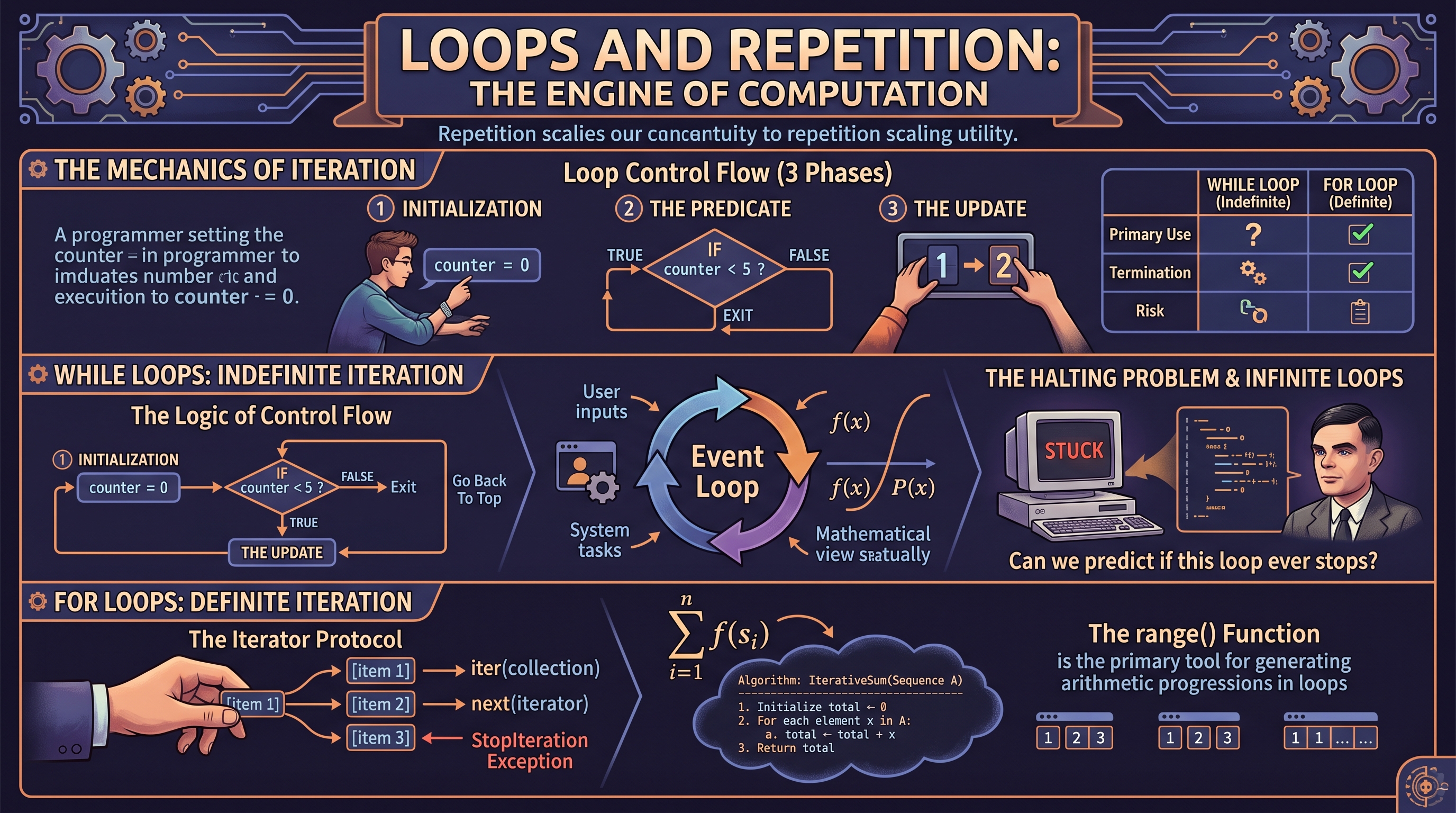
In the architecture of computation, repetition is the engine of utility. While conditional logic allows a program to "choose," loops allow a program to "scale." At its core, a loop is a control flow structure that executes a statement or a block of statements multiple times, either until a specific condition is met or until every element in a collection has been processed.
Without loops, the utility of a computer would be limited to the speed at which a human could write individual lines of code. With loops, we leverage the fundamental advantage of silicon over biology: the ability to perform billions of discrete, identical operations with zero fatigue and absolute precision.
The Mechanics of Iteration
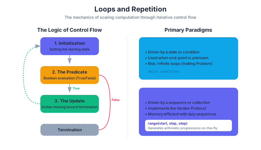
Iteration is the process of repeatedly executing a set of instructions. In high-level languages like Python, this is abstracted into two primary forms: indefinite iteration (where the number of repetitions is not known beforehand) and definite iteration (where the number of repetitions is predetermined).
The Logic of Control Flow
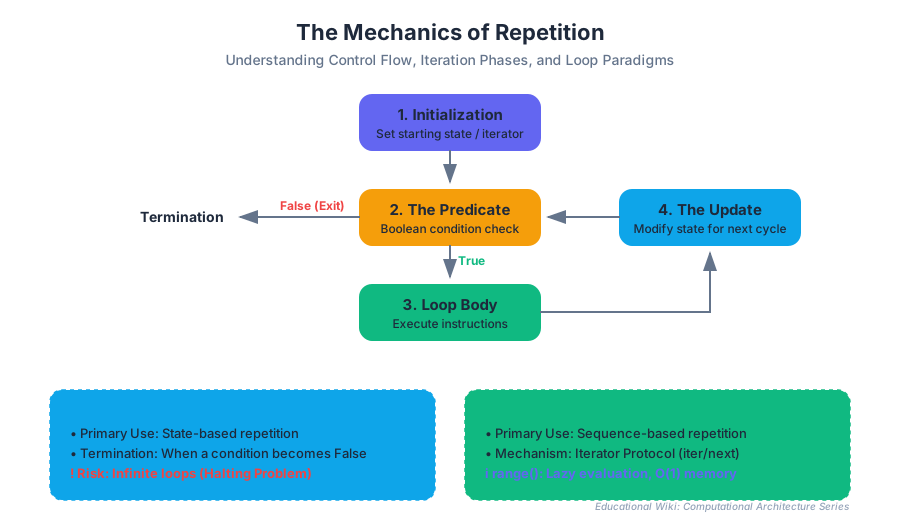
Every loop consists of three conceptual phases:
- Initialization: Setting the starting state or the iterator.
- The Predicate (Condition): A Boolean evaluation that determines if the loop should continue.
- The Update (Side Effect): An action that moves the state closer to the termination condition.
| Feature | While Loop (Indefinite) | For Loop (Definite) |
|---|---|---|
| Primary Use | State-based repetition | Sequence-based repetition |
| Termination | When a condition becomes False |
When the sequence is exhausted |
| Risk | Infinite loops (Non-termination) | Index errors (less common in Python) |
| Memory | Minimal (stores only state) | Depends on the sequence size |
While Loops: Indefinite Iteration
A While Loop is the most fundamental form of repetition. It mirrors the logical structure of an if statement but returns to the top of the block after each execution. Mathematically, it can be viewed as a recursive function $f(x)$ that continues as long as $P(x)$ is true.
Definition: The While Loop A control structure that repeatedly executes a target statement as long as a given condition (the predicate) evaluates to
True.
Why It Matters
While loops are essential when the termination point depends on external factors—user input, a sensor reading, or a mathematical convergence—rather than a fixed count. In systems programming, the "Event Loop" is a perpetual while loop that keeps an operating system or application running.
Implementation and Memory
In low-level terms, a while loop is a combination of a comparison and a jump instruction.
// First code block: Low-level implementation in C
// Demonstrating the assembly-like logic of a while loop
#include <stdio.h>

int main() {
    int counter = 0;
    int threshold = 1000;

    // The loop header performs a comparison
    while (counter < threshold) {
        // Body of the loop
        if (counter % 100 == 0) {
            printf("Processing checkpoint: %d\n", counter);
        }

        // The Update: Critical to avoid infinite loops
        counter++;
    }
    // After the jump: condition is now false
    return 0;
}
The Halting Problem
A significant risk with while loops is the Infinite Loop. If the predicate never evaluates to False, the program enters a state of non-termination. This relates to Alan Turing’s "Halting Problem," which proves that there is no general algorithm that can determine, for any program and input, whether the program will eventually stop.
For Loops: Definite Iteration
A For Loop is designed to iterate over a pre-defined collection or sequence. In Python, the for loop is actually an implementation of the Iterator Pattern, which abstracts the process of moving through a data structure.
The Iterator Protocol
When you write for item in collection:, Python performs the following behind the scenes:
- Calls
iter(collection)to get an iterator object. - Repeatedly calls
next(iterator)to retrieve the next value. - Catches the
StopIterationexception to terminate the loop gracefully.
\text{For a set } S = \{s_1, s_2, \dots, s_n\}, \text{ a for loop computes: } \\
\sum_{i=1}^{n} f(s_i) \text{ or } \prod_{i=1}^{n} f(s_i)
Mathematical Derivation of Iteration
We can represent the state change in a loop using recurrence relations. If $x_n$ is the state after $n$ iterations:
Second code block: Mathematical representation and Pseudocode
Algorithm: IterativeSum(Sequence A)
----------------------------------
1. Initialize total ← 0
2. For each element x in A:
    a. total ← total + x
3. Return total

Mathematical Recurrence:
S[0] = 0
S[i] = S[i-1] + A[i]  for i > 0
The range() Function
The range() function is the primary tool for generating arithmetic progressions in Python. Unlike a list, range is a lazy sequence (an immutable sequence type). It does not store all numbers in memory; instead, it calculates them on the fly.
Parameters and Complexity
The range() function accepts up to three arguments: start, stop, and step.
| Parameter | Role | Default |
|---|---|---|
start |
The starting integer of the sequence | 0 |
stop |
The upper bound (exclusive) | Required |
step |
The increment between each number | 1 |
Insight: Memory Efficiency Because
rangeis a generator-like object,range(0, 1000000)takes the same amount of memory asrange(0, 10), regardless of the size of the range. It only stores the start, stop, and step values.
Practical Usage
range() is frequently used to iterate a specific number of times or to access elements by their index.
# Third code block: Real-world usage in Python
# Simulating a population growth model using range() and randomness
import random

def simulate_population(initial_pop, growth_rate, generations):
    population = initial_pop
    print(f"Starting Simulation: {population} individuals")

    for gen in range(1, generations + 1):
        # Apply growth rate with a random environmental factor
        factor = random.uniform(0.9, 1.1)
        population = int(population * growth_rate * factor)

        # Logging results every 5 generations
        if gen % 5 == 0:
            print(f"Generation {gen}: Population = {population}")

    return population

final_count = simulate_population(100, 1.05, 20)
Loop Control Flow: Break and Continue
Sometimes, the standard entry/exit points of a loop are insufficient. Control flow statements allow for more granular movement within the loop body.
break: Immediately terminates the loop and jumps to the first line of code after the loop block.continue: Skips the remainder of the current iteration and jumps back to the top of the loop (the predicate or next sequence item).else(Python specific): A unique clause that executes only if the loop finished "naturally" (i.e., it did not encounter abreak).
Control Statement Comparison
| Statement | Effect on Current Iteration | Effect on Loop State | Common Use Case |
|---|---|---|---|
break |
Terminated | Entire loop exits | Searching for an item (Early exit) |
continue |
Terminated | Moves to next iteration | Skipping invalid data/noise |
pass |
None (No-op) | Continues normally | Placeholder for future code |
Nested Loops and Algorithmic Complexity
A Nested Loop occurs when a loop is placed inside the body of another loop. This is common in processing multi-dimensional data, such as matrices or coordinate systems.
The Cost of Nesting
Nesting loops significantly impacts the Time Complexity of an algorithm.
- A single loop over $n$ items is $O(n)$ (Linear time).
- A loop over $n$ items inside another loop over $n$ items is $O(n^2)$ (Quadratic time).
# Fourth code block: Shell script demonstrating nested iteration
# Generating a grid of coordinates for a batch processing task
#!/bin/bash

ROWS=3
COLS=4

echo "Generating $ROWS x $COLS grid..."

for ((i=1; i<=ROWS; i++))
do
    for ((j=1; j<=COLS; j++))
    do
        printf "(%d,%d) " $i $j
    done
    echo "" # Newline after each row
done
Common Pitfalls and Best Practices
Even experienced engineers encounter subtle bugs when implementing repetition logic.
1. The Off-by-One Error
This occurs when a loop iterates one time too many or one time too few. This is often caused by confusion between inclusive and exclusive bounds (e.g., range(0, 10) stops at 9).
2. Modifying a Collection While Iterating
In many languages, including Python, adding or removing items from a list while you are looping over it can lead to skipped elements or runtime errors.
- Solution: Iterate over a copy of the list (
for item in my_list[:]) or collect items to be removed in a separate list and process them afterward.
3. Floating Point Precision in Predicates
Using floating-point numbers in a while loop condition is dangerous due to precision issues.
- Bad:
while x != 1.0:(x might become 0.99999999 and skip 1.0). - Good:
while x < 1.0:orwhile abs(x - 1.0) > 1e-9:.
Advanced Pattern: The Accumulator Pattern
The Accumulator Pattern is a common algorithmic design where a variable (the accumulator) is updated in every iteration of a loop to maintain a running total, a concatenated string, or a filtered list.
# Fifth code block: Accumulator Pattern in Data Modeling
# Filtering a dictionary of sensor data and calculating an average

sensor_data = {
    "sensor_a": 22.5,
    "sensor_b": None,
    "sensor_c": 25.8,
    "sensor_d": 19.2,
    "sensor_e": "Error"
}

def calculate_clean_average(data):
    total = 0.0      # Accumulator 1: Sum
    count = 0        # Accumulator 2: Count

    for sensor, value in data.items():
        # Type checking to ensure we only process floats/ints
        if isinstance(value, (int, float)):
            total += value
            count += 1
        else:
            print(f"Skipping invalid data at {sensor}: {value}")

    return total / count if count > 0 else 0

avg = calculate_clean_average(sensor_data)
print(f"Average Temperature: {avg:.2f}")
Summary of Loop Types
| Loop Type | Best For... | Key Syntax (Python) |
|---|---|---|
| For-in | Iterating over lists, strings, or dicts | for item in collection: |
| For-range | Repeating an action $N$ times | for i in range(n): |
| While | Waiting for a condition to change | while condition: |
| Nested | Multi-dimensional arrays/grids | for x in row: for y in col: |
Conclusion
Loops are the primary mechanism for scaling logic. Whether you are traversing a simple list with a for loop, managing a complex state machine with a while loop, or generating efficient numeric sequences with range(), understanding the underlying mechanics of iteration is vital. By mastering control flow statements and being mindful of algorithmic complexity, you can write code that is not only functional but also performant and robust.
Simulations and Control Flow
Key concepts: Break and Continue · Randomness · Simulating natural selection
Controlling loop execution and using randomness to simulate real-world phenomena.
Simulations and Control Flow
In the architecture of computational logic, the transition from static scripts to dynamic simulations represents a fundamental leap in complexity. While basic algorithms follow a linear or strictly branching path, Simulations allow us to model the stochastic (random) and iterative nature of reality. To build these models, we must master the fine-grained control of execution flow—specifically how to interrupt, skip, or terminate cycles—and how to inject controlled entropy through randomness.
This section dissects the mechanics of loop control, the mathematical foundations of pseudo-randomness, and the implementation of biological heuristics through simulated natural selection.
The Mechanics of Interruption: Break and Continue
In standard iterative logic, a loop executes its block until a condition is met. However, real-world data is often "noisy" or contains early-exit triggers. To handle these, we employ non-local control flow statements: break and continue. These are not merely "shortcuts"; they are essential tools for optimizing algorithmic complexity and maintaining clean code architecture.
1. The break Statement: Immediate Termination
The break statement provides an "emergency exit" from the innermost loop. When the interpreter encounters break, it immediately halts the loop's execution and jumps to the first line of code following the loop block.
- Mathematical Motivation: In search algorithms, once the target element $x$ is found in set $S$, further iterations are $O(n)$ waste.
breakallows us to achieve an average-case performance of $O(n/2)$ rather than forcing $O(n)$. - The Sentinel Pattern:
breakis frequently used in "infinite" loops (while True) where the exit condition is complex or depends on external input that cannot be evaluated at the loop's header.
2. The continue Statement: Iterative Skipping
Unlike break, continue does not terminate the loop. Instead, it "short-circuits" the current iteration, skipping the remaining code in the block and jumping directly to the next evaluation of the loop condition (in while loops) or the next element (in for loops).
- The Guard Clause Pattern:
continueis used to avoid deeply nestedifstatements (the "Arrow Anti-pattern"). By checking for invalid data at the top of a loop and usingcontinue, the "happy path" of the code remains at a low indentation level.
| Statement | Scope | Effect on Loop | Post-Execution Pointer |
|---|---|---|---|
break |
Innermost loop | Terminates loop immediately | First line after the loop block |
continue |
Innermost loop | Skips current iteration | Next iteration/condition check |
pass |
Any block | No effect (placeholder) | Next line in the same block |
return |
Function | Terminates function | Back to the caller |
Implementation: Low-Level Control Flow in C
To understand how these work under the hood, we look at the assembly-like behavior in C, where these statements translate to JMP (jump) instructions in the CPU.
#include <stdio.h>

/**
 * Demonstrates a robust search and filter simulation.
 * We search for a target value but skip "noisy" data (negative numbers).
 */
int main() {
    int data[] = {10, -5, 20, 33, -1, 40, 50};
    int target = 33;
    int size = sizeof(data) / sizeof(data[0]);

    for (int i = 0; i < size; i++) {
        // 1. Noise Filtering (Continue)
        if (data[i] < 0) {
            printf("Skipping noise at index %d\n", i);
            continue;
        }

        // 2. Target Identification (Break)
        if (data[i] == target) {
            printf("Target %d found at index %d. Terminating search.\n", target, i);
            break;
        }

        printf("Processing valid data: %d\n", data[i]);
    }
    return 0;
}
The Architecture of Randomness
Simulations require unpredictability. However, computers are inherently deterministic machines—given the same input and state, they will always produce the same output. To simulate "randomness," we use Pseudo-Random Number Generators (PRNGs).
What it is
A PRNG is an algorithm that uses mathematical formulas to produce sequences of numbers that appear random. These sequences are actually deterministic and originate from an initial value called a Seed.
The Determinism Theorem: If you know the seed and the algorithm of a PRNG, you can predict every subsequent number in the sequence with 100% accuracy.
Why it matters
In simulations, we use randomness to model:
- Stochastic Processes: Events that have a known probability but an uncertain outcome (e.g., a coin flip).
- Monte Carlo Methods: Using repeated random sampling to obtain numerical results (e.g., calculating the area under a curve).
- Variability: Ensuring that a simulation of a forest or a population doesn't result in identical "clones."
Mathematical Derivation: The Linear Congruential Generator (LCG)
Most basic random modules (like Python's random or C's rand()) are based on variations of the LCG. The formula for generating the next number $X_{n+1}$ is:
X_{n+1} = (aX_n + c) \pmod m
Where:
- $X$ is the sequence of pseudo-random values.
- $m$ is the "modulus" (the maximum range).
- $a$ is the "multiplier."
- $c$ is the "increment."
- $X_0$ is the Seed.
| Parameter | Constraint | Purpose |
|---|---|---|
m |
$m > 0$ | Defines the period length (how long before the sequence repeats). |
a |
$0 < a < m$ | Controls the "shuffling" of bits. |
c |
$0 \le c < m$ | Ensures the sequence doesn't get stuck at zero. |
seed |
$0 \le seed < m$ | The starting point of the sequence. |
Common Pitfalls: The Seed Trap
A common mistake is re-seeding the generator inside a loop. If you set the seed to the current system time inside a fast-running loop, the time may not change between iterations, causing the "random" generator to return the exact same number repeatedly. Always seed once at the start of the program.
Simulating Natural Selection
Natural selection is the ultimate biological algorithm. It is a process where individuals with favorable traits are more likely to reproduce, passing those traits to the next generation. In computer science, we model this using Genetic Algorithms (GAs).
The Simulation Pipeline
A simulation of natural selection follows a specific iterative loop:
- Initialization: Create a population of individuals with random traits (chromosomes).
- Fitness Evaluation: Calculate a "fitness score" for each individual based on how well they solve a specific problem.
- Selection: Choose the "parents" for the next generation, favoring those with higher fitness scores.
- Crossover (Recombination): Combine traits from two parents to create offspring.
- Mutation: Randomly flip or change a trait in the offspring to maintain genetic diversity.
- Replacement: Replace the old population with the new generation and repeat.
Concrete Example: The "String Evolution" Simulation
Imagine we want to evolve a random string of characters until it matches the target phrase "EVOLVE".
- Fitness: Number of characters in the correct position.
- Mutation Rate: The probability (e.g., 1%) that a character changes randomly.
Implementation: Python Population Simulation
This example uses a high-level approach to model a population evolving toward a target.
import random

# Configuration
TARGET = "EVOLVE"
ALPHABET = "ABCDEFGHIJKLMNOPQRSTUVWXYZ "
POP_SIZE = 100
MUTATION_RATE = 0.01

def get_fitness(genome):
    """Calculates how many characters match the target."""
    return sum(1 for g, t in zip(genome, TARGET) if g == t)

def mutate(genome):
    """Randomly alters a gene based on the mutation rate."""
    genome_list = list(genome)
    for i in range(len(genome_list)):
        if random.random() < MUTATION_RATE:
            genome_list[i] = random.choice(ALPHABET)
    return "".join(genome_list)

# 1. Initialization
population = ["".join(random.choice(ALPHABET) for _ in range(len(TARGET)))
              for _ in range(POP_SIZE)]

generation = 0
while True:
    generation += 1

    # 2. Evaluation & Selection (Sort by fitness)
    population.sort(key=get_fitness, reverse=True)
    best_individual = population[0]

    if get_fitness(best_individual) == len(TARGET):
        print(f"Gen {generation}: {best_individual} (Target Reached!)")
        break

    if generation % 10 == 0:
        print(f"Gen {generation}: {best_individual} | Fitness: {get_fitness(best_individual)}")

    # 3. Reproduction (Top 10% survive and breed)
    new_population = population[:10]
    while len(new_population) < POP_SIZE:
        parent = random.choice(population[:20]) # Select from top 20
        child = mutate(parent)
        new_population.append(child)

    population = new_population
Advanced Simulation Concepts: Distributions and Probabilities
In complex simulations, random.random() (which gives a uniform distribution between 0 and 1) is often insufficient. Real-world phenomena usually follow different statistical distributions.
1. Uniform Distribution
Every outcome in a range is equally likely.
- Use Case: Rolling a fair die, picking a random card.
- Python:
random.uniform(a, b)
2. Normal (Gaussian) Distribution
Most outcomes cluster around a mean, with fewer outcomes at the extremes (the "Bell Curve").
- Use Case: Simulating heights of a population, IQ scores, or measurement errors.
- Python:
random.gauss(mu, sigma)(wheremuis the mean andsigmais the standard deviation).
3. Exponential Distribution
Models the time between independent events occurring at a constant average rate.
- Use Case: Time between customers arriving at a store, or the decay of radioactive particles.
- Python:
random.expovariate(lambd)
| Distribution | Shape | Key Parameters | Simulation Application |
|---|---|---|---|
| Uniform | Flat | Min, Max | Random selection, basic chance |
| Normal | Bell-shaped | Mean ($\mu$), Std Dev ($\sigma$) | Natural traits, sensor noise |
| Exponential | Decaying curve | Rate ($\lambda$) | Queuing theory, failure rates |
| Binomial | Discrete peaks | Trials ($n$), Prob ($p$) | Success/Failure counts (e.g., coin flips) |
Real-World Usage: CLI Simulation Control
In production environments, simulations are often run from the command line with varying "seeds" to ensure results are statistically significant.
# Running a natural selection simulation with different seeds
# to observe the variance in convergence time.

for seed in {1..5}; do
  echo "Running Simulation with SEED: $seed"
  python3 evolution_sim.py --seed $seed --pop_size 500 --mutation 0.05 >> results.log
done

# Analyze the results
grep "Target Reached" results.log | awk '{sum+=$2} END {print "Average Generations:", sum/NR}'
Summary of Control Flow and Simulation Logic
To build a successful simulation, one must balance Control and Chaos.
- Control is provided by
breakandcontinue, allowing the program to react to specific states within an iteration. - Chaos (or Entropy) is provided by the
randommodule, allowing the program to explore a "state space" that the programmer did not explicitly define.
When these are combined in a loop, we create an Evolving System. The loop provides the passage of time, the control flow provides the "rules of physics," and the randomness provides the "genetic variation."
Common Pitfalls in Simulations
- Infinite Loops: Forgetting to include a
breakcondition or an increment in awhileloop, causing the simulation to hang. - Off-by-One Errors: In population indexing, especially when removing "dead" individuals from a list while iterating over it.
- Floating Point Precision: Using
==to compare random floats (e.g.,if random.random() == 0.5). Instead, use inequalities (e.g.,if random.random() < 0.5). - Bias in PRNGs: Using a low-quality generator for cryptographic or high-stakes financial simulations.
Study Guide: Simulations and Control Flow
I. Core Definitions
- Break: A keyword used to exit the current loop immediately, bypassing any remaining iterations.
- Continue: A keyword used to skip the rest of the current loop's body and move to the next iteration.
- PRNG (Pseudo-Random Number Generator): An algorithm that produces a sequence of numbers approximating the properties of random numbers.
- Seed: The starting value for a PRNG. Using the same seed produces the same sequence of numbers.
- Fitness Function: A specific objective function used to summarize how close a given design solution is to achieving the set aims.
II. Control Flow Logic
- Use
breakfor: Searching for a specific item, exiting on user command, or handling error states. - Use
continuefor: Filtering out invalid data, skipping "empty" iterations, or simplifying nested logic.
III. Simulation Steps (Natural Selection)
- Initialize a random population.
- Loop through generations:
- Evaluate fitness of each member.
- Select the best members to be parents.
- Crossover parent traits to create children.
- Mutate children slightly to maintain variety.
- Repeat until a solution is found or time runs out.
IV. Key Functions (Python random)
random.random(): Float between 0.0 and 1.0.random.randint(a, b): Integer between $a$ and $b$ (inclusive).random.choice(sequence): Pick one random element from a list/string.random.seed(x): Initialize the generator state.
V. Mathematical Concepts
- LCG Formula: $X_{n+1} = (aX_n + c) \pmod m$.
- Stochasticity: The quality of lacking any predictable order or plan; randomness.
- Convergence: The process where a simulation approaches a stable state or a correct solution over time.
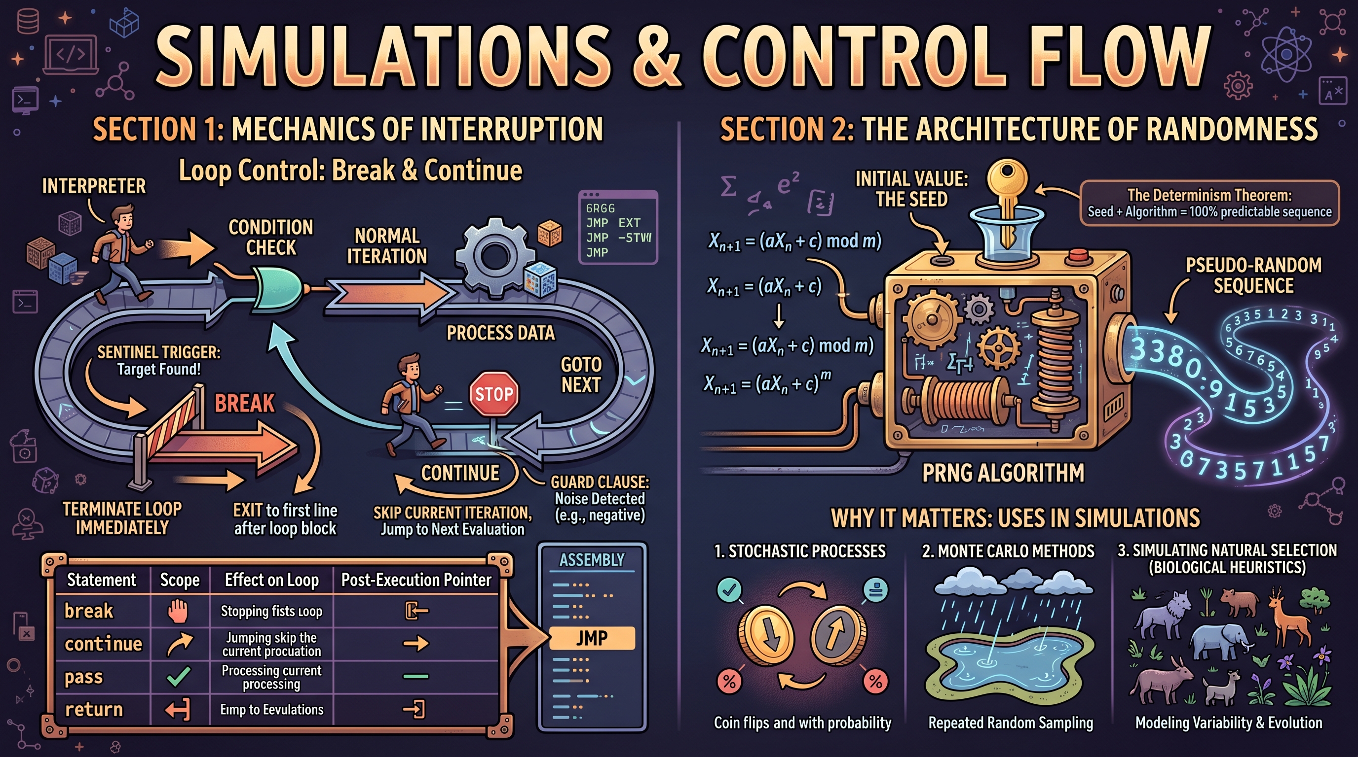
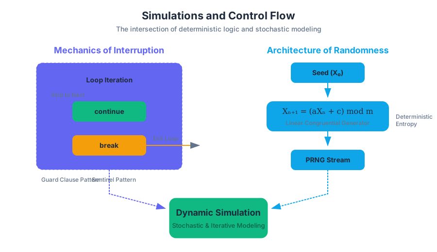
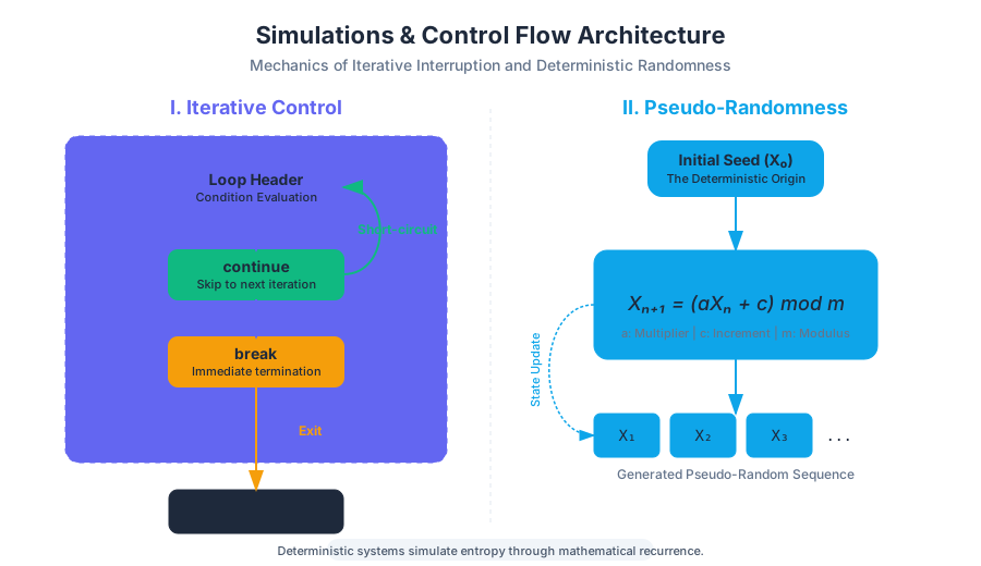
Functions and Modularity
Key concepts: Function definitions · Parameters · Return statements · Modularity
Organizing code into reusable, independent modules called functions.
Functions and Modularity
In the realm of software engineering, complexity is the primary antagonist. As a system grows, the cognitive load required to understand its state transitions and logic flow increases exponentially. To combat this, we employ Modularity: the architectural strategy of decomposing a monolithic problem into discrete, independent, and interchangeable sub-units. At the heart of modularity lies the Function.
A function is not merely a "block of code"; it is a formal abstraction. It represents a mapping from a set of inputs (the domain) to a set of outputs (the codomain), encapsulated in a way that hides implementation details from the caller. This principle, known as Abstraction, allows us to build "black boxes" where we care about what the code does, rather than how it does it.
The Anatomy of a Function Definition
A Function Definition is the blueprint for a computational task. In Python, this is initiated with the def keyword, followed by the function name, a parameter list, and a colon. This header defines the function's Signature—the contract it makes with the rest of the program.
The body of the function is an indented block of code. When a function is "called" or "invoked," the program's execution pointer jumps to this block, executes the logic, and then returns to the point of origin. This mechanism is managed by the Call Stack, a data structure that tracks active subroutines.
Definition: The Activation Record When a function is called, the system creates an Activation Record (or Stack Frame) on the call stack. This record contains the function's local variables, the arguments passed to it, and the return address. When the function finishes, its frame is "popped" off the stack, and its local memory is reclaimed.
Implementation: A Statistical Analysis Module
The following example demonstrates a non-trivial function designed to calculate the variance of a dataset. It showcases local variable encapsulation and algorithmic logic.
def calculate_variance(data_points: list[float]) -> float:
    """
    Calculates the population variance of a numeric dataset.
    Formula: σ² = Σ(x - μ)² / N
    """
    if not data_points:
        raise ValueError("Dataset cannot be empty.")

    # Step 1: Calculate the arithmetic mean (μ)
    n = len(data_points)
    mean = sum(data_points) / n

    # Step 2: Calculate the sum of squared differences from the mean
    squared_diff_sum = 0.0
    for x in data_points:
        diff = x - mean
        squared_diff_sum += diff ** 2

    # Step 3: Compute variance
    variance = squared_diff_sum / n
    return variance

# Execution context
observations = [10.5, 12.2, 9.8, 11.1, 10.9]
result = calculate_variance(observations)
print(f"Population Variance: {result:.4f}")
Formalizing the Mapping: Mathematical Representation
To understand functions at a fundamental level, we must look at them through the lens of discrete mathematics. A function $f$ is a relation that associates each element $x$ of a set $X$ to exactly one element $y$ of a set $Y$.
f: X \to Y
\text{where } x \in X \text{ is the input and } f(x) \in Y \text{ is the output.}
In programming, we extend this definition to include Side Effects—changes to the state of the system (like printing to a console or modifying a global variable) that occur during the function's execution. A Pure Function is one that has no side effects and always produces the same output for the same input, mirroring the mathematical ideal.
| Concept | Programming Definition | Mathematical Analog |
|---|---|---|
| Function Name | The identifier used to invoke the logic. | The symbol $f$ or $g$. |
| Parameters | Placeholders defined in the function header. | Variables in the expression (e.g., $x$ in $x^2$). |
| Arguments | The actual values passed during a call. | The specific value substituted (e.g., $f(5)$). |
| Return Value | The data sent back to the caller. | The result of the evaluation ($y$). |
| Scope | The visibility of variables. | The domain of the variable. |
Parameters and Arguments: The Input Interface
Parameters are the variables listed in the function's definition. They act as local names for the data the function expects. Arguments are the actual data values supplied to the function when it is called.
Parameter Passing Mechanisms
Different programming languages handle the transmission of arguments differently. Python uses a mechanism often called Pass-by-Object-Reference. This means the function receives a reference to the same object in memory, but the "name" in the function is local.
- Positional Arguments: Mapped to parameters based on their order.
- Keyword Arguments: Mapped by name, allowing for out-of-order passing.
- Default Parameters: Parameters that assume a pre-defined value if the caller provides none.
Comparison of Argument Types
| Type | Syntax Example | Use Case |
|---|---|---|
| Positional | power(2, 10) |
Simple, intuitive mappings. |
| Keyword | connect(host="localhost", port=8080) |
Improving readability in complex signatures. |
| Default | def log(msg, level="INFO"): |
Providing sensible defaults while allowing overrides. |
| *Variadic (args) | def sum_all(*nums): |
Functions that accept an arbitrary number of inputs. |
The Danger of Mutable Defaults
A common pitfall for senior and junior engineers alike is using mutable objects (like lists or dictionaries) as default arguments. In Python, default arguments are evaluated only once at the time of function definition, not at each call.
# ANTI-PATTERN: The list is shared across all calls!
def add_to_registry(name, registry=[]):
    registry.append(name)
    return registry

# CORRECT PATTERN: Use None as a sentinel
def add_to_registry_safe(name, registry=None):
    if registry is None:
        registry = []
    registry.append(name)
    return registry
Return Statements: The Output Pipeline
The return statement serves two purposes: it terminates the function's execution and optionally passes a value back to the calling environment. If a function reaches the end of its block without a return statement, it implicitly returns None.
Multiple Return Points
Functions can have multiple return statements, often used in "guard clauses" to handle edge cases early. This reduces the nesting level of the code (the "Arrow Anti-pattern").
Structural Comparison: Low-Level vs. High-Level Returns
To see how functions handle returns at a lower level, consider how a systems language like Rust manages ownership and return values compared to Python's reference-based approach.
// Rust implementation showing explicit return types and ownership
fn find_max(numbers: &[i32]) -> Option<i32> {
    if numbers.is_empty() {
        return None; // Early return for edge case
    }

    let mut max_val = numbers[0];
    for &val in numbers.iter() {
        if val > max_val {
            max_val = val;
        }
    }
    Some(max_val) // Final expression is returned implicitly in Rust
}

fn main() {
    let data = vec![1, 5, 3, 9, 2];
    match find_max(&data) {
        Some(max) => println!("The maximum is {}", max),
        None => println!("The list was empty"),
    }
}
Scope and the LEGB Rule
Scope defines the region of a program where a particular variable name is accessible. Understanding scope is critical for modularity because it prevents "Namespace Pollution"—where different parts of a program accidentally overwrite each other's data.
Python follows the LEGB Rule for variable resolution:
- L (Local): Names assigned within a function and not declared global.
- E (Enclosing): Names in the local scope of any enclosing functions (relevant in nested functions).
- G (Global): Names assigned at the top-level of a module or declared global.
- B (Built-in): Names pre-installed in the Python interpreter (e.g.,
len,range).
The Principle of Least Privilege A variable should only be visible to the parts of the program that absolutely require it. Use local variables by default and avoid global variables, which create hidden dependencies and make debugging difficult.
Modularity: Designing for Reusability
Modularity is the application of functions to organize logic. A modular program is composed of small, focused functions that do one thing well (Single Responsibility Principle).
Benefits of Modularity
- Reusability: A well-written function can be used in multiple parts of a project or even in different projects.
- Maintainability: If a bug is found in a calculation, you only need to fix it in one function definition rather than in twenty different places.
- Testability: Small functions can be tested in isolation using Unit Tests.
Modularity in Practice: The Pipeline Pattern
In real-world systems, modularity often takes the form of a pipeline, where data flows through a series of discrete transformations.
# A modular pipeline in a Unix-like shell
# Each command is a 'function' that performs one task
cat access.log | grep "404" | awk '{print $7}' | sort | uniq -c | sort -nr
In the example above, each command (grep, awk, sort) is a modular unit. They are "composed" using the pipe operator (|), demonstrating how simple functions can be combined to solve complex data processing problems.
Advanced Modularity: Higher-Order Functions
A Higher-Order Function is a function that either takes another function as an argument or returns a function as its result. This is a cornerstone of functional programming and allows for extreme modularity.
Common examples include map, filter, and reduce. These allow us to abstract the logic of iteration away from the logic of the operation.
| Method | Purpose | Input | Output |
|---|---|---|---|
| Map | Applies a function to every item in a list. | Function + List | New List |
| Filter | Keeps only items that satisfy a condition. | Predicate Function + List | Filtered List |
| Reduce | Combines all items into a single value. | Binary Function + List | Single Value |
Example: Functional Composition
def apply_operation(data, func):
    """A higher-order function that applies 'func' to 'data'."""
    return [func(x) for x in data]

def square(n): return n * n
def cube(n): return n * n * n

nums = [1, 2, 3, 4]
print(apply_operation(nums, square)) # [1, 4, 9, 16]
print(apply_operation(nums, cube))   # [1, 8, 27, 64]
Common Pitfalls and Best Practices
- Side Effects: Avoid modifying global variables inside a function. If a function must change state, return the new state.
- Long Parameter Lists: If a function requires more than 4 or 5 arguments, it likely has too many responsibilities. Consider grouping arguments into a dictionary or an object.
- Deep Nesting: Use early returns to keep the "happy path" of the function at the lowest indentation level.
- Documentation: Always use docstrings to explain the function's purpose, parameters, and return values.
Summary of Modularity Metrics
To evaluate the quality of modular code, engineers often look at two metrics: Cohesion and Coupling.
| Metric | Goal | Description |
|---|---|---|
| Cohesion | High | How closely related the logic inside a single module is. A high-cohesion function does exactly one thing. |
| Coupling | Low | How much one module depends on another. Low coupling means you can change one function without breaking others. |
By maximizing cohesion and minimizing coupling, we create robust architectures that can withstand the evolving requirements of complex software systems.
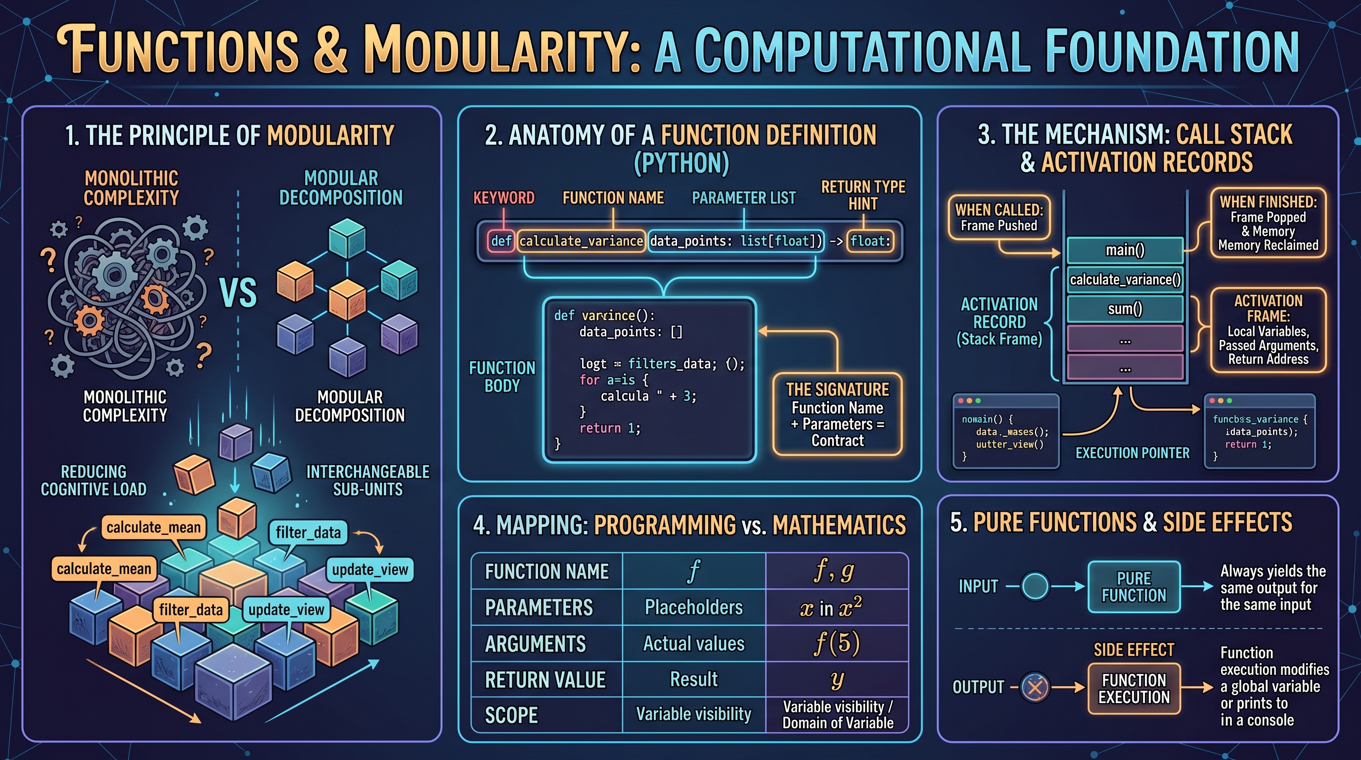
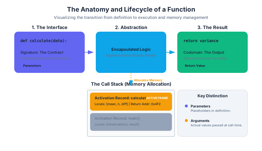
Scope and Unit Testing
Key concepts: Local scope · Global scope · Unit testing
Understanding variable visibility and ensuring individual parts of a program work correctly.
Scope and Unit Testing
In the architecture of modern software, two pillars support the structural integrity of a codebase: the management of state (Scope) and the verification of behavior (Unit Testing). While they may appear as disparate topics—one dealing with the internal visibility of variables and the other with external validation—they are deeply intertwined. A program with poorly defined scope is inherently difficult to test, and a program that is difficult to test often suffers from "leaky" scope and global state dependencies.
This article explores the mechanics of variable lifetimes, the hierarchy of lexical environments, and the rigorous methodologies used to ensure that individual components of a system function with mathematical certainty.
The Mechanics of Scope
Scope is the region of a program where a defined identifier (such as a variable or function name) is valid and accessible. From a compiler's perspective, scope defines the "lexical environment"—a mapping of names to values that changes as the program's execution pointer moves through different blocks of code.
The LEGB Rule
In languages like Python, scope resolution follows the LEGB hierarchy. When a program encounters a variable name, it searches for that name in a specific order:
- Local (L): Defined inside the current function or class method.
- Enclosing (E): Defined in the local scope of any enclosing functions (relevant in nested functions or closures).
- Global (G): Defined at the top level of the script or module.
- Built-in (B): Reserved names pre-loaded by the language (e.g.,
len,range,print).
The Principle of Least Privilege: A variable should only be visible to the components that absolutely require it. Restricting scope minimizes the "surface area" for bugs and prevents accidental state mutation.
Local vs. Global Scope
The distinction between local and global scope is primarily a matter of lifetime and visibility.
| Feature | Local Scope | Global Scope |
|---|---|---|
| Definition Location | Inside a function or block. | Outside all functions/classes. |
| Lifetime | Created on function call; destroyed on return. | Created at program start; persists until exit. |
| Accessibility | Only within the specific function. | Accessible from any function in the module. |
| Memory Management | Typically stored on the Stack. | Typically stored in Static/Data segment. |
| Risk Factor | Low; changes are isolated. | High; can lead to "spaghetti code" and side effects. |
Implementation: Scope and Closures in Python
The following implementation demonstrates the interaction between local, enclosing, and global scopes, including the use of the nonlocal and global keywords to bridge these boundaries.
# Global Scope variable
system_status = "IDLE"

def power_plant_controller(plant_id):
    """
    Demonstrates Enclosing and Local scope.
    'plant_id' is in the Local scope of power_plant_controller,
    but in the Enclosing scope of the inner 'adjust_output' function.
    """
    current_output = 0  # Local to power_plant_controller

    def adjust_output(increment):
        # Accessing Enclosing scope
        nonlocal current_output

        # Accessing Global scope
        global system_status

        if increment > 100:
            system_status = "WARNING: HIGH LOAD"

        current_output += increment
        print(f"[Plant {plant_id}] Output adjusted to {current_output}MW. Status: {system_status}")
        return current_output

    return adjust_output

# Usage
reactor_1 = power_plant_controller("RX-99")
reactor_1(50)   # Output: [Plant RX-99] Output adjusted to 50MW. Status: IDLE
reactor_1(150)  # Output: [Plant RX-99] Output adjusted to 200MW. Status: WARNING: HIGH LOAD
The Low-Level Reality: Stack Frames and Memory
To truly understand scope, one must look at how the CPU handles function calls. When a function is invoked, the system allocates a Stack Frame (or Activation Record). This frame contains the function's local variables, parameters, and the return address.
The Stack Mechanism
- Push: When
function_a()callsfunction_b(), a new frame forbis pushed onto the stack. - Isolation:
function_bcannot see the variables infunction_a's frame (unless passed as pointers/references). - Pop: When
function_bfinishes, its frame is "popped" off the stack, and its local variables are deallocated.
The following C snippet illustrates how local scope is tied to the stack pointer ($SP$).
#include <stdio.h>

void calculate_vector(int x, int y) {
    // These variables exist only while this frame is on the stack
    int magnitude_sq = (x * x) + (y * y);
    printf("Local Magnitude Squared: %d\n", magnitude_sq);
}

int main() {
    int a = 5; // Main's stack frame
    calculate_vector(a, 10);

    // magnitude_sq is unreachable here; the memory has been reclaimed.
    // printf("%d", magnitude_sq); // COMPILER ERROR: Use of undeclared identifier
    return 0;
}
Unit Testing: The Science of Verification
Unit Testing is the practice of isolating the smallest functional parts of an application (units) and verifying their correctness independently of the rest of the system. In procedural programming, a "unit" is typically a single function; in object-oriented programming, it is often a class method.
The AAA Pattern
A professional unit test follows the AAA structure to ensure clarity and repeatability:
- Arrange: Set up the necessary preconditions and inputs (e.g., initialize objects, define input variables).
- Act: Invoke the function or method being tested.
- Assert: Compare the actual result against the expected outcome.
Mathematical Definition of a Test
A unit test can be viewed as an assertion of a mapping: $$f(x) = y$$ Where $f$ is the unit under test, $x$ is the input vector, and $y$ is the expected output. A test fails if the actual output $y' \neq y$.
Designing Testable Code
The difficulty of testing is directly proportional to the complexity of a function's scope. Pure Functions—functions that depend only on their input parameters and produce no side effects—are the gold standard for testability.
Determinism and Side Effects
A function is deterministic if it always produces the same output for the same input. Functions that rely on global variables are often non-deterministic because their output can change based on the state of the global variable, which may be modified by other parts of the program.
| Function Type | Scope Dependency | Testability | Side Effects |
|---|---|---|---|
| Pure Function | Local only. | Extremely High. | None. |
| Impure Function | Local + Global. | Low (Requires setup). | Modifies external state. |
| Method (OOP) | Local + Instance (self). |
Medium (Requires object init). | Modifies object state. |
Comprehensive Testing Example: The pytest Framework
In professional Python development, pytest is the industry standard. It allows for "parameterized" testing, where a single test logic can be run against multiple sets of data.
import pytest

# The Unit Under Test
def calculate_tax(income, tax_rate):
    if income < 0:
        raise ValueError("Income cannot be negative")
    if not (0 <= tax_rate <= 1):
        raise ValueError("Tax rate must be between 0 and 1")
    return round(income * tax_rate, 2)

# The Test Suite
class TestTaxCalculations:

    def test_standard_calculation(self):
        # Arrange
        salary = 50000
        rate = 0.2
        expected = 10000.0

        # Act
        result = calculate_tax(salary, rate)

        # Assert
        assert result == expected

    @pytest.mark.parametrize("income, rate, expected", [
        (1000, 0.1, 100.0),
        (0, 0.5, 0.0),
        (100.55, 0.1, 10.06), # Testing rounding
    ])
    def test_various_inputs(self, income, rate, expected):
        assert calculate_tax(income, rate) == expected

    def test_negative_income_error(self):
        with pytest.raises(ValueError, match="Income cannot be negative"):
            calculate_tax(-100, 0.2)
Common Pitfalls in Scope and Testing
1. The "Global" Trap
Beginners often use global variables to pass information between functions. This creates a "hidden dependency." If Function A and Function B both modify Global X, testing Function A in isolation becomes impossible because its behavior depends on whether Function B ran first.
2. Shadowing
Shadowing occurs when a variable in a local scope has the same name as a variable in an outer scope. This can lead to logic errors where the programmer intends to update a global value but instead creates a new local variable.
count = 0

def increment():
    count = count + 1 # UnboundLocalError: local variable 'count' referenced before assignment
    # In Python, assigning to a variable inside a function makes it local by default.
3. Fragile Tests
A test is "fragile" if it breaks due to changes in implementation details rather than changes in behavior. Effective unit tests should treat the unit as a Black Box—focusing on inputs and outputs rather than how the calculation is performed internally.
4. High Cyclomatic Complexity
Cyclomatic Complexity measures the number of linearly independent paths through a program's source code. A function with many nested if statements and loops has high complexity and requires more unit tests to achieve full Code Coverage.
| Complexity Score | Risk | Testability |
|---|---|---|
| 1-10 | Simple, low risk. | Easy to test. |
| 11-20 | Moderate risk. | Requires significant testing. |
| 21-50 | High risk. | Difficult to test; refactor recommended. |
| >50 | Untestable. | High probability of latent bugs. |
Advanced Concept: Mocking and Dependency Injection
When a unit depends on an external system (like a database or an API), unit testing becomes difficult because the test would require that external system to be active. To solve this, engineers use Mocking.
A Mock is a simulated object that mimics the behavior of a real component in controlled ways. This ensures that the unit test is only testing the logic of the function itself, not the reliability of the internet or the database server.
# Example of running tests with coverage reporting in a real-world CI/CD pipeline
pip install pytest pytest-cov

# Run tests and generate a report showing which lines of code were NOT executed
pytest --cov=my_application --cov-report=term-missing
Summary of Best Practices
- Minimize Global State: Pass variables as arguments and return values.
- Use Descriptive Naming: Avoid name collisions to prevent accidental shadowing.
- Test Early, Test Often: Follow the "Red-Green-Refactor" cycle (Write a failing test, make it pass, then clean up the code).
- Aim for High Coverage: Ensure that your tests exercise both the "Happy Path" (valid inputs) and "Edge Cases" (invalid or extreme inputs).
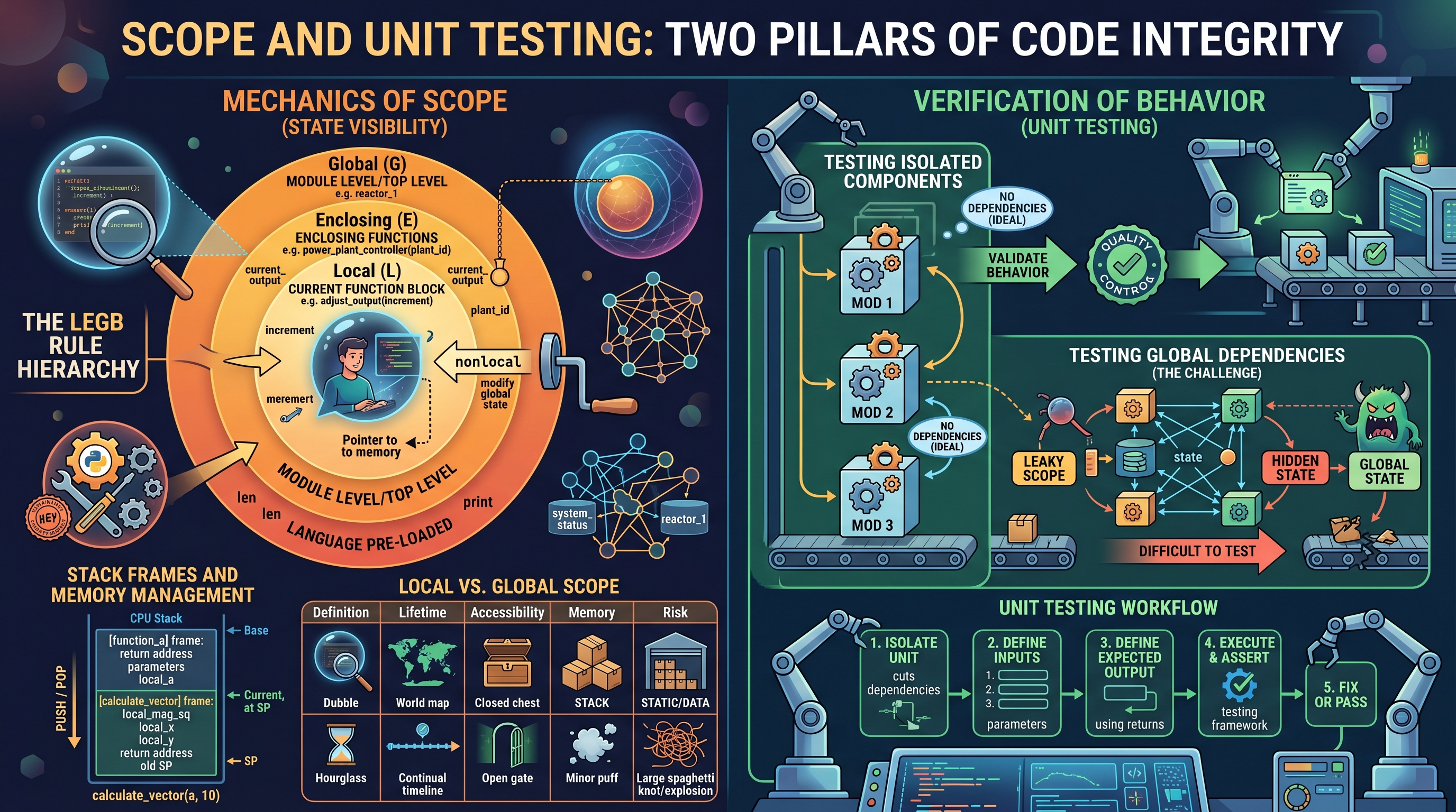
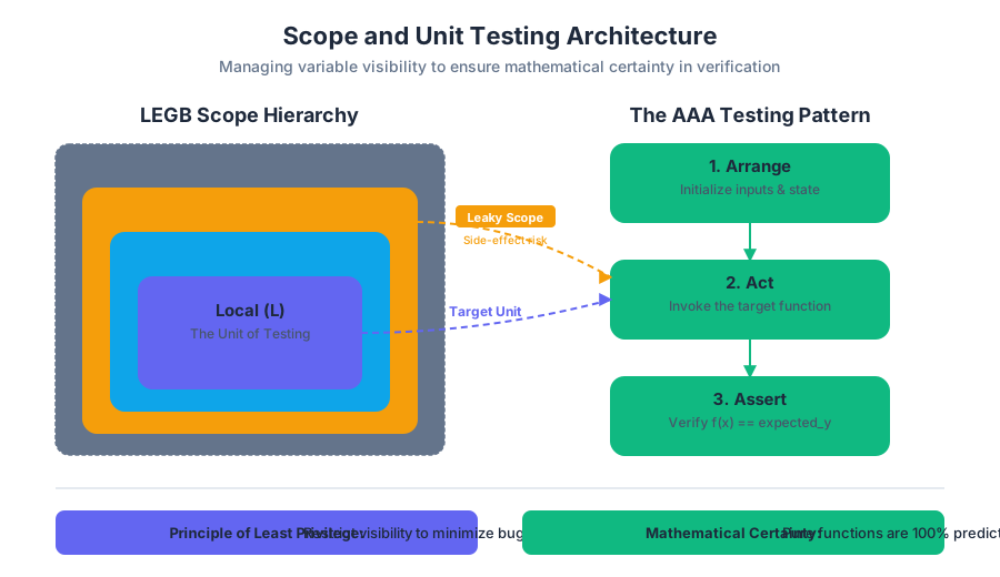
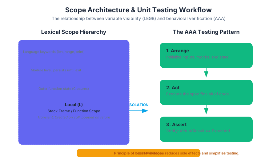
Lists and Data Processing
Key concepts: List indexing · Mutation (append, insert) · Zero-based counting
Using lists to store collections of data and learning how to manipulate them.
Lists and Data Processing
In the hierarchy of data structures, the List (or dynamic array) stands as the most fundamental tool for managing linear collections of information. While a single variable can hold a temperature reading or a user’s name, a list allows a program to process a sequence of such values, enabling the transition from simple logic to complex data processing.
At its core, a list is an ordered, mutable collection. "Ordered" implies that the position of each element is significant and preserved; "mutable" means the collection can be altered after its creation—elements can be added, removed, or swapped in place. This section explores the mechanics of how lists are indexed, how they are transformed through mutation, and how they serve as the engine for the Accumulator Pattern in modern software engineering.
The Logic of Zero-Based Counting
To the uninitiated, starting a count at zero seems counter-intuitive. However, in computer science, Zero-based Indexing is not an arbitrary choice; it is a mathematical necessity derived from how memory is addressed.
Definition: Zero-based Indexing A way of numbering the items in a list where the first item is assigned the index 0, the second item index 1, and so on. For a list of length $n$, the valid indices range from $0$ to $n-1$.
The Memory Offset Derivation
Consider a list stored in a computer's RAM. The list has a Base Address ($B$), which is the memory location of the very first element. Each element in the list occupies a fixed amount of space, let's call it the Size ($S$).
To find the memory address of the $i$-th element, the computer uses the following formula: $$\text{Address}(i) = B + (i \times S)$$
If we used 1-based indexing (where the first element is index 1), the formula would become: $$\text{Address}(i) = B + ((i - 1) \times S)$$
By starting at 0, we eliminate the subtraction operation $(i - 1)$ for every single memory access. In high-performance systems processing billions of data points, saving one subtraction per access results in significant computational efficiency.
Dijkstra’s Argument for $[a, b)$
The legendary computer scientist Edsger W. Dijkstra argued that the most elegant way to represent a range of natural numbers is using a "half-open interval" $[a, b)$, where the lower bound is included and the upper bound is excluded.
- The number of elements in the range is simply $b - a$.
- If we start at 0 and want $n$ elements, the range is $[0, n)$.
- This prevents "off-by-one" errors that frequently plague 1-based systems.
List Indexing and Access Patterns
Accessing an element in a list is an $O(1)$ operation, meaning it takes the same amount of time regardless of whether the list has ten items or ten million. This is because the memory address calculation described above is instantaneous.
Positive and Negative Indexing
Python and several other modern languages support Negative Indexing, which allows developers to reference elements relative to the end of the list.
| Index Type | Formula / Logic | Use Case |
|---|---|---|
| Positive | list[i] |
Accessing known positions from the start. |
| Negative | list[-i] maps to list[len(list) - i] |
Accessing the "last" or "second to last" items without knowing the total length. |
| Slicing | list[start:stop:step] |
Extracting sub-sections of data for batch processing. |
Slicing Mechanics
Slicing creates a new list containing a subset of the original. The syntax list[start:stop] includes the start index but excludes the stop index (following Dijkstra's $[a, b)$ principle).
# Advanced List Access and Slicing in Python
data_stream = [10.2, 15.5, 12.1, 18.9, 20.3, 14.7, 11.8]

# Accessing the tail of the data
last_three = data_stream[-3:]  # [20.3, 14.7, 11.8]

# Strided sampling (every 2nd element)
sampled_data = data_stream[::2] # [10.2, 12.1, 20.3, 11.8]

# Reversing a list via slicing
reversed_stream = data_stream[::-1]

print(f"Original: {data_stream}")
print(f"Sampled: {sampled_data}")
Mutation: The Dynamics of Change
Unlike strings (which are immutable), lists are mutable. This means we can modify the contents of a list without creating a whole new copy in memory. This is critical for "In-place" algorithms and memory efficiency.
Primary Mutation Methods
There are three main ways to mutate a list's structure:
- Append: Adding an element to the end.
- Insert: Adding an element at a specific index, shifting all subsequent elements to the right.
- Removal/Pop: Deleting an element by value or position.
| Method | Syntax | Time Complexity | Description |
|---|---|---|---|
.append(x) |
L.append(5) |
$O(1)$* | Adds x to the end. Highly efficient. |
.insert(i, x) |
L.insert(0, "A") |
$O(n)$ | Adds x at index i. Requires shifting all items after i. |
.extend(iterable) |
L.extend([1, 2]) |
$O(k)$ | Appends all elements from another collection. |
.pop(i) |
L.pop(0) |
$O(n)$ | Removes and returns item at index i. |
L[i] = x |
L[2] = 99 |
$O(1)$ | Direct replacement of an element at a known index. |
The Cost of Insertion While
.append()is usually "free" (constant time),.insert(0, x)is expensive. To put something at the beginning of a list, the computer must move every other item one slot to the right to make room. In a list of 1 million items, an insertion at the start requires 1 million move operations.
Low-Level Representation
In languages like C, a list (array) is a fixed-size block of memory. To "mutate" its size, we must manually allocate a new, larger block and copy the data. Python automates this using a Dynamic Array strategy: it allocates more space than it currently needs (over-allocation). When the "extra" space runs out, it performs a "Resize" operation.
// A low-level look at how indexing works via pointer arithmetic
#include <stdio.h>

int main() {
    int scores[5] = {88, 92, 79, 85, 90};

    // Standard access
    printf("Index 2: %d\n", scores[2]);

    // Pointer arithmetic (The "Under the Hood" reality)
    // *(base_address + offset)
    int *base_ptr = scores;
    printf("Memory Address Access: %d\n", *(base_ptr + 2));

    return 0;
}
Iteration and the Accumulator Pattern
Data processing is rarely about a single element; it is about transforming the entire collection. The most common pattern for this is the Accumulator Pattern.
The Pattern Structure
- Initialize an accumulator variable (e.g.,
total = 0orresults = []). - Iterate through the list using a loop.
- Update the accumulator inside the loop based on some logic.
- Return/Use the final accumulated value.
Worked Example: Filtering and Transforming
Suppose we have a list of sensor readings in Celsius, and we need to filter out errors (readings below -50) and convert the rest to Fahrenheit.
# The Accumulator Pattern in Action
raw_readings = [22.5, -999, 23.1, 19.8, -999, 25.0]
valid_fahrenheit = [] # 1. Initialize

for temp in raw_readings: # 2. Iterate
    if temp > -50:        # Logic: Filter errors
        f = (temp * 9/5) + 32
        valid_fahrenheit.append(f) # 3. Update

print(valid_fahrenheit) # 4. Use result
Strings vs. Lists: The Immutability Divide
While strings and lists both behave like sequences (you can index them, slice them, and loop over them), they differ in one fundamental way: Immutability.
| Feature | Lists | Strings |
|---|---|---|
| Type | Mutable | Immutable |
| Modification | L[0] = 'z' (Allowed) |
S[0] = 'z' (TypeError) |
| Memory | Modified in place | New string created for every change |
| Common Use | Collections of heterogeneous data | Textual data |
String Manipulation via Lists
Because strings are immutable, performing many small changes (like building a sentence word by word) is inefficient. Every time you add a character, a new string is created. The "Pro" way to handle this is to collect characters in a List and then use the .join() method.
# Real-world usage: Processing a list of files in a directory
# We use a shell loop to 'accumulate' filenames into a processing pipeline

files=$(ls *.txt)

for file in $files; do
    echo "Processing $file..."
    # Imagine a complex transformation here
    cat "$file" | tr '[:lower:]' '[:upper:]' > "PROCESSED_$file"
done

echo "Batch processing complete."
Common Pitfalls in List Processing
1. The "Mutation During Iteration" Trap
One of the most common logic errors occurs when a developer tries to remove items from a list while looping through it.
The Bug: When you remove the item at index
i, all subsequent items shift to indexi-1. The loop then moves to indexi+1, effectively skipping the item that just moved into indexi.
Solution: Iterate over a copy of the list (for item in my_list[:]) or use a list comprehension to create a new, filtered list.
2. Shallow vs. Deep Copies
When you write list_b = list_a, you are not creating a new list. You are creating a new "reference" to the same list in memory. Changing list_b will change list_a. To create a truly independent copy, use list_b = list_a.copy().
3. Off-by-One Errors
Because lists are zero-indexed, the last element is at len(list) - 1. Attempting to access list[len(list)] will trigger an IndexError. This is the most frequent runtime error for junior engineers.
Advanced Data Modeling: Nested Lists
Lists can contain other lists, creating multi-dimensional structures like grids, matrices, or tables.
| Row | Col 0 | Col 1 | Col 2 |
|---|---|---|---|
| 0 | Matrix[0][0] | Matrix[0][1] | Matrix[0][2] |
| 1 | Matrix[1][0] | Matrix[1][1] | Matrix[1][2] |
To access an element in a 2D list, you use two indices: matrix[row][column]. This is the basis for image processing (where an image is a 2D list of pixels) and game boards (like Chess or Tic-Tac-Toe).
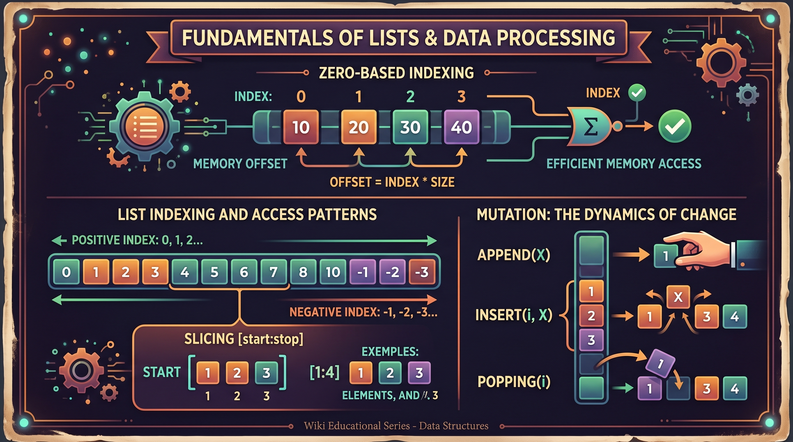
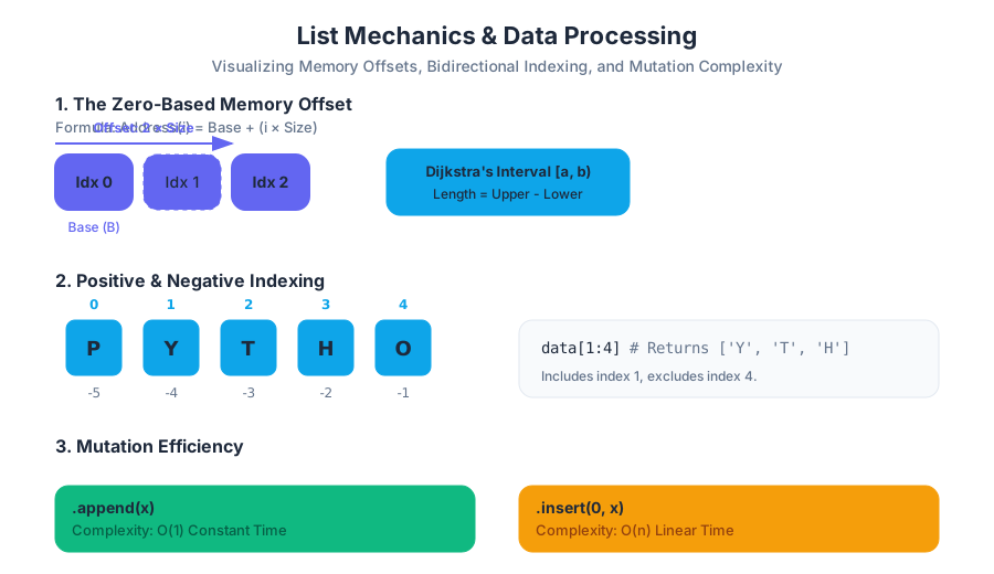
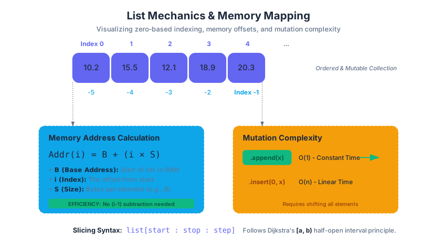
Strings and Iteration Patterns
Key concepts: String immutability · String formatting · Accumulator pattern
Manipulating text and using patterns to process sequences of data.
Strings and Iteration Patterns
In the architecture of modern software, strings are rarely just "text." They are the primary medium for data serialization (JSON, XML), the interface for human-computer interaction, and the substrate upon which most natural language processing (NLP) is built. To the uninitiated, a string is a simple sequence of characters. To the senior engineer, a string is an immutable data structure with specific memory allocation behaviors and a set of algorithmic constraints that dictate the efficiency of every iteration.
This article explores the deep mechanics of string handling, focusing on the architectural implications of immutability, the evolution of string formatting, and the ubiquitous accumulator pattern used to transform raw sequences into structured data.
String Immutability: The Architecture of Persistence
In many high-level languages—most notably Python, Java, and C#—strings are immutable. This means that once a string object is allocated in memory, its contents cannot be altered. Any operation that appears to "modify" a string actually creates an entirely new string object in a different memory location.
Why Immutability?
The design choice to make strings immutable is not arbitrary; it is a fundamental optimization for security, memory management, and concurrency:
- Thread Safety: Because strings cannot change, they are inherently thread-safe. Multiple threads can read the same string without the risk of one thread modifying the data while another is processing it, eliminating the need for complex locking mechanisms.
- String Interning: Languages can optimize memory by storing only one copy of each distinct string literal. This is known as interning. If two variables are assigned the string
"DeepWiki", they can both point to the same memory address. - Hashing Stability: Strings are frequently used as keys in hash maps (dictionaries). If a string were mutable, changing its value would change its hash code, making it impossible to retrieve the associated value from the map.
Memory Implications
When we perform a concatenation like s = s + "!", the runtime must:
- Calculate the length of the new string.
- Allocate a new block of memory sufficient for the combined length.
- Copy the characters from the old string to the new block.
- Copy the new characters to the new block.
- Update the variable
sto point to the new address.
| Property | Mutable (e.g., Lists) | Immutable (e.g., Strings) |
|---|---|---|
| In-place modification | Supported (list[0] = 'x') |
Forbidden (TypeError) |
| Memory Address | Remains constant during updates | Changes with every "modification" |
| Performance (Small updates) | $O(1)$ average | $O(n + m)$ |
| Hashability | No (cannot be dict keys) | Yes (can be dict keys) |
| Thread Safety | Requires manual locking | Inherently safe |
Low-Level Implementation: Memory Tracing
The following Python snippet demonstrates the shift in memory addresses (IDs) that occurs during "modification," proving that the original object is discarded.
# Demonstrating Immutability and Memory Allocation
def trace_string_id():
    base_str = "DeepWiki"
    original_id = id(base_str)
    print(f"Initial String: '{base_str}' | Memory Address: {original_id}")

    # Attempting to 'modify' the string
    base_str += " Article"
    new_id = id(base_str)
    print(f"Modified String: '{base_str}' | Memory Address: {new_id}")

    if original_id != new_id:
        print("Result: A new object was created. The original remains unchanged.")

    # Proof of Immutability: This will raise a TypeError
    try:
        base_str[0] = "d"
    except TypeError as e:
        print(f"Error caught: {e}")

trace_string_id()
String Formatting: The Evolution of Interpolation
String formatting is the process of building a dynamic string by injecting variables into a template. Historically, this has evolved from low-level buffer manipulation to sophisticated, type-safe interpolation.
The Three Eras of Formatting
- C-Style (% Operator): Inherited from the
printffunction in C. It uses placeholders like%sfor strings and%dfor integers. While powerful, it is error-prone regarding type matching and readability. - The
.format()Method: Introduced to provide more flexibility, allowing for positional and keyword arguments, as well as advanced alignment and padding. - F-Strings (Literal String Interpolation): The modern standard. F-strings are evaluated at runtime, allowing for embedded expressions and significantly higher performance because they are parsed into a series of constant strings and expressions rather than being processed as a template at runtime.
Comparative Performance and Syntax
| Method | Syntax Example | Pros | Cons |
|---|---|---|---|
| % Operator | "%s: %d" % (name, val) |
Familiar to C/C++ devs | Strict type requirements |
| .format() | "{}: {}".format(n, v) |
Flexible, good for templates | Verbose for simple cases |
| F-Strings | f"{name}: {val}" |
Fastest, most readable | Only available in Python 3.6+ |
| Template Strings | Template("$n").substitute(n=name) |
Secure for user-provided input | Limited features |
Systems-Level Representation: C Buffer Formatting
In lower-level languages like C, formatting requires manual buffer management, highlighting the risks of buffer overflows that modern languages handle automatically.
#include <stdio.h>
#include <string.h>

/**
 * Demonstrates the manual nature of string formatting in C.
 * Unlike Python f-strings, we must ensure the destination buffer
 * is large enough to hold the result.
 */
int main() {
    char buffer[100];
    char* title = "DeepWiki";
    int version = 2;
    float latency = 0.45;

    // snprintf is the 'safe' way to format, preventing buffer overflows
    int written = snprintf(buffer, sizeof(buffer),
                           "System: %s | V: %d | Latency: %.2fms",
                           title, version, latency);

    if (written >= sizeof(buffer)) {
        printf("Error: String truncated. Buffer too small.\n");
    } else {
        printf("Formatted Output: %s\n", buffer);
    }

    return 0;
}
The Accumulator Pattern: Building Results Iteratively
The Accumulator Pattern is a fundamental algorithmic structure where a variable (the "accumulator") is initialized before a loop and updated within the loop to build a final result. When applied to strings, this pattern is the engine behind data transformation, filtering, and custom serialization.
Mathematical Derivation of the Pattern
Let $S$ be the initial state of the accumulator. Let $I = {i_1, i_2, ..., i_n}$ be a sequence of inputs. Let $f(acc, input)$ be a transformation function.
The accumulator pattern follows the recurrence: $$acc_0 = S$$ $$acc_k = f(acc_{k-1}, i_k)$$ $$Result = acc_n$$
The Concatenation Trap
A common pitfall in the accumulator pattern is using += to build a string inside a loop. Because of immutability, each += operation creates a new string.
- First iteration: Copy 1 char.
- Second iteration: Copy 2 chars.
- $N^{th}$ iteration: Copy $N$ chars.
This results in an $O(N^2)$ time complexity, which is disastrous for large datasets. The industry-standard solution is to accumulate elements in a list (which is mutable and has $O(1)$ append time) and then use a
joinoperation to create the final string in a single $O(N)$ pass.
Real-World Usage: Log Sanitization Pipeline
In this example, we use the accumulator pattern to process a raw log file, filtering out sensitive information and building a sanitized report.
import re

def sanitize_logs(raw_logs):
    """
    Uses the Accumulator Pattern to filter PII from log sequences.
    Accumulates into a list to maintain O(n) complexity.
    """
    # 1. Initialize the accumulator
    sanitized_entries = []

    # 2. Iterate through the sequence
    for entry in raw_logs:
        # Transformation logic (f(acc, input))
        # Masking IP addresses with a regex
        clean_entry = re.sub(r'\d{1,3}\.\d{1,3}\.\d{1,3}\.\d{1,3}', '[REDACTED_IP]', entry)

        # Filtering logic
        if "DEBUG" not in clean_entry:
            # 3. Update the accumulator
            sanitized_entries.append(clean_entry)

    # 4. Finalize the result
    return "\n".join(sanitized_entries)

# Example CLI usage simulation
log_data = [
    "2023-10-01 10:00:01 INFO Connection from 192.168.1.1",
    "2023-10-01 10:00:02 DEBUG Handshake initiated",
    "2023-10-01 10:00:05 WARN Unauthorized access attempt by 10.0.0.55"
]

print(sanitize_logs(log_data))
Iteration Patterns: Beyond the Simple Loop
Iterating over strings is not limited to "for each character." Advanced patterns allow for complex parsing and data extraction.
1. Index-Based Iteration
Used when the position of the character matters (e.g., checking the character before the current one).
Theorem: For any string of length $L$, the valid index range is $[0, L-1]$. Accessing $L$ results in an
IndexError(Off-by-one error).
2. Slicing and Windowing
Slicing allows for the extraction of sub-sequences. A Sliding Window is a specific iteration pattern where we look at a fixed-size chunk of the string at each step. This is essential for tasks like finding DNA motifs or calculating rolling hashes.
| Pattern | Logic | Complexity | Use Case |
|---|---|---|---|
| Linear Scan | for char in string |
$O(N)$ | Counting characters, simple search |
| Reverse Scan | for i in range(len(s)-1, -1, -1) |
$O(N)$ | Palindrome checks, suffix parsing |
| Sliding Window | s[i : i+k] |
$O(N \cdot K)$ | Substring matching, N-grams |
| Two-Pointer | while left < right |
$O(N)$ | In-place reversals, sorting logic |
Example: The Sliding Window Pattern
This shell-style logic (using Python for clarity) demonstrates how to extract all 3-character sequences (trigrams) from a string, a common task in computational linguistics.
def get_trigrams(text):
    """
    Implements a sliding window iteration pattern.
    """
    trigrams = []
    # We stop at len - 2 to ensure the window (i, i+1, i+2) stays in bounds
    for i in range(len(text) - 2):
        window = text[i : i+3]
        trigrams.append(window)
    return trigrams

# Input: "ITERATION"
# Output: ['ITE', 'TER', 'ERA', 'RAT', 'ATI', 'TIO', 'ION']
print(f"Trigrams: {get_trigrams('ITERATION')}")
Common Pitfalls and Edge Cases
- The Off-By-One Error: When iterating by index, beginners often try to access
string[len(string)]. Remember that indexing is zero-based. - Unicode and Multi-byte Characters: In modern systems, one "character" (grapheme) might consist of multiple bytes or even multiple code points (e.g., emojis with skin tone modifiers). Simple iteration might split an emoji in half.
- Empty String Handling: Always ensure your accumulator logic handles
""gracefully. An empty string has a length of 0, and loops over it will not execute, which might leave your accumulator in an uninitialized or invalid state.
Key Insight: Always prefer
"".join(list_accumulator)overstring_accumulator += valuein performance-critical loops. The difference is the difference between linear $O(N)$ and quadratic $O(N^2)$ time.
Summary of Engineering Principles
Strings are the most common data type, but their simplicity is deceptive. By understanding that strings are immutable, we write safer, more predictable code. By mastering formatting, we create more maintainable and performant interfaces. And by applying the accumulator pattern correctly, we ensure our text-processing algorithms scale linearly with our data. Whether you are building a simple script or a massive distributed system, these patterns form the bedrock of efficient computation.
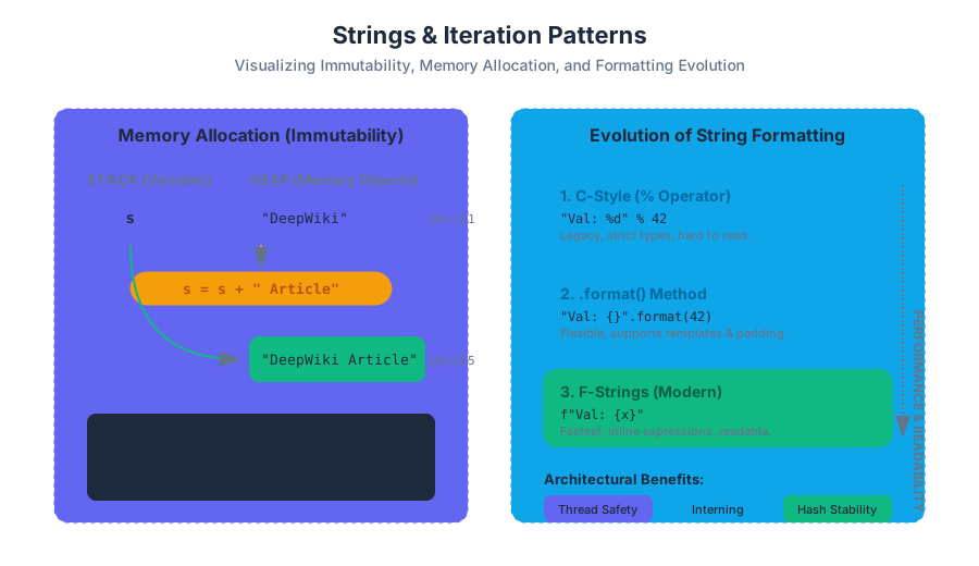
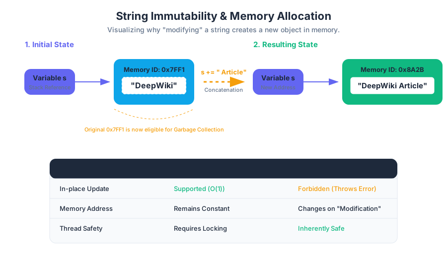
Source Materials
Study Computing with AI — Free on Lykke
Sign up for free to generate personalized flashcards, quizzes, and study guides from this course. Chat with an AI tutor that knows the material.
Get Started FreeView this course wiki on Lykke · Browse all public course wikis