College Algebra

Linear Equations and Inequalities

Linearity is the cornerstone of algebraic analysis. In its most fundamental form, a linear equation represents a relationship where the rate of change between variables is constant. This section explores the mechanics of manipulating these expressions, the logical frameworks governing inequalities, and the specialized handling required for absolute value functions. We move beyond simple one-step arithmetic into the realm of multi-step isolation, logical conjunctions, and the rigorous classification of solution sets.

Multi-Step Linear Equations

A multi-step linear equation is an equality involving one or more operations—distributive property, combining like terms, and inverse operations—required to isolate the target variable. Mathematically, any linear equation in one variable can be reduced to the standard form $ax + b = 0$, where $a \neq 0$.

The Mechanics of Isolation

The primary objective in solving linear equations is variable isolation. This is achieved through the application of the Properties of Equality, which maintain the "balance" of the equation by performing identical operations on both sides of the equal sign.

Property	Algebraic Definition	Description
Addition Property	If $a = b$, then $a + c = b + c$	Adding the same value to both sides preserves equality.
Subtraction Property	If $a = b$, then $a - c = b - c$	Subtracting the same value from both sides preserves equality.
Multiplication Property	If $a = b$, then $ac = bc$	Multiplying both sides by the same non-zero value preserves equality.
Division Property	If $a = b$ and $c \neq 0$, then $a/c = b/c$	Dividing both sides by the same non-zero value preserves equality.
Distributive Property	$a(b + c) = ab + ac$	Allows for the removal of parentheses by distributing a multiplier.

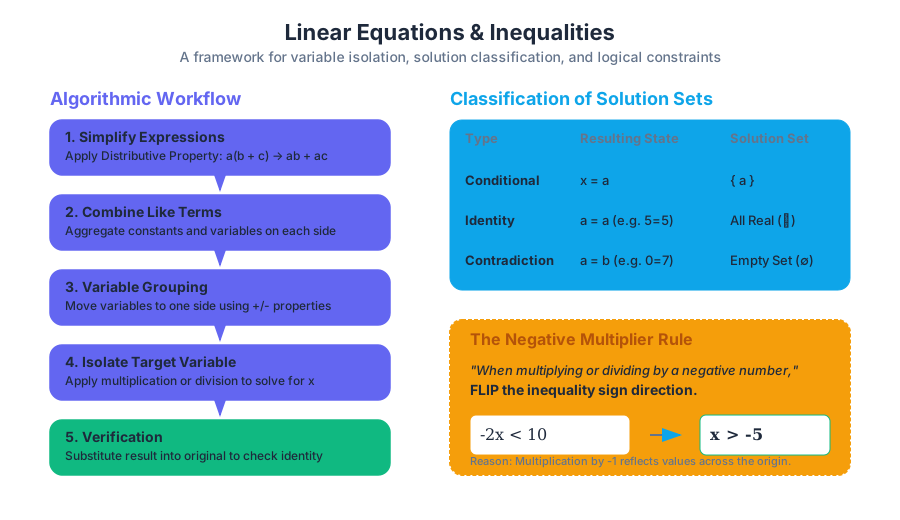
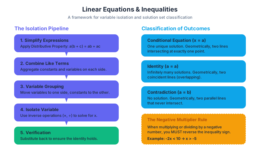
Algorithmic Workflow for Multi-Step Equations

To solve a complex equation such as $3(2x - 4) + 5 = 2x - (x + 8)$, follow a structured pipeline:

1. Simplify Expressions: Apply the distributive property to eliminate parentheses.
2. Combine Like Terms: Aggregate constants and variable terms on each individual side.
3. Variable Grouping: Use addition or subtraction to move all variable terms to one side and all constants to the other.
4. Isolate: Use multiplication or division to solve for the variable (coefficient of 1).
5. Verify: Substitute the result back into the original equation to ensure the identity holds.

# A robust symbolic solver for linear equations of the form ax + b = cx + d
# This implementation uses basic parsing logic to demonstrate the isolation algorithm.

def solve_linear(left_coeff, left_const, right_coeff, right_const):
    """
    Solves for x in: (left_coeff * x) + left_const = (right_coeff * x) + right_const
    """
    print(f"Solving: {left_coeff}x + {left_const} = {right_coeff}x + {right_const}")
    
    # Step 1: Group variables on the left (Subtract right_coeff * x from both sides)
    final_coeff = left_coeff - right_coeff
    
    # Step 2: Group constants on the right (Subtract left_const from both sides)
    final_const = right_const - left_const
    
    # Step 3: Handle solution cases
    if final_coeff == 0:
        if final_const == 0:
            return "Infinitely Many Solutions (Identity)"
        else:
            return "No Solution (Contradiction)"
    
    # Step 4: Final Division
    solution = final_const / final_coeff
    return f"x = {solution}"

# Example: 5x + 10 = 2x + 25
print(solve_linear(5, 10, 2, 25))

The Number of Solutions

Not every linear equation results in a single, discrete value for the variable. In college algebra, we categorize equations based on their solution sets. This classification is vital for understanding the geometric relationship between two lines or the consistency of a system.

Classification of Solution Sets

When simplifying a linear equation, if the variable terms cancel out (e.g., $0x$), the resulting numeric statement determines the nature of the solution.

Resulting Statement	Classification	Geometric Interpretation	Solution Set
$x = a$	Conditional	Two lines intersecting at exactly one point.	${a}$
$a = a$ (e.g., $5=5$)	Identity	Two coincident lines (one on top of the other).	All Real Numbers ($\mathbb{R}$)
$a = b$ (e.g., $0=7$)	Contradiction	Two parallel lines that never intersect.	Empty Set ($\emptyset$)

Theorem of Linear Consistency: A linear equation in the form $ax + b = cx + d$ has exactly one solution if and only if $a \neq c$. If $a = c$, the equation is either an identity (if $b = d$) or a contradiction (if $b \neq d$).

Linear Inequalities and Interval Notation

Linear inequalities extend the concept of equations to relationships of "greater than" or "less than." Unlike equations, which typically yield points, inequalities yield regions or intervals.

The Negative Multiplier Rule

The most critical distinction in solving inequalities is the behavior of the inequality sign during multiplication or division by a negative number.

Key Rule: When multiplying or dividing both sides of an inequality by a negative number, the direction of the inequality symbol must be reversed.

This is because multiplying by a negative number reflects the values across the origin on a number line, effectively reversing their relative order.

Representing Solutions

Solutions to inequalities are represented in three primary ways:

1. Inequality Notation: $x > 5$
2. Set-Builder Notation: ${x \mid x > 5}$
3. Interval Notation: $(5, \infty)$

Symbol	Meaning	Circle on Graph	Bracket/Parenthesis
$<$	Less than	Open	$($ or $)$
$>$	Greater than	Open	$($ or $)$
$\leq$	Less than or equal to	Closed	$[$ or $]$
$\geq$	Greater than or equal to	Closed	$[$ or $]$

Compound Inequalities

A compound inequality consists of two separate inequalities joined by the logical operators AND or OR. These represent the intersection and union of sets, respectively.

Conjunctions (AND)

A conjunction is true only if both inequalities are satisfied. This usually represents a bounded interval.

• Notation: $x > a$ AND $x < b$, often written as $a < x < b$.
• Set Theory: $A \cap B$ (Intersection).
• Visual: The "middle" section where two shaded regions overlap.

Disjunctions (OR)

A disjunction is true if at least one of the inequalities is satisfied. This usually represents two divergent intervals.

• Notation: $x < a$ OR $x > b$.
• Set Theory: $A \cup B$ (Union).
• Visual: Two separate shaded regions pointing away from each other.

\text{Example of a Conjunction derivation:} \\
-5 \leq 2x + 3 < 11 \\
\text{Step 1: Subtract 3 from all parts} \\
-8 \leq 2x < 8 \\
\text{Step 2: Divide all parts by 2} \\
-4 \leq x < 4 \\
\text{Interval Notation: } [-4, 4)

Absolute Value Equations

The absolute value of a number, denoted $|x|$, is defined as its distance from zero on the number line. Because distance is non-negative, the output of an absolute value function is always $\geq 0$.

Solving $|ax + b| = c$

To solve an absolute value equation, you must account for the two possible scenarios that result in the same distance:

1. The expression inside the bars is positive: $ax + b = c$
2. The expression inside the bars is negative: $ax + b = -c$

Important Pitfall: Before branching into two equations, you must isolate the absolute value expression. If you are left with $|ax + b| = -c$ (where $c$ is positive), there is no solution, as an absolute value cannot equal a negative distance.

Equation Type	Branch 1	Branch 2	Condition
$	x	= k$	$x = k$
$	x	< k$	$x < k$
$	x	> k$	$x > k$

Absolute Value Inequalities: "Great-OR" and "Less-THEN"

A helpful mnemonic for remembering how to branch inequalities:

• $|x| > k$ is a Great-OR problem (uses the OR operator).
• $|x| < k$ is a Less-THEN (Less-Than) problem (uses the AND operator).

/**
 * Real-world usage: A validation utility to check if a 
 * measurement falls within a specific tolerance using 
 * absolute value logic.
 */

interface ToleranceCheck {
    value: number;
    target: number;
    tolerance: number;
}

function isWithinTolerance(params: ToleranceCheck): boolean {
    const { value, target, tolerance } = params;
    
    // Mathematically: |value - target| <= tolerance
    const deviation = Math.abs(value - target);
    
    console.log(`Checking value: ${value} against target: ${target}`);
    console.log(`Absolute deviation: ${deviation}`);
    
    return deviation <= tolerance;
}

const sensorData = { value: 98.6, target: 100, tolerance: 2.0 };
const result = isWithinTolerance(sensorData);
console.log(`Is within tolerance: ${result}`); // true, because 1.4 <= 2.0

Interpreting Equations in Context

In applied mathematics, linear equations and inequalities serve as models for constraints and relationships.

Modeling with Two Variables

When dealing with two-variable equations (e.g., $Ax + By = C$), we often interpret the intercepts:

• X-intercept: The value of $x$ when $y=0$. In a business context, this might represent the maximum number of units produced if no resources are allocated to the second product.
• Y-intercept: The value of $y$ when $x=0$.
• Slope ($m$): The rate of change. If $y$ is cost and $x$ is time, the slope is the cost per unit of time.

Systems in Context

Solving a system of linear equations (finding where two lines meet) allows us to find break-even points or equilibrium.

• If the system has one solution, the lines intersect (different slopes).
• If the system has no solution, the constraints are mutually exclusive (parallel lines).
• If the system has infinite solutions, the two constraints are redundant (the same line).

# A simple CLI workflow using 'bc' (arbitrary precision calculator) 
# to solve a linear growth problem: 
# "If a plant starts at 5cm and grows 2cm/week, when will it reach 25cm?"
# Equation: 2x + 5 = 25

TARGET=25
START=5
RATE=2

# Step 1: Subtract start from target
REMAINING_GROWTH=$(echo "$TARGET - $START" | bc)

# Step 2: Divide by rate
WEEKS=$(echo "scale=2; $REMAINING_GROWTH / $RATE" | bc)

echo "The plant will reach $TARGET cm in $WEEKS weeks."

Common Pitfalls and Edge Cases

1. Distributing Negatives: A common error is failing to distribute a negative sign to all terms inside a parenthesis. For example, $-(x - 5)$ becomes $-x + 5$, not $-x - 5$.
2. Dividing by Zero: In literal equations (equations with multiple variables), one must state constraints. If solving $ax = b$ for $x$, you must specify $a \neq 0$.
3. Absolute Value Logic: Forgetting to isolate the absolute value before branching. In $2|x| + 4 = 10$, you must subtract 4 and divide by 2 before setting up $x = 3$ and $x = -3$.
4. Inequality Direction: Forgetting to flip the sign when multiplying by $-1$. This is the most frequent error in linear inequality problems.
5. Empty Sets in Absolute Value: $|x + 5| = -2$ has no solution. Distance cannot be negative. Students often robotically solve $x+5 = -2$ and $x+5 = 2$, obtaining extraneous solutions.

Linear Forms and Coordinate Geometry

The study of linear forms is the foundational bridge between pure algebra and geometric intuition. In the Cartesian plane, a line is more than a sequence of points; it is the visual manifestation of a constant rate of change. Whether we are modeling the trajectory of a particle in a physics engine or calculating the depreciation of an asset in a financial model, the ability to manipulate and interpret linear equations is a prerequisite for all higher-level mathematics, including Calculus and Linear Algebra.

The Fundamental Constant: Slope ($m$)

At the heart of every linear form lies the concept of slope, often denoted by the variable $m$. Mathematically, the slope represents the ratio of the vertical change (the "rise") to the horizontal change (the "run") between any two distinct points on a line.

Definition: The Slope Formula For any two points $(x_1, y_1)$ and $(x_2, y_2)$ where $x_1 \neq x_2$, the slope $m$ is defined as: $$m = \frac{\Delta y}{\Delta x} = \frac{y_2 - y_1}{x_2 - x_1}$$

Why the Slope Matters

In a physical context, the slope is the rate of change. If the x-axis represents time and the y-axis represents distance, the slope is velocity. If the x-axis is production volume and the y-axis is cost, the slope is the marginal cost per unit. Understanding the slope allows us to predict future states based on current trajectories.

Classification of Slopes

The value of $m$ dictates the orientation and behavior of the line within the coordinate system.

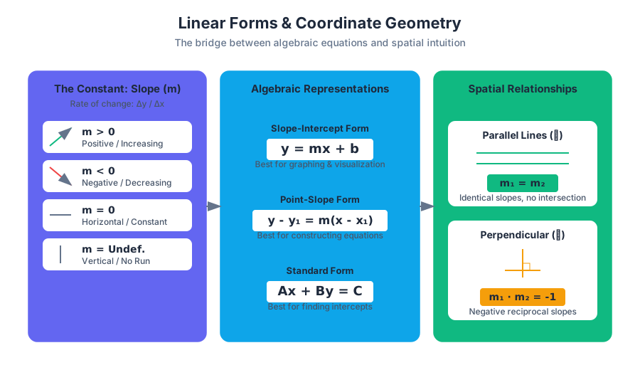
Slope Value ($m$)	Direction	Geometric Interpretation
$m > 0$	Upward (Left to Right)	Positive correlation; as $x$ increases, $y$ increases.
$m < 0$	Downward (Left to Right)	Negative correlation; as $x$ increases, $y$ decreases.
$m = 0$	Horizontal	No change in $y$; the line is parallel to the x-axis.
$m$ is Undefined	Vertical	No change in $x$; the line is parallel to the y-axis.

Slope-Intercept Form: The Visual Standard

The most common way to express a linear equation is the Slope-Intercept Form. It is prized for its readability and the ease with which it can be graphed.

The Formula

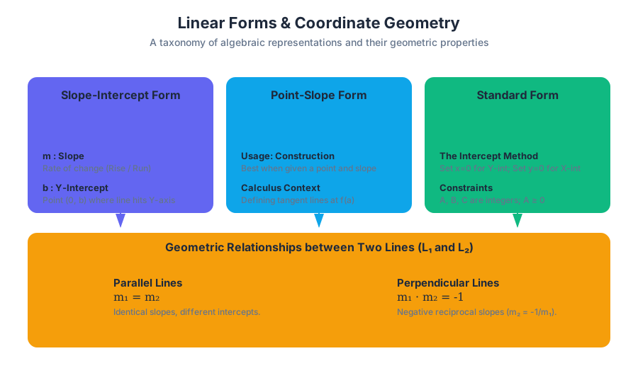
The slope-intercept form is written as: $$y = mx + b$$ Where:

• $m$ is the slope.
• $b$ is the y-intercept, the point $(0, b)$ where the line crosses the vertical axis.

Implementation in Software

In computational geometry or data science, we often need to represent these lines programmatically to calculate intersections or trendlines.

class LinearEquation:
    """
    Represents a linear equation in the form y = mx + b.
    Provides methods for coordinate calculation and form conversion.
    """
    def __init__(self, m: float, b: float):
        self.m = m  # Slope
        self.b = b  # Y-intercept

    def calculate_y(self, x: float) -> float:
        """Returns the y-value for a given x."""
        return (self.m * x) + self.b

    def calculate_x(self, y: float) -> float:
        """Returns the x-value for a given y. Raises error if horizontal."""
        if self.m == 0:
            raise ValueError("Horizontal lines do not have a unique x for a given y.")
        return (y - self.b) / self.m

    def __repr__(self):
        sign = "+" if self.b >= 0 else "-"
        return f"y = {self.m}x {sign} {abs(self.b)}"

# Example Usage:
line = LinearEquation(m=2.5, b=-10)
print(f"At x=4, y is: {line.calculate_y(4)}") # Output: 0.0

Point-Slope Form: The Engineer’s Tool

While slope-intercept is great for reading a graph, Point-Slope Form is the superior tool for constructing an equation when you are given a specific point and a known rate of change.

The Derivation

The point-slope form is derived directly from the definition of slope. If we know a fixed point $(x_1, y_1)$ and a general point $(x, y)$, the slope $m$ is: $$m = \frac{y - y_1}{x - x_1}$$ By multiplying both sides by $(x - x_1)$, we arrive at the standard point-slope equation: $$y - y_1 = m(x - x_1)$$

When to Use Point-Slope

1. Given a point and a slope: Immediate substitution.
2. Given two points: Calculate $m$ first, then use either point in this form.
3. Calculus: When finding the equation of a tangent line to a curve at a specific point $(a, f(a))$, the point-slope form is the natural choice: $y - f(a) = f'(a)(x - a)$.

Standard Form and Intercepts

The Standard Form of a linear equation is expressed as: $$Ax + By = C$$ Where $A, B,$ and $C$ are typically integers, and $A$ is non-negative.

The Power of Intercepts

Standard form is particularly useful for finding the intercepts—the points where the line crosses the axes. This "Intercept Method" is often the fastest way to sketch a line by hand.

Intercept Type	Definition	How to Solve
x-intercept	Where the line hits the x-axis ($y=0$)	Set $y=0$, solve $Ax = C \rightarrow x = C/A$
y-intercept	Where the line hits the y-axis ($x=0$)	Set $x=0$, solve $By = C \rightarrow y = C/B$

Mathematical Derivation: Perpendicular Slopes

A common question in coordinate geometry is why perpendicular lines have negative reciprocal slopes. We can prove this using geometric rotation or vectors.

Let Line 1 have slope m1 = tan(θ).
A line perpendicular to it (Line 2) is rotated by 90 degrees (π/2 radians).
The slope of Line 2 is m2 = tan(θ + π/2).

Using the trigonometric identity:
tan(θ + π/2) = -cot(θ) = -1/tan(θ)

Therefore:
m2 = -1 / m1
Or:
m1 * m2 = -1

Geometric Relationships: Parallel and Perpendicular

The relationship between two lines is determined entirely by their slopes. This is a critical concept in spatial partitioning and collision detection in computer graphics.

Parallel Lines

Two lines are parallel if they lie in the same plane and never intersect.

• Condition: $m_1 = m_2$ and $b_1 \neq b_2$.
• If the y-intercepts are also the same, the lines are coincident (they are the same line).

Perpendicular Lines

Two lines are perpendicular if they intersect at a right angle ($90^\circ$).

• Condition: $m_1 \cdot m_2 = -1$.
• Alternatively: $m_2 = -\frac{1}{m_1}$.

Summary of Relationships

Relationship	Slopes ($m_1, m_2$)	Visual Result
Parallel	$m_1 = m_2$	Lines run side-by-side, never touching.
Perpendicular	$m_1 = -1/m_2$	Lines cross at exactly 90 degrees.
Intersecting	$m_1 \neq m_2$	Lines cross at exactly one point.
Coincident	$m_1 = m_2, b_1 = b_2$	The equations describe the same line.

Special Cases: Vertical and Horizontal Lines

Vertical and horizontal lines are the "edge cases" of linear geometry. They often break standard algorithms because they involve zero or undefined values.

Horizontal Lines

• Equation: $y = k$ (where $k$ is a constant).
• Slope: $0$.
• Behavior: For every value of $x$, $y$ remains the same. It is parallel to the x-axis.

Vertical Lines

• Equation: $x = h$ (where $h$ is a constant).
• Slope: Undefined (division by zero in the slope formula).
• Behavior: It is not a function (it fails the vertical line test). It is parallel to the y-axis.

Real-World Application: Linear Regression and Data Trends

In modern data science, we rarely have points that fit perfectly on a line. Instead, we use the Method of Least Squares to find the "Line of Best Fit." While the underlying data is messy, the output is a simple linear form: $y = mx + b$.

Usage Example: SQL Trend Analysis

If we store time-series data in a database, we can use linear forms to project future values.

-- Calculating the components for a simple linear regression
-- to find the slope (m) of sales over time.
SELECT
    count(*) AS n,
    sum(x) AS sum_x,
    sum(y) AS sum_y,
    sum(x*y) AS sum_xy,
    sum(x*x) AS sum_xx,
    -- The formula for slope m:
    ((count(*) * sum(x*y)) - (sum(x) * sum(y))) / 
    ((count(*) * sum(x*x)) - (sum(x) * sum(x))) AS slope_m
FROM sales_data;

Common Pitfalls and Misconceptions

1. The "Zero vs. Undefined" Confusion: A horizontal line has a slope of $0$. A vertical line has an undefined slope. These are not interchangeable. In programming, a vertical line will often trigger a DivideByZero exception.
2. Negative Reciprocal Errors: When finding a perpendicular slope, students often forget one of the two steps. You must both flip the fraction and change the sign.
   • Correct: If $m = 2/3$, perpendicular $m = -3/2$.
   • Incorrect: If $m = 2/3$, perpendicular $m = 3/2$ (forgot sign) or $m = -2/3$ (forgot flip).
3. Intercept Misplacement: The y-intercept is the point $(0, b)$, not $(b, 0)$. The latter is the x-intercept.

Advanced Concept: Distance from a Point to a Line

In coordinate geometry, we often need to find the shortest distance between a point $(x_0, y_0)$ and a line defined by $Ax + By + C = 0$. This distance $d$ is the length of the perpendicular segment from the point to the line.

Theorem: Point-to-Line Distance The distance $d$ is given by: $$d = \frac{|Ax_0 + By_0 + C|}{\sqrt{A^2 + B^2}}$$

This formula is used extensively in machine learning (Support Vector Machines) to determine the "margin" between different classes of data points.

Worked Example

Find the distance between the point (2, 3) and the line $3x - 4y + 1 = 0$.

1. Identify constants: $A=3, B=-4, C=1$.
2. Identify point: $x_0=2, y_0=3$.
3. Substitute into formula: $$d = \frac{|3(2) + (-4)(3) + 1|}{\sqrt{3^2 + (-4)^2}}$$ $$d = \frac{|6 - 12 + 1|}{\sqrt{9 + 16}}$$ $$d = \frac{|-5|}{5} = 1$$ The point is exactly 1 unit away from the line.

Visualizing Linear Systems in Web Applications

For developers building interactive dashboards, rendering these lines requires translating Cartesian coordinates to screen coordinates (where the y-axis is often inverted).

/**
 * Renders a linear equation onto an HTML5 Canvas.
 * Translates Cartesian (0,0 at center) to Screen (0,0 at top-left).
 */
function drawLine(ctx, m, b, width, height) {
    const centerX = width / 2;
    const centerY = height / 2;
    const scale = 20; // Pixels per unit

    ctx.beginPath();
    ctx.strokeStyle = '#007bff';
    ctx.lineWidth = 2;

    for (let screenX = 0; screenX < width; screenX++) {
        // Convert screen X to Cartesian X
        let x = (screenX - centerX) / scale;
        
        // Calculate Cartesian Y
        let y = m * x + b;
        
        // Convert Cartesian Y to screen Y (invert Y)
        let screenY = centerY - (y * scale);
        
        if (screenX === 0) {
            ctx.moveTo(screenX, screenY);
        } else {
            ctx.lineTo(screenX, screenY);
        }
    }
    ctx.stroke();
}

• Slope ($m$): The ratio of vertical change to horizontal change ($\Delta y / \Delta x$).
• Y-intercept ($b$): The y-coordinate where a line crosses the y-axis (where $x=0$).
• Slope-Intercept Form: $y = mx + b$; most useful for graphing and identifying rate of change.
• Point-Slope Form: $y - y_1 = m(x - x_1)$; most useful for creating an equation given a point and slope.
• Standard Form: $Ax + By = C$; useful for finding intercepts and solving systems of equations.
• Parallel Lines: Lines with identical slopes ($m_1 = m_2$) that never intersect.
• Perpendicular Lines: Lines whose slopes are negative reciprocals ($m_1 \cdot m_2 = -1$), meeting at a $90^\circ$ angle.
• Undefined Slope: The slope of a vertical line, where the change in $x$ is zero.

1. What is the slope of a line perpendicular to $y = -4x + 7$?
   • A) -4
   • B) 4
   • C) 1/4 (Correct)
   • D) -1/4
2. Which form is most efficient for finding the x and y intercepts of a line?
   • A) Slope-intercept form
   • B) Point-slope form
   • C) Standard form (Correct)
   • D) Quadratic form
3. If a line has a slope of 0, what is its geometric orientation?
   • A) Vertical
   • B) Horizontal (Correct)
   • C) Diagonal
   • D) It is a single point
4. Calculate the slope between points (2, 5) and (4, 11).
   • A) 2
   • B) 3 (Correct: (11-5)/(4-2) = 6/2 = 3)
   • C) 6
   • D) 1/3
5. True or False: A vertical line is a function.
   • A) True
   • B) False (Correct: It fails the vertical line test)
6. What is the y-intercept of the line $3x + 2y = 12$?
   • A) 4
   • B) 6 (Correct: Set x=0, 2y=12, y=6)
   • C) 12
   • D) 3

Core Objectives

• Master Slope Calculation: Be able to find $m$ from two points, a graph, or an equation.
• Form Conversion: Practice converting between Standard, Point-Slope, and Slope-Intercept forms.
• Geometric Logic: Immediately identify if lines are parallel or perpendicular by looking at their $m$ values.
• Graphing Proficiency: Use the intercept method for Standard form and the "start at $b$, move by $m$" method for Slope-Intercept form.

Practice Exercises

1. Write the equation of a line passing through (1, 2) and parallel to $y = 3x - 5$.
2. Convert $y - 4 = -2(x + 3)$ into Standard Form.
3. Find the distance from the origin (0,0) to the line $y = x + 2$.
4. Determine the equation of the vertical line passing through (-7, 12).

Introduction to Functions

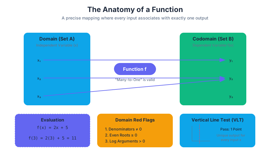
In the architecture of mathematics, a function is the fundamental unit of mapping. It represents a precise relationship where every valid input is associated with exactly one output. While elementary algebra often treats functions as mere "equations," a rigorous approach views them as transformations between sets—a concept that underpins everything from signal processing in electrical engineering to the logic gates in a microprocessor.

The Formal Definition of a Function

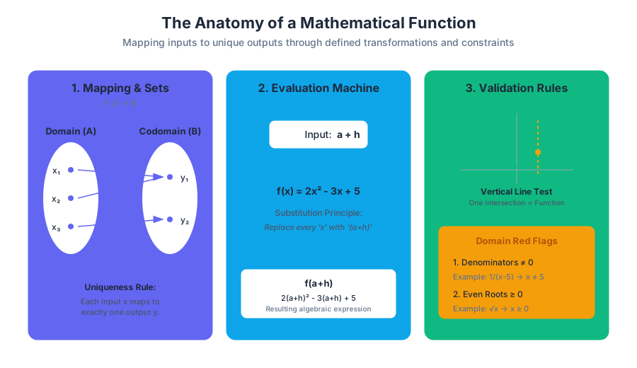
At its most abstract, a function $f$ from a set $A$ (the domain) to a set $B$ (the codomain) is a relation that associates each element $x \in A$ with exactly one element $y \in B$. We denote this as $f: A \to B$.

The Uniqueness Requirement: For a relation to be a function, it must satisfy the condition that if $(x, y) \in f$ and $(x, z) \in f$, then $y = z$. In simpler terms, a single input cannot produce two different outputs.

Distinguishing Relations from Functions

All functions are relations, but not all relations are functions. A relation is simply any set of ordered pairs. To determine if a relation is a function, we apply the Vertical Line Test (VLT) to its graph: if any vertical line intersects the graph at more than one point, the relation fails to be a function because a single $x$-value maps to multiple $y$-values.

Feature	Relation	Function
Definition	Any set of ordered pairs $(x, y)$.	A relation where each $x$ has exactly one $y$.
Mapping	One-to-Many or Many-to-Many allowed.	One-to-One or Many-to-One only.
Graphical Test	No specific requirement.	Must pass the Vertical Line Test.
Example	$x^2 + y^2 = 1$ (A circle)	$y = x^2$ (A parabola)

Function Evaluation and Notation

Function evaluation is the process of determining the output value $f(x)$ for a specific input $x$. In modern notation, $f(x)$ (read as "$f$ of $x$") does not imply multiplication; rather, it denotes the value of the dependent variable when the independent variable is assigned a value.

The Substitution Principle

To evaluate $f(a)$, we replace every instance of the independent variable in the function's expression with the value $a$. This applies whether $a$ is a constant, a variable, or an entire algebraic expression.

Worked Example: Evaluating a Composite Expression Given $f(x) = 2x^2 - 3x + 5$, find $f(a + h)$.

1. Identify the template: $f(\text{input}) = 2(\text{input})^2 - 3(\text{input}) + 5$
2. Substitute $(a + h)$: $f(a + h) = 2(a + h)^2 - 3(a + h) + 5$
3. Expand and Simplify:
   • $2(a^2 + 2ah + h^2) - 3a - 3h + 5$
   • $2a^2 + 4ah + 2h^2 - 3a - 3h + 5$

This specific type of evaluation is the cornerstone of the Difference Quotient, used in calculus to define the derivative.

# Example 1: Low-level implementation of a Function Evaluator with Domain Validation
# This script demonstrates a robust way to handle function evaluation in Python,
# including checks for mathematical validity (domain constraints).

import math

class FunctionEvaluator:
    def __init__(self, expression_str):
        self.expression = expression_str

    def evaluate(self, x):
        """
        Evaluates f(x) = sqrt(x) / (x - 2)
        Domain: [0, 2) U (2, inf)
        """
        try:
            # Domain Check 1: Square root of negative numbers
            if x < 0:
                raise ValueError(f"Input {x} out of domain: Square root of negative.")
            
            # Domain Check 2: Division by zero
            if x == 2:
                raise ZeroDivisionError(f"Input {x} out of domain: Division by zero.")
            
            numerator = math.sqrt(x)
            denominator = x - 2
            return numerator / denominator
            
        except (ValueError, ZeroDivisionError) as e:
            return f"Error: {e}"

# Execution
f = FunctionEvaluator("sqrt(x) / (x - 2)")
test_values = [-1, 0, 2, 4]
results = {val: f.evaluate(val) for val in test_values}

for val, res in results.items():
    print(f"f({val}) = {res}")

Domain and Range Analysis

The Domain is the set of all "legal" inputs for which the function is defined. The Range is the set of all resulting outputs. In College Algebra, we typically assume the domain is the set of all real numbers ($\mathbb{R}$) unless the function contains operations that are undefined for certain values.

Common Domain Restrictions

There are three primary "red flags" to look for when identifying a function's domain:

1. Denominators: The denominator of any fraction cannot be zero.
2. Even Roots: The radicand (expression under the root) of an even-indexed root (square root, fourth root, etc.) must be non-negative ($\ge 0$).
3. Logarithms: The argument of a logarithm must be strictly positive ($> 0$).

Function Type	Example	Domain Constraint
Polynomial	$f(x) = x^3 - 4x + 1$	All Real Numbers $(-\infty, \infty)$
Rational	$f(x) = \frac{1}{x-5}$	$x \neq 5$
Square Root	$f(x) = \sqrt{x+3}$	$x+3 \ge 0 \implies x \ge -3$
Combined	$f(x) = \frac{\sqrt{x}}{x-4}$	$x \ge 0$ AND $x \neq 4$

Interval Notation

To describe domains and ranges precisely, we use Interval Notation. This system uses brackets [] to include endpoints and parentheses () to exclude them.

• Closed Interval: $[a, b]$ means $a \le x \le b$.
• Open Interval: $(a, b)$ means $a < x < b$.
• Half-Open: $[a, b)$ means $a \le x < b$.
• Infinity: Always uses parentheses, e.g., $(-\infty, \infty)$.

Interval Analysis: Behavior and Extrema

Beyond just finding points, we analyze how a function behaves over its domain. This is known as Interval Analysis. We look for where the function is increasing, decreasing, positive, or negative.

Monotonicity (Increasing and Decreasing)

• A function is increasing on an interval if, for any $x_1 < x_2$, $f(x_1) < f(x_2)$. Visually, the graph goes "uphill" from left to right.
• A function is decreasing on an interval if, for any $x_1 < x_2$, $f(x_1) > f(x_2)$. Visually, the graph goes "downhill."
• A function is constant if $f(x_1) = f(x_2)$ for all $x$ in the interval.

Note: Intervals of increase and decrease are always described using $x$-values (the domain) and are typically written with open parentheses.

Positivity and Negativity

This refers to the sign of the $y$-value.

• Positive: $f(x) > 0$ (The graph is above the $x$-axis).
• Negative: $f(x) < 0$ (The graph is below the $x$-axis).
• The transitions between positive and negative occur at the $x$-intercepts (zeros) of the function.

Inverse Functions

An inverse function, denoted $f^{-1}(x)$, essentially "reverses" the operation of $f(x)$. If $f$ maps $x$ to $y$, then $f^{-1}$ maps $y$ back to $x$.

Existence of an Inverse: One-to-One Functions

Not every function has an inverse that is also a function. For an inverse function to exist, the original function must be One-to-One (injective). This means every $y$-value in the range is paired with exactly one $x$-value in the domain.

To test for this graphically, we use the Horizontal Line Test (HLT):

• If any horizontal line crosses the graph of $f(x)$ more than once, the function is not one-to-one and does not have a functional inverse over its entire domain.

Finding the Inverse Algebraically

To find the equation of an inverse function, follow these steps:

1. Replace $f(x)$ with $y$.
2. Swap $x$ and $y$.
3. Solve the new equation for $y$.
4. Replace $y$ with $f^{-1}(x)$.

Worked Example: Finding the Inverse of a Rational Function Find the inverse of $f(x) = \frac{2x + 1}{x - 3}$.

1. $y = \frac{2x + 1}{x - 3}$
2. $x = \frac{2y + 1}{y - 3}$ (Swap $x$ and $y$)
3. $x(y - 3) = 2y + 1$ (Multiply by denominator)
4. $xy - 3x = 2y + 1$ (Distribute)
5. $xy - 2y = 3x + 1$ (Move $y$-terms to one side)
6. $y(x - 2) = 3x + 1$ (Factor out $y$)
7. $y = \frac{3x + 1}{x - 2}$
8. $f^{-1}(x) = \frac{3x + 1}{x - 2}$

% Example 2: Mathematical Derivation of the Inverse Property
% Using LaTeX-style notation to prove the relationship between f and f-1

\text{Theorem: The Composition of Inverses} \\
\text{If } f \text{ and } g \text{ are inverse functions, then:} \\
1. \quad f(g(x)) = x \quad \text{for all } x \text{ in the domain of } g \\
2. \quad g(f(x)) = x \quad \text{for all } x \text{ in the domain of } f \\

\text{Proof for } f(x) = 2x + 3 \text{ and } f^{-1}(x) = \frac{x-3}{2}: \\
f(f^{-1}(x)) = 2\left(\frac{x-3}{2}\right) + 3 \\
= (x - 3) + 3 \\
= x \quad \blacksquare

Properties of Inverses

The relationship between a function and its inverse is deeply symmetrical.

Property	Function $f(x)$	Inverse $f^{-1}(x)$
Domain	Set A	Set B
Range	Set B	Set A
Ordered Pairs	$(a, b)$	$(b, a)$
Graph	Original curve	Reflection across the line $y = x$

Piecewise Functions

In the real world, relationships often change behavior abruptly. A piecewise function is defined by multiple sub-functions, each applying to a specific interval of the domain.

Example: $$ f(x) = \begin{cases} x^2 & \text{if } x < 0 \ x + 1 & \text{if } x \ge 0 \end{cases} $$

Evaluating piecewise functions requires a two-step process:

1. Identify the interval: Determine which condition the input $x$ satisfies.
2. Apply the specific rule: Use only the expression corresponding to that interval.

// Example 3: Real-world Usage - Tax Bracket Calculation
// Piecewise functions are the standard way to model progressive taxation.

interface TaxBracket {
  threshold: number;
  rate: number;
}

function calculateIncomeTax(income: number): number {
  const brackets: TaxBracket[] = [
    { threshold: 10000, rate: 0.10 },
    { threshold: 40000, rate: 0.15 },
    { threshold: 90000, rate: 0.25 },
    { threshold: Infinity, rate: 0.35 }
  ];

  let totalTax = 0;
  let previousThreshold = 0;

  for (const bracket of brackets) {
    if (income > previousThreshold) {
      const taxableInThisBracket = Math.min(income, bracket.threshold) - previousThreshold;
      totalTax += taxableInThisBracket * bracket.rate;
      previousThreshold = bracket.threshold;
    } else {
      break;
    }
  }

  return totalTax;
}

// Usage:
const myTax = calculateIncomeTax(50000);
console.log(`Tax for $50,000: $${myTax}`); // Logic follows piecewise linear steps

Common Pitfalls in Function Analysis

Even experienced practitioners encounter subtle errors when working with complex functions.

1. Confusing $f(x)$ with Multiplication

In expressions like $f(x+h)$, students often try to "distribute" the $f$, resulting in $f(x) + f(h)$. This is almost never true unless the function is linear and passes through the origin ($f(x) = cx$). This is known as the Linearity Fallacy.

2. Ignoring Domain Restrictions after Simplification

When simplifying a function like $f(x) = \frac{x^2 - 4}{x - 2}$, it reduces to $f(x) = x + 2$. However, the domain of the original function still excludes $x = 2$. On a graph, this appears as a hole (removable discontinuity) at $(2, 4)$, not a solid line.

3. Misinterpreting the Inverse Notation

The notation $f^{-1}(x)$ is frequently confused with the reciprocal $\frac{1}{f(x)}$.

• $f^{-1}(x)$ is the inverse function (undoes the mapping).
• $[f(x)]^{-1}$ is the reciprocal (flips the fraction).

4. Range Miscalculation

While the domain is often found by looking for "illegal" operations, the range is best found by looking at the graph or the inverse function's domain. Many students assume the range is "all real numbers" for any function that isn't a square root, forgetting that functions like $f(x) = x^2$ have a lower bound ($y \ge 0$).

Quadratic Expressions and Factoring

In the landscape of algebra, the quadratic expression is a fundamental primitive. Defined formally as a polynomial of degree two, its standard form is $ax^2 + bx + c$, where $a, b,$ and $c$ are constants and $a \neq 0$. The study of these expressions is not merely an academic exercise in symbol manipulation; it is the study of parabolas, accelerated motion, optimization, and the foundational structure of higher-dimensional mathematics.

Factoring is the inverse operation of expansion. While expanding (multiplying) binomials is a deterministic algorithmic process, factoring is often an exercise in pattern recognition and structural decomposition. To factor a quadratic is to find the constituent linear factors that, when multiplied, produce the original trinomial.

The Geometry of Multiplication: Area Models

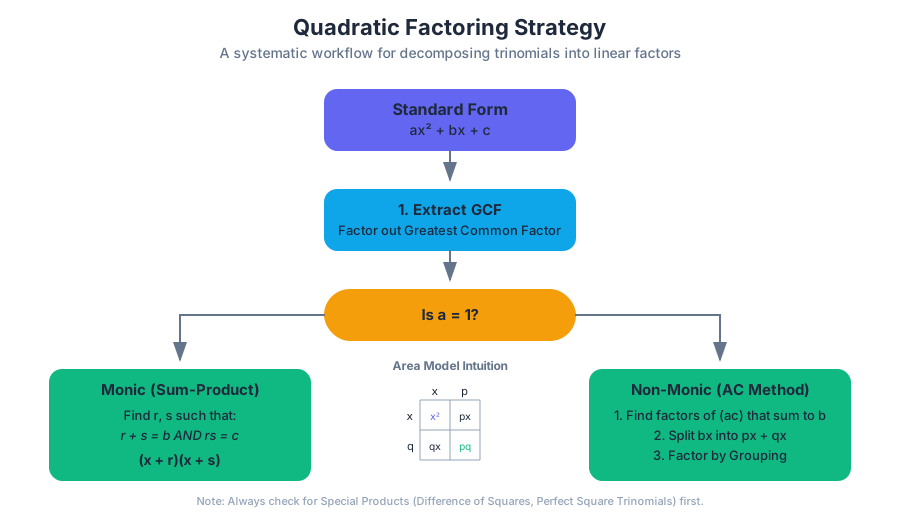
Before diving into abstract coefficients, we must ground the multiplication of binomials in geometry. The Area Model (or box method) treats the product of two binomials, such as $(x + p)(x + q)$, as the area of a rectangle with side lengths $(x + p)$ and $(x + q)$.

How it Works

1. Draw a 2x2 grid.
2. Place the terms of the first binomial along the top.
3. Place the terms of the second binomial along the side.
4. Calculate the area of each individual cell by multiplying the corresponding row and column headers.
5. Sum the four interior areas to find the total expression.

Theorem (The Distributive Property Extension): For any real numbers $x, a, b, c, d$, the product $(ax + b)(cx + d)$ is given by $acx^2 + (ad + bc)x + bd$.

Comparison of Expansion Methods

Method	Visual Intuition	Scalability	Risk of Error
FOIL (First, Outer, Inner, Last)	Low (Mnemonic-based)	Poor (Binomials only)	High (Easy to miss terms)
Area Model	High (Geometric)	Excellent (Polynomials)	Low (Grid enforces completeness)
Distributive Property	Moderate (Algebraic)	Good	Moderate

Factoring Trinomials with Leading Coefficient $a = 1$

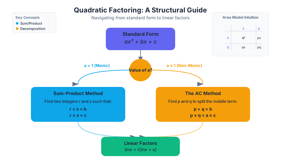
When the leading coefficient $a$ is 1, the expression simplifies to $x^2 + bx + c$. This is known as a monic quadratic. The goal is to find two integers, $r$ and $s$, such that: $$(x + r)(x + s) = x^2 + (r + s)x + rs$$

This implies a system of two equations:

1. $r + s = b$ (The sum of the factors must equal the linear coefficient)
2. $rs = c$ (The product of the factors must equal the constant term)

Worked Example: $x^2 - 5x + 6$

• Identify $b$ and $c$: $b = -5$, $c = 6$.
• List factors of $c$: (1, 6), (-1, -6), (2, 3), (-2, -3).
• Find the pair that sums to $b$: $-2 + (-3) = -5$.
• Result: $(x - 2)(x - 3)$.

Pattern Recognition for Signs

Sign of $c$	Sign of $b$	Factors of $c$	Example
Positive (+)	Positive (+)	Both positive	$x^2 + 5x + 6 = (x+2)(x+3)$
Positive (+)	Negative (-)	Both negative	$x^2 - 5x + 6 = (x-2)(x-3)$
Negative (-)	Positive (+)	One (+) One (-); larger is (+)	$x^2 + x - 6 = (x+3)(x-2)$
Negative (-)	Negative (-)	One (+) One (-); larger is (-)	$x^2 - x - 6 = (x-3)(x+2)$

def factor_monic_trinomial(b, c):
    """
    Finds integers r and s such that r + s = b and r * s = c.
    This is a low-level implementation of the sum-product algorithm.
    """
    factors_of_c = []
    abs_c = abs(c)
    
    # Generate all factor pairs of c
    for i in range(1, int(abs_c**0.5) + 1):
        if abs_c % i == 0:
            factors_of_c.append((i, c // i))
            factors_of_c.append((-i, -c // i))
            
    # Check which pair sums to b
    for r, s in factors_of_c:
        if r + s == b:
            return sorted((r, s))
            
    return None # Irreducible over integers

# Example: x^2 - 5x + 6 -> b=-5, c=6
print(f"Factors: {factor_monic_trinomial(-5, 6)}") 
# Output: [-3, -2]

Factoring by Grouping

Factoring by grouping is a prerequisite for the AC Method (used when $a \neq 1$). It is used when an expression has four terms and no common factor exists for all four, but pairs of terms share commonalities.

The Algorithm

1. Group the first two terms and the last two terms.
2. Factor out the Greatest Common Factor (GCF) from each group.
3. If the remaining binomial factors are identical, factor out that binomial.

Example: $3x^3 - 6x^2 + 5x - 10$

1. Group: $(3x^3 - 6x^2) + (5x - 10)$
2. GCF extraction: $3x^2(x - 2) + 5(x - 2)$
3. Final Factorization: $(3x^2 + 5)(x - 2)$

Pitfall Alert: When the third term is negative, you must be careful with signs. For example, in $x^3 + 3x^2 - 4x - 12$, you must factor out a $-4$ from the second group: $x^2(x + 3) - 4(x + 3) = (x^2 - 4)(x + 3)$.

Factoring Trinomials with $a \neq 1$: The AC Method

When the leading coefficient is not 1, we use the AC Method. This technique transforms a trinomial into a four-term polynomial that can be factored by grouping.

The Derivation

Given $ax^2 + bx + c$, we seek to split the middle term $bx$ into $px + qx$ such that the resulting expression $ax^2 + px + qx + c$ is factorable by grouping. For this to work, the product of the split coefficients $pq$ must equal the product of the outer coefficients $ac$.

\begin{aligned}
&\text{Given: } ax^2 + bx + c \\
&\text{Goal: Find } p, q \text{ such that } p+q=b \text{ and } pq=ac \\
&\text{Rewrite: } ax^2 + px + qx + c \\
&\text{Factor by Grouping: } (ax^2 + px) + (qx + c)
\end{aligned}

Worked Example: $2x^2 + 7x + 3$

1. Identify $a, b, c$: $a=2, b=7, c=3$.
2. Calculate $ac$: $2 \times 3 = 6$.
3. Find factors of 6 that sum to 7: 6 and 1.
4. Split the middle term: $2x^2 + 6x + 1x + 3$.
5. Group and factor: $(2x^2 + 6x) + (1x + 3) \Rightarrow 2x(x + 3) + 1(x + 3)$.
6. Final result: $(2x + 1)(x + 3)$.

Special Products and Patterns

Certain quadratic structures appear frequently in mathematics and physics. Recognizing these "shortcuts" is essential for efficiency.

1. Difference of Squares

The pattern $a^2 - b^2$ always factors into $(a - b)(a + b)$. This is derived from the fact that the "outer" and "inner" terms of the expansion cancel each other out.

Note: $a^2 + b^2$ (Sum of Squares) is irreducible over the set of real numbers. It requires complex numbers to factor: $(a + bi)(a - bi)$.

2. Perfect Square Trinomials

These result from squaring a binomial: $(a + b)^2 = a^2 + 2ab + b^2$ or $(a - b)^2 = a^2 - 2ab + b^2$.

Identification Criteria:

• The first and last terms are perfect squares ($a^2$ and $b^2$).
• The middle term is exactly twice the product of the square roots of the first and last terms ($2ab$).

Special Pattern Summary

Pattern Name	Expression	Factored Form
Difference of Squares	$x^2 - 49$	$(x - 7)(x + 7)$
Perfect Square (Sum)	$x^2 + 10x + 25$	$(x + 5)^2$
Perfect Square (Diff)	$x^2 - 12x + 36$	$(x - 6)^2$
Sum of Squares	$x^2 + 16$	Irreducible (over $\mathbb{R}$)

Advanced Factoring: Structural Recognition

Sometimes an expression does not look like a quadratic at first glance but shares the same underlying structure. This is often solved using u-substitution.

Example: $x^4 - 5x^2 + 4$

This is a "quadratic in form." If we let $u = x^2$, the expression becomes: $$u^2 - 5u + 4$$ Factoring the $u$-expression: $$(u - 4)(u - 1)$$ Substituting $x^2$ back in: $$(x^2 - 4)(x^2 - 1)$$ Applying the Difference of Squares to both: $$(x - 2)(x + 2)(x - 1)(x + 1)$$

Computational Implementation and Verification

In professional engineering or data science contexts, manual factoring is replaced by symbolic computation libraries. These libraries use sophisticated algorithms like the Berlekamp Algorithm or the Cantor-Zassenhaus Algorithm to factor polynomials over finite fields or rational numbers.

import sympy as sp

# Define the symbol
x = sp.Symbol('x')

# Define a complex quadratic expression
expr = 12*x**2 + 11*x - 5

# Factor using SymPy's robust polynomial engine
factored_expr = sp.factor(expr)

print(f"Original: {expr}")
print(f"Factored: {factored_expr}")
# Output: (3*x - 1)*(4*x + 5)

# Verification through expansion
print(f"Verified: {sp.expand(factored_expr) == expr}")

For quick verification in a Unix-like environment, one can use the maxima computer algebra system via the command line:

# Using maxima to factor a polynomial from the CLI
echo "factor(6*x^2 + 19*x + 10);" | maxima --very-quiet
# Output: (x+2)*(6*x+5)

Common Pitfalls and Troubleshooting

1. Ignoring the GCF: Always check for a Greatest Common Factor first. Factoring $2x^2 + 10x + 12$ is much easier if you first factor out the 2: $2(x^2 + 5x + 6) = 2(x+2)(x+3)$.
2. Sign Errors in Grouping: When factoring $(ax^2 + bx) - (cx + d)$, remember that the negative sign applies to the entire second group.
3. Prime Polynomials: Not every quadratic can be factored into linear factors with integer coefficients. If the discriminant ($b^2 - 4ac$) is not a perfect square, the factors will involve radicals or complex numbers.
4. Incomplete Factoring: Always check if your resulting factors can be factored further (e.g., a difference of squares hidden inside a result).

Complex Numbers

The evolution of number systems has always been driven by the necessity to solve equations that were previously deemed "impossible." Just as the introduction of negative numbers allowed for the solution of $x + 5 = 2$, and irrational numbers solved $x^2 = 2$, Complex Numbers emerge as the essential expansion required to solve quadratic equations where the discriminant is negative.

In a complex number system, we move beyond the one-dimensional real number line into a two-dimensional plane, providing a framework that is not only mathematically elegant but also fundamental to modern physics, control theory, and digital signal processing.

The Ontological Expansion: Roots of Negative Numbers

For centuries, mathematicians encountered expressions like $\sqrt{-16}$ and dismissed them as "sophist" or "impossible." If you square any real number—whether positive, negative, or zero—the result is never negative. This created a logical ceiling for algebraic completeness.

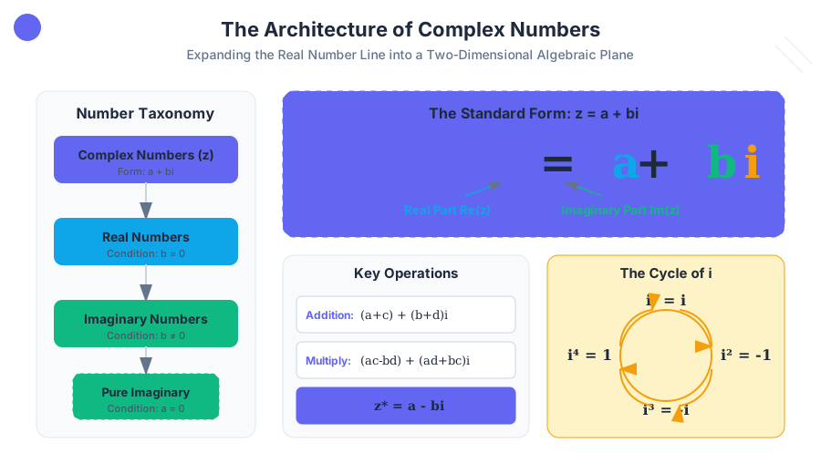
To break this ceiling, we define the imaginary unit, denoted by $i$.

Definition: The Imaginary Unit The imaginary unit $i$ is defined such that: $$i^2 = -1$$ Consequently, $i = \sqrt{-1}$.

Using this definition, we can express the square root of any negative number in terms of $i$. For any positive real number $b$: $$\sqrt{-b} = \sqrt{-1 \cdot b} = \sqrt{-1} \cdot \sqrt{b} = i\sqrt{b}$$

The Cyclic Nature of $i$

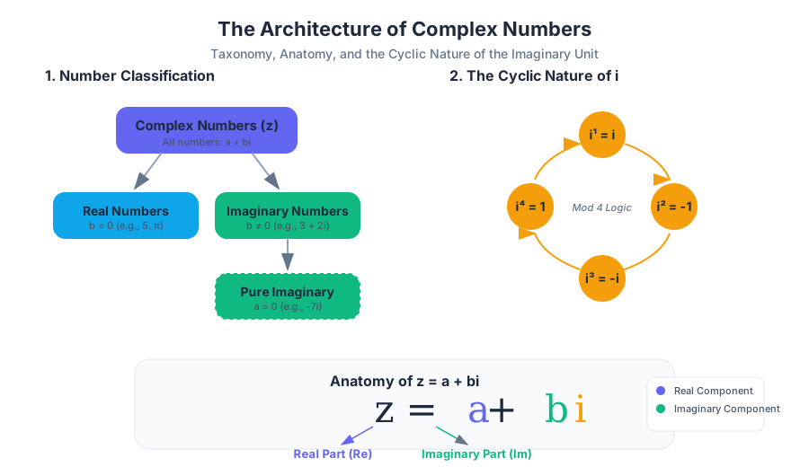
One of the most unique properties of $i$ is its cyclic behavior when raised to integer powers. This periodicity of 4 allows for the rapid simplification of high-degree imaginary expressions.

Power of $i$	Simplification	Result
$i^1$	$\sqrt{-1}$	$i$
$i^2$	$(\sqrt{-1})^2$	$-1$
$i^3$	$i^2 \cdot i = -1 \cdot i$	$-i$
$i^4$	$i^2 \cdot i^2 = (-1)(-1)$	$1$
$i^5$	$i^4 \cdot i$	$i$

Algorithm for $i^n$: To find $i^n$, divide $n$ by 4 and look at the remainder ($r$). The result is $i^r$.

Defining the Complex Number $a + bi$

A Complex Number is any number that can be expressed in the form $z = a + bi$, where $a$ and $b$ are real numbers.

• $a$ is the Real Part, denoted as $\text{Re}(z)$.
• $bi$ is the Imaginary Part, where $b$ is the Imaginary Coefficient, denoted as $\text{Im}(z)$.

Classification of Numbers

Complex numbers act as a superset of all other number types.

Type	Form	Condition	Example
Real Number	$a + 0i$	$b = 0$	$5, \pi, -2.1$
Imaginary Number	$a + bi$	$b \neq 0$	$3 + 2i$
Pure Imaginary	$0 + bi$	$a = 0, b \neq 0$	$-7i, i\sqrt{2}$

Complex Arithmetic: The Algebra of Two Dimensions

Arithmetic with complex numbers follows the standard laws of algebra (distributive, associative, commutative), with the added constraint that $i^2$ must always be replaced with $-1$.

Addition and Subtraction

Addition and subtraction are performed "component-wise." You combine the real parts and the imaginary parts separately. $$(a + bi) \pm (c + di) = (a \pm c) + (b \pm d)i$$

Multiplication

Multiplication follows the FOIL (First, Outer, Inner, Last) method used for binomials. $$(a + bi)(c + di) = ac + adi + bci + bdi^2$$ Since $i^2 = -1$, the last term $bdi^2$ becomes $-bd$. $$(a + bi)(c + di) = (ac - bd) + (ad + bc)i$$

Low-Level Implementation

In systems programming (like C), complex numbers are often represented as structures. Because the hardware doesn't "know" what $i$ is, we must explicitly define the logic for these operations.

#include <stdio.h>

// Define a structure to represent a complex number
typedef struct {
    double real;
    double imag;
} Complex;

// Function to multiply two complex numbers
// Logic: (a+bi)(c+di) = (ac - bd) + (ad + bc)i
Complex multiply_complex(Complex z1, Complex z2) {
    Complex result;
    result.real = (z1.real * z2.real) - (z1.imag * z2.imag);
    result.imag = (z1.real * z2.imag) + (z1.imag * z2.real);
    return result;
}

int main() {
    Complex a = {3.0, 2.0};  // 3 + 2i
    Complex b = {1.0, -4.0}; // 1 - 4i
    
    Complex res = multiply_complex(a, b);
    
    // Expected: (3*1 - 2*-4) + (3*-4 + 2*1)i = (3 + 8) + (-12 + 2)i = 11 - 10i
    printf("Result: %.1f + %.1fi\n", res.real, res.imag);
    return 0;
}

The Complex Conjugate and Division

Division of complex numbers is not as straightforward as real division. To divide by a complex number, we must "realize" the denominator (remove the imaginary component). This is achieved using the Complex Conjugate.

The Conjugate

For any complex number $z = a + bi$, its conjugate, denoted as $\bar{z}$ or $z^*$, is: $$\bar{z} = a - bi$$

The most critical property of the conjugate is that the product of a complex number and its conjugate is always a non-negative real number: $$(a + bi)(a - bi) = a^2 - abi + abi - b^2i^2 = a^2 + b^2$$

Performing Division

To divide $\frac{a + bi}{c + di}$, multiply both the numerator and the denominator by the conjugate of the denominator ($c - di$).

% Mathematical Derivation of Complex Division
\begin{aligned}
\frac{z_1}{z_2} &= \frac{a + bi}{c + di} \\
&= \frac{(a + bi)(c - di)}{(c + di)(c - di)} \\
&= \frac{(ac + bd) + (bc - ad)i}{c^2 + d^2} \\
&= \left(\frac{ac + bd}{c^2 + d^2}\right) + \left(\frac{bc - ad}{c^2 + d^2}\right)i
\end{aligned}

Worked Example: Division

Divide $z_1 = 4 + 2i$ by $z_2 = 3 - i$.

1. Identify the conjugate of the denominator: $\bar{z}_2 = 3 + i$.
2. Multiply numerator and denominator: $$\frac{(4 + 2i)(3 + i)}{(3 - i)(3 + i)}$$
3. Expand the numerator: $$(4 \cdot 3) + (4 \cdot i) + (2i \cdot 3) + (2i \cdot i) = 12 + 4i + 6i - 2 = 10 + 10i$$
4. Expand the denominator: $$3^2 + 1^2 = 9 + 1 = 10$$
5. Simplify: $$\frac{10 + 10i}{10} = 1 + i$$

Geometric Interpretation: The Complex Plane

While real numbers exist on a line, complex numbers exist in the Complex Plane (or Argand Diagram).

• The x-axis represents the Real part.
• The y-axis represents the Imaginary part.

This geometric view transforms complex arithmetic into vector-like operations. Adding $3 + 2i$ to $1 + 4i$ is identical to vector addition in $\mathbb{R}^2$.

Absolute Value (Modulus)

The "size" of a complex number is its distance from the origin $(0,0)$. This is called the modulus, denoted $|z|$. $$|a + bi| = \sqrt{a^2 + b^2}$$

Advanced Applications: Why Complex Numbers Rule the World

In the real world, complex numbers are not "imaginary" in the sense of being fictional. They are the most efficient way to track two related variables simultaneously—specifically magnitude and phase.

Electrical Engineering (AC Circuits)

In Alternating Current (AC) theory, resistance is replaced by Impedance ($Z$). Impedance is a complex number where the real part is resistance ($R$) and the imaginary part is reactance ($X$). $$Z = R + jX$$ (Note: Engineers use $j$ instead of $i$ to avoid confusion with current $I$.)

Signal Processing

The Fourier Transform, which powers everything from JPEG compression to noise-canceling headphones, relies entirely on complex exponentials to decompose signals into frequency components.

import numpy as np

# Real-world usage: Generating a complex signal and finding its magnitude
def analyze_signal(frequency_hz, sampling_rate, duration):
    t = np.linspace(0, duration, int(sampling_rate * duration))
    
    # Create a complex exponential signal: e^(i * 2 * pi * f * t)
    # This represents a rotating phasor in the complex plane
    complex_signal = np.exp(1j * 2 * np.pi * frequency_hz * t)
    
    # In practice, we might add noise
    noise = (np.random.randn(len(t)) + 1j * np.random.randn(len(t))) * 0.1
    dirty_signal = complex_signal + noise
    
    # Calculate the average magnitude (modulus)
    magnitudes = np.abs(dirty_signal)
    avg_mag = np.mean(magnitudes)
    
    print(f"Signal analyzed. Average Modulus: {avg_mag:.4f}")
    return dirty_signal

# Analyze a 60Hz signal (common power line frequency)
signal = analyze_signal(60, 1000, 0.1)

Summary of Operations

Operation	Formula / Method	Result Type
Addition	$(a+c) + (b+d)i$	Complex
Multiplication	$(ac-bd) + (ad+bc)i$	Complex
Conjugation	$\text{flip sign of } bi$	Complex
Modulus	$\sqrt{a^2 + b^2}$	Real
Division	Multiply by $\frac{\bar{z}}{\bar{z}}$	Complex

Common Pitfalls and Edge Cases

1. The Square Root Product Fallacy: A common mistake is assuming $\sqrt{-a} \cdot \sqrt{-b} = \sqrt{(-a)(-b)} = \sqrt{ab}$.

   • Incorrect: $\sqrt{-4} \cdot \sqrt{-9} = \sqrt{36} = 6$.
   • Correct: $\sqrt{-4} \cdot \sqrt{-9} = (2i) \cdot (3i) = 6i^2 = -6$.
   • Rule: Always convert to $i$ form before performing multiplication or division.

2. Neglecting the $i^2$: Students often forget to flip the sign of the last term in a FOIL expansion. $bdi^2$ is always $-bd$.

3. The "Imaginary" Misnomer: The term "imaginary" was coined by René Descartes as a derogatory term. In modern science, these numbers are as "real" as any other; they simply describe rotations and oscillations more efficiently than standard coordinates.

4. Complex Numbers in Denominators: A final answer is generally not considered "simplified" if there is an $i$ in the denominator. Always use the conjugate to rationalize.

Exponents and Exponential Growth

In the hierarchy of arithmetic operations, exponentiation represents the leap from additive scaling to multiplicative scaling. While multiplication is defined as repeated addition, exponentiation is defined as repeated multiplication. This shift in logic introduces non-linear dynamics that govern the most powerful forces in the natural and financial worlds—from the fission of atoms and the spread of viral pathogens to the accumulation of generational wealth through compound interest.

This article provides a rigorous exploration of the algebraic properties of exponents, the mechanics of radical simplification, and the functional behavior of exponential growth and decay models.

The Algebra of Exponents: Fundamental Laws

At its most basic, an exponential expression consists of a base ($b$) raised to a power or exponent ($n$), written as $b^n$. This notation signifies that the base is multiplied by itself $n$ times. However, as we move into college-level algebra, we must extend this definition beyond positive integers to include zero, negative integers, and rational numbers.

The Axioms of Exponentiation

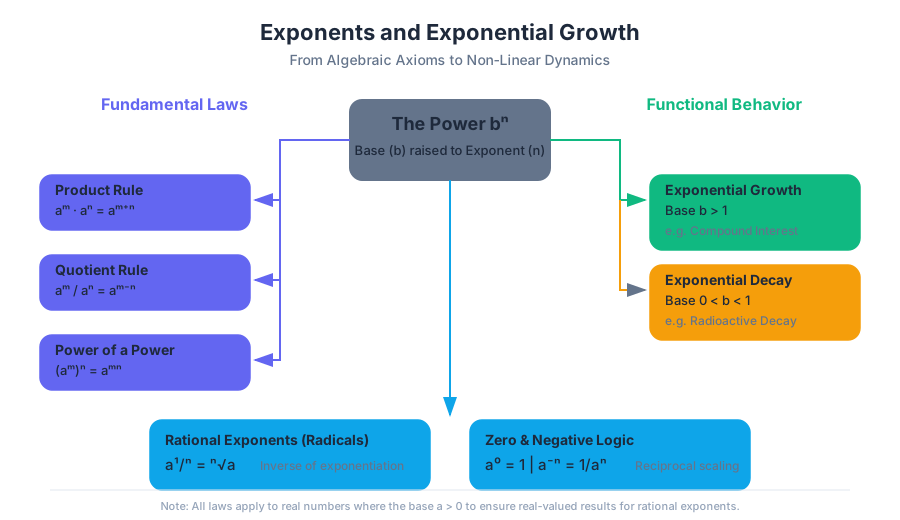
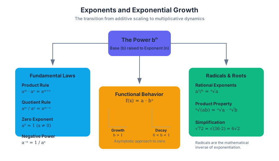
The behavior of exponents is governed by a set of consistent algebraic laws. These are not merely arbitrary rules but are derived from the definition of multiplication.

Law Name	Mathematical Notation	Description
Product Rule	$a^m \cdot a^n = a^{m+n}$	To multiply powers with the same base, add the exponents.
Quotient Rule	$\frac{a^m}{a^n} = a^{m-n}$	To divide powers with the same base, subtract the exponents.
Power of a Power	$(a^m)^n = a^{m \cdot n}$	To raise a power to another power, multiply the exponents.
Power of a Product	$(ab)^n = a^n b^n$	The power of a product is the product of the powers.
Zero Exponent	$a^0 = 1, (a \neq 0)$	Any non-zero base raised to the power of zero is exactly one.
Negative Exponent	$a^{-n} = \frac{1}{a^n}$	A negative exponent represents the reciprocal of the base raised to the positive power.

Derivation: Why is $a^0 = 1$?

Students often find the zero-exponent rule counterintuitive. However, it is a logical necessity of the Quotient Rule. Consider the expression $\frac{x^3}{x^3}$.

1. By basic arithmetic, any non-zero number divided by itself is $1$.
2. By the Quotient Rule, $\frac{x^3}{x^3} = x^{3-3} = x^0$.
3. Therefore, to maintain mathematical consistency, $x^0$ must equal $1$.

Implementation: Numerical Simulation of Growth

In computational science, we often need to model these properties over large datasets. The following Python implementation demonstrates how the product rule is utilized in a simulation of cellular mitosis.

import numpy as np

def simulate_mitosis(initial_cells, generations):
    """
    Simulates cell doubling using the property: 
    Total = initial * 2^generations
    """
    # Using numpy for vectorized exponentiation
    generations_array = np.arange(0, generations + 1)
    population = initial_cells * (2 ** generations_array)
    
    return population

# Example: Start with 10 cells, simulate 10 generations
initial_count = 10
gen_count = 10
results = simulate_mitosis(initial_count, gen_count)

for gen, count in enumerate(results):
    print(f"Generation {gen}: {count} cells")

Radicals and Rational Exponents

A radical is the mathematical inverse of an exponent. While $3^2 = 9$, the square root of $9$ ($\sqrt{9}$) returns us to $3$. In advanced algebra, we treat radicals as rational exponents, which allows us to apply all the standard exponent laws to roots.

Definition: The Principal $n$-th Root For any real number $a$ and positive integer $n$, $a^{1/n} = \sqrt[n]{a}$. If $n$ is even, $a$ must be non-negative for the result to be a real number.

Simplification of Radicals

Simplifying a radical involves removing any perfect $n$-th powers from the radicand (the expression under the radical symbol). This is achieved through the Product Property of Radicals: $\sqrt[n]{ab} = \sqrt[n]{a} \cdot \sqrt[n]{b}$.

Table: Radical Simplification Logic

Expression	Goal	Method	Simplified Result
$\sqrt{72}$	Find largest perfect square	$\sqrt{36 \cdot 2} = \sqrt{36} \cdot \sqrt{2}$	$6\sqrt{2}$
$\sqrt[3]{54}$	Find largest perfect cube	$\sqrt[3]{27 \cdot 2} = \sqrt[3]{27} \cdot \sqrt[3]{2}$	$3\sqrt[3]{2}$
$\sqrt{x^5}$	Extract even powers	$\sqrt{x^4 \cdot x} = x^{4/2} \sqrt{x}$	$x^2\sqrt{x}$

Mathematical Derivation: Rationalizing the Denominator

In formal mathematics, it is standard practice to ensure the denominator of a fraction does not contain a radical. This is called rationalizing.

% Representation of rationalizing a denominator via a conjugate
\text{Given: } \frac{1}{\sqrt{a} + \sqrt{b}} \\
\text{Multiply by the conjugate: } \frac{1(\sqrt{a} - \sqrt{b})}{(\sqrt{a} + \sqrt{b})(\sqrt{a} - \sqrt{b})} \\
\text{Expand the denominator: } \frac{\sqrt{a} - \sqrt{b}}{(\sqrt{a})^2 - (\sqrt{b})^2} \\
\text{Result: } \frac{\sqrt{a} - \sqrt{b}}{a - b}

Exponential Functions: Growth and Decay

An exponential function is a function of the form $f(x) = a \cdot b^x$, where $a$ is the initial value (the y-intercept), $b$ is the base (the growth factor), and $x$ is the exponent (usually representing time).

Distinguishing Growth from Decay

The behavior of the function is entirely determined by the value of the base $b$.

Base Condition	Type	Behavior	Real-World Example
$b > 1$	Exponential Growth	Increases at an accelerating rate.	Population growth, Compound interest.
$0 < b < 1$	Exponential Decay	Decreases, approaching zero asymptotically.	Radioactive decay, Asset depreciation.
$b = 1$	Constant	A horizontal line at $f(x) = a$.	No change over time.

The Mechanics of the Growth Factor

In many word problems, the base $b$ is not given directly but is expressed as a percentage rate of change ($r$).

• For growth: $b = 1 + r$
• For decay: $b = 1 - r$

The Asymptotic Property Exponential functions of the form $f(x) = ab^x$ possess a horizontal asymptote at $y=0$. This means that while the value of the function may become infinitesimally small (in decay) or start extremely flat (in growth), it will never actually touch or cross the x-axis unless a vertical shift is applied.

Modeling with the Natural Base $e$

In the study of continuous processes, we encounter the irrational number $e$ (Euler's number), approximately equal to $2.71828$. This constant arises when we consider the limit of compound interest as the number of compounding periods approaches infinity.

Continuous Compound Interest Formula

The formula for continuous growth is: $$A = Pe^{rt}$$ Where:

• $P$ = Principal (initial amount)
• $e$ = Euler's number
• $r$ = Annual interest rate (decimal)
• $t$ = Time in years

Real-World Usage: Financial Analysis

Engineers and financial analysts often use command-line tools or specialized libraries to calculate these values with high precision.

# Using the 'bc' arbitrary precision calculator in a shell script
# To calculate the value of $1000 at 5% interest compounded continuously for 10 years
# Formula: 1000 * e^(0.05 * 10)

echo "scale=5; 1000 * e(0.05 * 10)" | bc -l

# Output: 1648.72127

Advanced Topic: Binary Exponentiation

In computer science, calculating $a^b$ where $b$ is a very large integer (as seen in RSA encryption) using the naive method of $b$ multiplications is inefficient ($O(n)$). Instead, we use Binary Exponentiation (also known as Square and Multiply), which reduces the complexity to $O(\log n)$.

Implementation: Fast Power Algorithm

#include <stdio.h>

/**
 * Calculates (base^exp) % mod efficiently.
 * This is the backbone of modern cryptography.
 */
long long power(long long base, long long exp, long long mod) {
    long long res = 1;
    base = base % mod;
    while (exp > 0) {
        // If exp is odd, multiply base with result
        if (exp % 2 == 1) res = (res * base) % mod;
        
        // exp must be even now
        base = (base * base) % mod;
        exp = exp / 2;
    }
    return res;
}

int main() {
    printf("Result: %lld\n", power(2, 10, 1000000)); // 2^10 = 1024
    return 0;
}

Common Pitfalls and Misconceptions

1. The "Freshman's Dream": A very common error is assuming $(a + b)^n = a^n + b^n$. This is false for all $n > 1$. For example, $(2+3)^2 = 5^2 = 25$, but $2^2 + 3^2 = 4 + 9 = 13$.
2. Negative Base vs. Negative Exponent: A negative exponent ($x^{-2}$) does not make the result negative; it creates a reciprocal ($1/x^2$). A negative base ($(-x)^2$) may or may not be negative depending on whether the exponent is even or odd.
3. Order of Operations: In the expression $-3^2$, the exponent applies only to the $3$, resulting in $-9$. To square the negative number, parentheses are required: $(-3)^2 = 9$.
4. Linear vs. Exponential Growth: In a linear model, the amount of change is constant. In an exponential model, the percentage of change is constant.

Summary of Applications

The mastery of exponents and radicals is not merely an academic exercise; it is the prerequisite for understanding Logarithms, which are the inverse of exponential functions. Without these tools, we could not measure the magnitude of earthquakes (Richter scale), the acidity of liquids (pH scale), or the brightness of stars (apparent magnitude).

Field	Application	Model Type
Biology	Bacterial culture growth	Exponential Growth
Chemistry	Half-life of Carbon-14	Exponential Decay
Finance	Inflation and Purchasing Power	Exponential Decay
Data Science	Complexity of algorithms	Power Laws
Physics	Newton's Law of Cooling	Exponential Decay

Rational Expressions and Equations

In the hierarchy of algebraic structures, rational expressions represent the formal extension of polynomials into the realm of division, analogous to how rational numbers extend the integers. A rational expression is defined as the quotient of two polynomials, $P(x)$ and $Q(x)$, expressed in the form $\frac{P(x)}{Q(x)}$, where $Q(x) \neq 0$.

Mastering this domain is not merely an exercise in symbolic manipulation; it is a prerequisite for calculus, where rational functions describe asymptotic behavior, and for engineering, where they model everything from fluid dynamics to electrical impedance. This article provides a rigorous deep-dive into the mechanics of reducing these expressions, performing complex arithmetic, and solving the transcendental equations that arise in real-world rate and mixture modeling.

Foundations of Rational Expressions

A rational expression is inherently tied to its domain. Unlike polynomials, which are defined for all real numbers, a rational expression is undefined wherever the denominator polynomial $Q(x)$ evaluates to zero. These values are known as excluded values or singularities.

The Fundamental Principle of Fractions: For any polynomials $P, Q,$ and $R$ (where $Q, R \neq 0$), the equality $\frac{P \cdot R}{Q \cdot R} = \frac{P}{Q}$ holds for all values in the domain. This principle is the mathematical basis for both simplification (reduction) and finding common denominators.

Domain Restrictions and Continuity

Before any algebraic reduction occurs, one must identify the domain. If an expression $\frac{x-2}{(x-2)(x+3)}$ is simplified to $\frac{1}{x+3}$, the value $x=2$ remains excluded from the original function's domain, creating a "removable discontinuity" or a "hole" in the graph.

Feature	Polynomial Expression	Rational Expression
Domain	All real numbers $(-\infty, \infty)$	Restricted where $Q(x) = 0$
End Behavior	Approaches $\pm\infty$	Often approaches a horizontal asymptote
Complexity	Linear/Quadratic/Higher Degree	Ratio of degrees (Relative complexity)
Arithmetic	Closed under $+$, $-$, $\times$	Closed under $+$, $-$, $\times$, and $\div$

Reducing Rational Expressions

Reducing a rational expression to its lowest terms requires the complete factorization of both the numerator and the denominator. The process relies on identifying common factors that constitute a "form of one" (e.g., $\frac{x+5}{x+5} = 1$).

The Reduction Algorithm

1. Factor Completely: Decompose both $P(x)$ and $Q(x)$ into irreducible factors over the real numbers.
2. Identify the Domain: Note all values that make the original denominator zero.
3. Cancel Common Factors: Divide out factors present in both the numerator and denominator.
4. State the Simplified Result: Provide the reduced expression along with the original domain restrictions.

# Low-level implementation: Symbolic Simplification Logic
# This script demonstrates how a computer algebra system (CAS) 
# might represent and reduce a rational expression.

class Polynomial:
    def __init__(self, factors):
        # Represented as a list of roots/factors for simplicity
        # e.g., (x-2)(x+3) -> [2, -3]
        self.factors = sorted(factors)

    def simplify_with(self, other):
        """Reduces the fraction self / other."""
        common_factors = []
        new_num = list(self.factors)
        new_den = list(other.factors)
        
        # Intersection logic to find common factors
        for factor in self.factors:
            if factor in new_den:
                common_factors.append(factor)
                new_num.remove(factor)
                new_den.remove(factor)
        
        return new_num, new_den, common_factors

# Example: (x-2)(x+5) / (x-2)(x+1)
numerator = Polynomial([2, -5])
denominator = Polynomial([2, -1])
num, den, excluded = numerator.simplify_with(denominator)

print(f"Simplified Numerator Roots: {num}")
print(f"Simplified Denominator Roots: {den}")
print(f"Excluded Values (Holes): {excluded}")

Rational Arithmetic: Multiplication and Division

The operations of multiplication and division for rational expressions follow the same logic as numerical fractions, but with a significantly higher overhead for bookkeeping.

Multiplication

To multiply $\frac{A}{B} \cdot \frac{C}{D}$, we compute $\frac{AC}{BD}$. However, it is computationally and algebraically inefficient to expand these polynomials first. Instead, factor everything first, then simplify across the numerators and denominators.

Division

Division is defined as multiplication by the reciprocal: $$\frac{A}{B} \div \frac{C}{D} = \frac{A}{B} \cdot \frac{D}{C} = \frac{AD}{BC}$$ Crucial Pitfall: When dividing, the domain is restricted by the zeros of $B$, $D$, and $C$ (since $C$ moves to the denominator).

Rational Arithmetic: Addition and Subtraction

Addition and subtraction are the most error-prone operations due to the requirement of a Least Common Denominator (LCD). The LCD of two or more rational expressions is the Least Common Multiple (LCM) of their denominators.

Finding the LCM of Polynomials

To find the LCM, factor each denominator completely. The LCM is the product of each unique factor raised to the highest power that appears in any single factorization.

Example:

• Denominator 1: $(x+1)^2(x-2)$
• Denominator 2: $(x+1)(x-2)(x+5)$
• LCM: $(x+1)^2(x-2)(x+5)$

The "Building Factor" Method

Once the LCD is identified, each fraction must be multiplied by a "building factor"—a fraction equal to 1 composed of the factors missing from its current denominator to match the LCD.

Step	Action	Mathematical Representation
1	Factor Denominators	$D_1, D_2, \dots$
2	Determine LCD	$L = \text{lcm}(D_1, D_2)$
3	Multiply by $\frac{L/D_i}{L/D_i}$	$\frac{N_1}{D_1} \cdot \frac{k_1}{k_1} + \frac{N_2}{D_2} \cdot \frac{k_2}{k_2}$
4	Combine Numerators	$\frac{N_1k_1 + N_2k_2}{L}$
5	Simplify	Factor the result and reduce if possible

Solving Rational Equations

A rational equation contains at least one rational expression. The primary strategy for solving these is to "clear the denominators" by multiplying the entire equation by the LCD of all terms.

The Workflow for Solving

1. Identify the LCD of all rational expressions in the equation.
2. Multiply every term by this LCD. This transforms the rational equation into a polynomial equation (linear or quadratic).
3. Solve the resulting polynomial equation.
4. Check for Extraneous Solutions: This is the most critical step. Any solution that makes a denominator in the original equation zero must be discarded.

\text{Solve: } \frac{3}{x-2} + \frac{1}{x} = \frac{2}{x-2}

\text{1. LCD is } x(x-2). \text{ Excluded: } x \neq 0, 2.
\text{2. Multiply by } x(x-2):
   x(x-2) \left[ \frac{3}{x-2} \right] + x(x-2) \left[ \frac{1}{x} \right] = x(x-2) \left[ \frac{2}{x-2} \right]
\text{3. Simplify:}
   3x + (x-2) = 2x
\text{4. Solve:}
   4x - 2 = 2x \implies 2x = 2 \implies x = 1
\text{5. Verify:}
   x=1 \text{ is not in the excluded set } \{0, 2\}. \text{ Solution is valid.}

Modeling with Combined Rates (Work Problems)

Rational equations are the standard tool for solving "work" problems, where multiple entities complete a task at different constant rates.

The Work Formula

If an entity completes a task in $t$ hours, its rate is $\frac{1}{t}$ tasks per hour. When multiple entities work together, their rates are additive: $$\frac{1}{t_1} + \frac{1}{t_2} + \dots + \frac{1}{t_n} = \frac{1}{t_{total}}$$ This is essentially the Harmonic Mean formula.

Key Insight: We do not add the times; we add the rates. If Pipe A fills a tank in 3 hours and Pipe B in 6 hours, the combined time is not 9 hours, but rather the solution to $\frac{1}{3} + \frac{1}{6} = \frac{1}{t}$, which yields $t=2$.

Modeling Mixture Problems

Mixture problems involve combining two or more substances with different concentrations to reach a target concentration. These are modeled using the principle of Conservation of Mass.

The Concentration Equation

The amount of "pure" substance in a mixture is the product of the concentration ($C$) and the total volume ($V$). $$C_1V_1 + C_2V_2 = C_fV_f$$ Where $V_f = V_1 + V_2$. When solving for an unknown volume to be added, the equation often becomes rational: $$C_f = \frac{C_1V_1 + C_2V_2}{V_1 + V_2}$$

Mixture Problem Parameters

Variable	Definition	Typical Units
$C$	Concentration	%, Molarity, or Ratio
$V$	Volume/Amount	Liters, Grams, Gallons
$C \cdot V$	Pure Substance	Mass or Volume of solute
$V_{added}$	Variable to solve	The "x" in most equations

/**
 * Real-world usage: A Concentration Calculator Logic
 * Used in a laboratory UI to determine how much stock solution to add.
 */
interface MixtureResult {
  requiredVolume: number;
  finalVolume: number;
}

function calculateRequiredVolume(
  currentVolume: number,
  currentConcentration: number, // e.g., 0.10 for 10%
  targetConcentration: number,
  stockConcentration: number
): MixtureResult {
  // Equation: (C1*V1 + Cs*Vs) / (V1 + Vs) = Ct
  // Solving for Vs:
  // C1*V1 + Cs*Vs = Ct*V1 + Ct*Vs
  // Vs(Cs - Ct) = V1(Ct - C1)
  // Vs = V1(Ct - C1) / (Cs - Ct)

  if (stockConcentration <= targetConcentration) {
    throw new Error("Stock concentration must be higher than target.");
  }

  const vs = (currentVolume * (targetConcentration - currentConcentration)) / 
             (stockConcentration - targetConcentration);

  return {
    requiredVolume: Math.round(vs * 100) / 100,
    finalVolume: Math.round((currentVolume + vs) * 100) / 100
  };
}

// Example: We have 500ml of 10% saline. We need it to be 15%. 
// We are adding 30% stock saline.
const result = calculateRequiredVolume(500, 0.10, 0.15, 0.30);
console.log(`Add ${result.requiredVolume}ml of stock.`);

Common Pitfalls and Advanced Considerations

1. The Sign Error in Subtraction

When subtracting a rational expression with a polynomial numerator, such as $-\frac{x-5}{x+2}$, the negative sign must be distributed to every term in the numerator: $\frac{-(x-5)}{x+2} = \frac{-x+5}{x+2}$. Failure to distribute is the single most common error in rational arithmetic.

2. Extraneous Solutions

In the process of clearing denominators, we multiply by a variable expression. If that expression equals zero at the calculated solution, we have effectively multiplied both sides of the equation by zero, which is an invalid algebraic move. Always cross-reference solutions with the initial domain restrictions.

3. Complex Fractions

A "complex fraction" is a rational expression where the numerator or denominator (or both) also contain rational expressions. These are best handled by multiplying the "big" numerator and "big" denominator by the LCD of all "small" internal fractions.

• Rational Expression: A ratio of two polynomials $P(x)/Q(x)$.
• Excluded Value: A value of $x$ that makes the denominator zero.
• LCD (Least Common Denominator): The smallest polynomial that is a multiple of all denominators in a set.
• Extraneous Solution: A solution derived algebraically that does not satisfy the original equation due to domain restrictions.
• Combined Rate: The sum of individual rates ($\frac{1}{t_1} + \frac{1}{t_2}$) used to find total time.
• Removable Discontinuity: A "hole" in a graph occurring at a value that was canceled out during simplification.

1. Why must we factor the denominators before finding the LCD?
2. If a rational equation simplifies to $x=3$, but the original denominator was $(x-3)(x+2)$, what is the solution set?
3. In a work problem, if Person A takes $a$ hours and Person B takes $b$ hours, why is the answer not $(a+b)/2$?
4. How does the domain of $\frac{x^2-9}{x-3}$ differ from the domain of $x+3$?
5. What is the effect of multiplying an equation by the LCD if the LCD is zero for a specific $x$?

Rational Expressions Mastery Checklist

• Can you factor all quadratic patterns (Difference of Squares, Trinomials, GCF)?
• Do you always state the domain before simplifying?
• Can you distinguish between a rational expression (to be simplified) and a rational equation (to be solved)?
• When adding fractions, do you remember to multiply the numerator by the "missing" factors of the LCD?
• In mixture problems, are you consistently using the formula $C_1V_1 + C_2V_2 = C_fV_f$?
• Have you practiced checking for extraneous solutions in every equation?

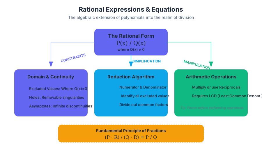
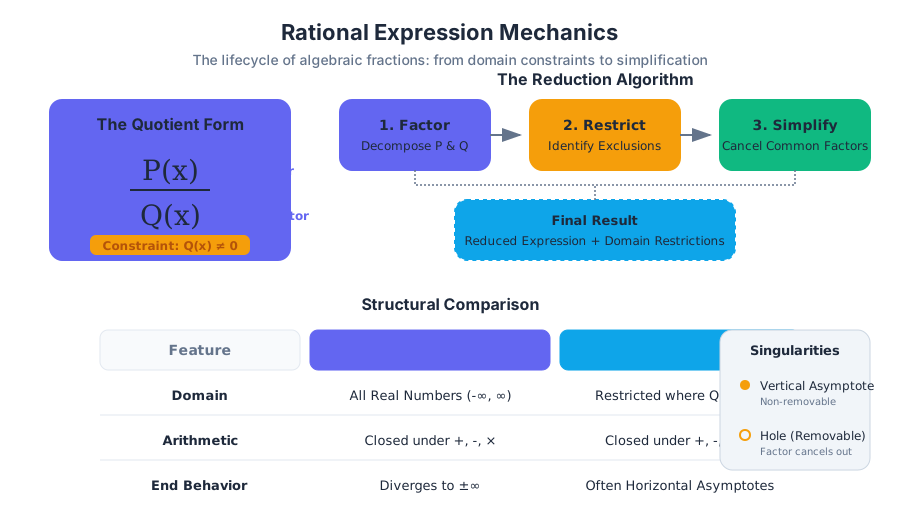
Coordinate Geometry and Circles: The Analytic Bridge

Coordinate geometry, also known as Analytic Geometry, represents one of the most significant leaps in mathematical history. By imposing a Cartesian coordinate system onto Euclidean space, we transform geometric shapes into algebraic equations. This synthesis allows us to solve complex spatial problems using the precision of algebra and, conversely, to visualize algebraic relationships through geometry.

At the heart of this discipline lies the study of the Circle—the locus of all points in a plane that are equidistant from a fixed point. Understanding the circle requires a mastery of the fundamental metrics of the Cartesian plane: distance and division.

The Distance Formula: Quantifying Space

The Distance Formula is the foundational metric of coordinate geometry. It provides a numerical value for the length of the straight-line segment connecting any two points $(x_1, y_1)$ and $(x_2, y_2)$ in a two-dimensional plane.

1. What it is

The distance $d$ between two points $P_1(x_1, y_1)$ and $P_2(x_2, y_2)$ is defined by the formula:

$$d = \sqrt{(x_2 - x_1)^2 + (y_2 - y_1)^2}$$

2. Why it matters

Without the ability to calculate distance, we cannot define circles, parabolas, or ellipses algebraically. In modern engineering, the distance formula is the backbone of Euclidean Norms in machine learning, collision detection in game development, and signal strength calculations in telecommunications.

3. How it works: The Pythagorean Derivation

The formula is not an arbitrary rule; it is a direct application of the Pythagorean Theorem ($a^2 + b^2 = c^2$).

1. Draw a horizontal line from $P_1$ and a vertical line from $P_2$ to form a right-angled triangle.
2. The horizontal leg (base) has a length of $|x_2 - x_1|$.
3. The vertical leg (height) has a length of $|y_2 - y_1|$.
4. The distance $d$ is the hypotenuse. Squaring the legs and taking the square root yields the formula.

4. Implementation in Python

In a computational context, we must handle floating-point precision and potential overflows when dealing with large coordinates.

import math

def calculate_euclidean_distance(p1, p2):
    """
    Calculates the straight-line distance between two points in 2D space.
    p1, p2: Tuples or lists of (x, y)
    """
    try:
        # Using math.dist (available in Python 3.8+) for optimized performance
        # and better numerical stability than manual sqrt((x2-x1)**2 + (y2-y1)**2)
        return math.dist(p1, p2)
    except AttributeError:
        # Fallback for older Python versions
        dx = p2[0] - p1[0]
        dy = p2[1] - p1[1]
        return math.sqrt(dx**2 + dy**2)

# Example usage:
point_a = (3.5, -2.1)
point_b = (10.2, 5.9)
print(f"Distance: {calculate_euclidean_distance(point_a, point_b):.4f}")

5. Common Pitfalls

• Sign Errors: Students often confuse $(x_2 - x_1)$ with $(x_2 + x_1)$. Because the term is squared, the order doesn't matter, but the operation must be subtraction.
• Dimensionality: Forgetting that the formula expands to $\sqrt{\Delta x^2 + \Delta y^2 + \Delta z^2}$ in 3D space.
• Computational Cost: Square root operations are "expensive" for CPUs. In many applications (like comparing distances), developers use the Squared Distance ($d^2$) to avoid the sqrt call.

Feature	Distance Formula	Manhattan Distance (L1)
Path	Straight line (as the crow flies)	Grid-based (city block)
Formula	$\sqrt{\Delta x^2 + \Delta y^2}$	$
Use Case	Physics, Geometry, Graphics	Pathfinding, Robotics, Taxicab geometry
Invariance	Rotationally invariant	Depends on axis orientation

The Midpoint Formula: Finding Equilibrium

The Midpoint Formula identifies the exact center of a line segment. Unlike the distance formula, which yields a scalar (a single number), the midpoint formula yields a vector (a new coordinate).

1. What it is

The midpoint $M(x_m, y_m)$ of a segment with endpoints $(x_1, y_1)$ and $(x_2, y_2)$ is the arithmetic mean of the coordinates:

$$M = \left( \frac{x_1 + x_2}{2}, \frac{y_1 + y_2}{2} \right)$$

2. Why it matters

Midpoints are essential for finding centers of mass, bisecting angles, and determining the center of a circle when only the diameter's endpoints are known. In data science, it is the simplest form of Linear Interpolation (LERP).

3. How it works

Mathematically, the midpoint is the average position. If you are at $x=2$ and your friend is at $x=10$, the middle is $(2+10)/2 = 6$. This logic applies independently to both the $x$ and $y$ axes.

4. Pseudocode Derivation

ALGORITHM FindMidpoint
    INPUT: Point A (x1, y1), Point B (x2, y2)
    
    // Calculate the average of the x-coordinates
    SET midX = (A.x + B.x) / 2
    
    // Calculate the average of the y-coordinates
    SET midY = (A.y + B.y) / 2
    
    OUTPUT: Point(midX, midY)
END ALGORITHM

5. Variations: The Section Formula

The midpoint is a specific case of the Section Formula, which finds a point $P$ that divides a segment in a ratio $m:n$.

$$P = \left( \frac{mx_2 + nx_1}{m+n}, \frac{my_2 + ny_1}{m+n} \right)$$ When $m=1$ and $n=1$, this simplifies to the midpoint formula.

The Standard Equation of a Circle

A circle is defined as the set of all points $(x, y)$ that are a fixed distance $r$ (the radius) from a fixed point $(h, k)$ (the center).

1. What it is

The Standard Form of a circle's equation is:

$$(x - h)^2 + (y - k)^2 = r^2$$

2. Derivation from Distance

If we take the distance formula between a general point $(x, y)$ and the center $(h, k)$, we get: $$\sqrt{(x - h)^2 + (y - k)^2} = r$$ Squaring both sides removes the radical and gives us the standard equation. This is a beautiful example of how a geometric definition (constant distance) becomes an algebraic constraint.

3. Parameters and Their Effects

Parameter	Role	Effect on Graph
$h$	x-coordinate of center	Shifts circle left (if $h < 0$) or right (if $h > 0$)
$k$	y-coordinate of center	Shifts circle down (if $k < 0$) or up (if $k > 0$)
$r$	Radius	Determines the size; must be $> 0$
$r^2$	Squared Radius	The constant on the right side of the equation

4. Real-World Usage: Collision Detection

In game development, checking if two circular objects (like a player and a power-up) are touching is done by comparing the distance between their centers to the sum of their radii.

/**
 * Detects if two circles are overlapping.
 * circleA, circleB: Objects with {x, y, radius}
 */
function isColliding(circleA, circleB) {
    const dx = circleA.x - circleB.x;
    const dy = circleA.y - circleB.y;
    
    // Calculate squared distance to avoid expensive Math.sqrt()
    const distanceSquared = (dx * dx) + (dy * dy);
    const radiusSum = circleA.radius + circleB.radius;
    const radiusSumSquared = radiusSum * radiusSum;

    // If distance between centers is less than the sum of radii, they collide
    return distanceSquared <= radiusSumSquared;
}

const player = { x: 100, y: 150, radius: 20 };
const enemy = { x: 110, y: 160, radius: 15 };

console.log(`Collision: ${isColliding(player, enemy)}`);

The Expanded (General) Equation of a Circle

While the standard form is useful for graphing, circles often appear in an "expanded" or "general" algebraic form where the binomials have been multiplied out.

1. What it is

The General Form of a circle equation is:

$$x^2 + y^2 + Dx + Ey + F = 0$$ Where $D, E,$ and $F$ are constants.

2. Conversion: Completing the Square

To find the center $(h, k)$ and radius $r$ from the general form, we must perform the process of Completing the Square. This is the bridge back to the standard form.

The Process:

1. Group the $x$ terms and $y$ terms together.
2. Move the constant $F$ to the other side of the equation.
3. For both $x$ and $y$, take the coefficient of the linear term ($D$ and $E$), divide by 2, and square it.
4. Add these values to both sides of the equation to maintain equality.
5. Factor the resulting trinomials into perfect squares.

3. Worked Example

Problem: Find the center and radius of $x^2 + y^2 - 6x + 8y + 9 = 0$.

1. Group terms: $(x^2 - 6x) + (y^2 + 8y) = -9$
2. Complete the square for x: $(-6 / 2)^2 = 9$. Add 9 to both sides.
3. Complete the square for y: $(8 / 2)^2 = 16$. Add 16 to both sides.
4. New Equation: $(x^2 - 6x + 9) + (y^2 + 8y + 16) = -9 + 9 + 16$
5. Factor: $(x - 3)^2 + (y + 4)^2 = 16$

Result: Center is $(3, -4)$, Radius is $\sqrt{16} = 4$.

4. Special Cases in General Form

The value of the constant on the right side after completing the square (let's call it $R_{val}$) determines the nature of the graph:

• $R_{val} > 0$: A real circle exists.
• $R_{val} = 0$: The "circle" is actually just a single point (the center).
• $R_{val} < 0$: The equation represents an "imaginary circle" (no real points satisfy the equation).

Equation Type	Form	Best For
Standard Form	$(x-h)^2 + (y-k)^2 = r^2$	Identifying center/radius, graphing
General Form	$x^2 + y^2 + Dx + Ey + F = 0$	Calculus (differentiation), system of equations
Parametric Form	$x = h + r\cos(t), y = k + r\sin(t)$	Computer animation, physics simulations

Advanced Extensions: Tangents and Intersections

Coordinate geometry allows us to solve for the interaction between circles and other geometric entities.

1. Tangent Lines

A line is tangent to a circle if it touches it at exactly one point. A key property is that the radius to the point of tangency is always perpendicular to the tangent line.

• Algebraic Check: Substitute the line equation ($y = mx + b$) into the circle equation. If the resulting quadratic has exactly one solution (discriminant $B^2 - 4AC = 0$), the line is tangent.

2. Intersection of Two Circles

Two circles can intersect at zero, one (tangent circles), or two points. Finding these points involves subtracting one circle equation from another to find the Radical Axis (a linear equation passing through the intersection points), then substituting that line back into one of the circles.

Summary of Formulas

Distance: $d = \sqrt{(x_2-x_1)^2 + (y_2-y_1)^2}$

Midpoint: $M = \left(\frac{x_1+x_2}{2}, \frac{y_1+y_2}{2}\right)$

Standard Circle: $(x-h)^2 + (y-k)^2 = r^2$

General Circle: $x^2 + y^2 + Dx + Ey + F = 0$

• Term: Cartesian Plane Definition: A 2D coordinate system defined by an x-axis and a y-axis.
• Term: Locus Definition: A set of points whose location satisfies or is determined by one or more specified conditions.
• Term: Completing the Square Definition: A technique used to turn a quadratic expression into a perfect square trinomial.
• Term: Radius Definition: The constant distance from the center of a circle to any point on its edge.
• Term: Diameter Endpoints Definition: Two points on a circle such that the segment connecting them passes through the center.
• Term: Radical Axis Definition: The line of points with equal power with respect to two circles; the line where two circles intersect.

1. Conceptual: If you double the radius of a circle in the equation $(x-h)^2 + (y-k)^2 = r^2$, what happens to the constant on the right side of the equation?
2. Calculation: Find the midpoint of the segment with endpoints $(-5, 12)$ and $(7, -4)$.
3. Derivation: Why is the distance formula always positive (or zero), regardless of whether the coordinates are negative?
4. Application: A circle has a diameter with endpoints $(2, 3)$ and $(8, 11)$. What is the standard equation of this circle? (Hint: Use Midpoint for center and Distance for radius).
5. Analysis: Convert $x^2 + y^2 - 10x + 2y + 26 = 0$ into standard form. What kind of geometric object does this represent?

Study Guide: Mastery Checklist

• Derive the Distance Formula: Can you draw the right triangle on a coordinate plane and use $a^2 + b^2 = c^2$ to explain the formula?
• Calculate Midpoints: Can you find the center of a line segment using averages?
• Identify Circle Centers: Given $(x+5)^2 + (y-2)^2 = 49$, can you correctly identify the center as $(-5, 2)$ and NOT $(5, -2)$?
• Complete the Square: Can you transform $x^2 + y^2 + 4x - 6y - 3 = 0$ into standard form without looking at notes?
• Graphing: Can you plot a circle given its equation by first marking the center and then moving $r$ units in the four cardinal directions?
• Real-world Logic: Do you understand why $d^2$ is used in programming instead of $d$ for performance optimization?

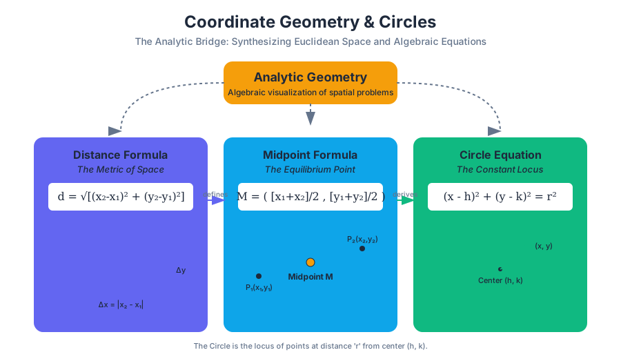
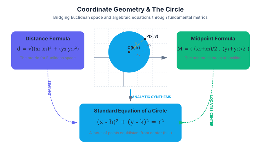
Polynomial Arithmetic

Polynomials serve as the fundamental building blocks of modern analysis, acting as the bridge between elementary arithmetic and the complex landscapes of calculus and abstract algebra. In the rigorous study of mathematics, a polynomial in one variable (typically $x$) is defined as an expression consisting of variables and coefficients, involving only the operations of addition, subtraction, multiplication, and non-negative integer exponents.

Formally, we represent a polynomial $P(x)$ of degree $n$ as: $$P(x) = a_n x^n + a_{n-1} x^{n-1} + \dots + a_1 x + a_0$$ where $a_n, a_{n-1}, \dots, a_0$ are constants (coefficients) and $a_n \neq 0$.

The study of polynomial arithmetic is not merely a set of rules for manipulation; it is the study of the Ring of Polynomials, denoted as $R[x]$. Like integers, polynomials can be added, subtracted, and multiplied to produce another polynomial, demonstrating the property of closure. This section explores the mechanics of these operations, the structural patterns that allow for advanced factoring, and the analytical methods used to describe their behavior over intervals.

Polynomial Addition and Subtraction

At its core, polynomial addition and subtraction are exercises in linear combination. Because polynomials are defined by the powers of their variables, we treat each power $x^k$ as a distinct dimension or "basis vector." We can only combine terms that share the same exponent—these are known as like terms.

The Mechanics of Alignment

To add or subtract polynomials, one must align terms of the same degree. While horizontal alignment is common in casual algebra, vertical alignment is the preferred method for complex, high-degree expressions to prevent "bookkeeping" errors.

The Principle of Superposition: The sum of two polynomials $f(x)$ and $g(x)$ is a new polynomial $h(x)$ where each coefficient $h_i$ is the sum of the corresponding coefficients $f_i$ and $g_i$. Formally: $$(f + g)(x) = \sum_{i=0}^{n} (a_i + b_i)x^i$$

Complexity and Properties

Operation	Complexity (Big O)	Identity Element	Inverse Element
Addition	$O(n)$	$0$	$-P(x)$
Subtraction	$O(n)$	$0$	$P(x)$
Multiplication	$O(n^2)$ or $O(n \log n)$	$1$	N/A (for polynomials)

# Low-level implementation of Polynomial Addition in Python
# Representing polynomials as lists where index i is the coefficient of x^i

def add_polynomials(poly1, poly2):
    """
    Adds two polynomials represented as lists of coefficients.
    Example: [1, 2, 3] represents 1 + 2x + 3x^2
    """
    size = max(len(poly1), len(poly2))
    result = [0] * size
    
    for i in range(size):
        term1 = poly1[i] if i < len(poly1) else 0
        term2 = poly2[i] if i < len(poly2) else 0
        result[i] = term1 + term2
        
    # Remove trailing zeros to maintain canonical form
    while len(result) > 1 and result[-1] == 0:
        result.pop()
        
    return result

# Example: (3x^2 + 2x + 1) + (5x + 4)
p1 = [1, 2, 3]
p2 = [4, 5]
print(f"Resulting Coefficients: {add_polynomials(p1, p2)}") # Expected: [5, 7, 3]

Advanced Factoring Techniques

Factoring is the process of decomposing a polynomial into a product of simpler polynomials. While basic algebra focuses on quadratic trinomials with a leading coefficient of 1, advanced factoring tackles higher-degree expressions and non-trivial structures.

Factoring by Grouping

When a polynomial has four or more terms, grouping is often the first line of defense. This technique involves partitioning the polynomial into two or more sections, extracting the Greatest Common Factor (GCF) from each, and hoping for a common binomial factor.

Example: Factor $x^3 - 3x^2 + 4x - 12$

1. Group: $(x^3 - 3x^2) + (4x - 12)$
2. Factor GCF from each: $x^2(x - 3) + 4(x - 3)$
3. Factor out the common binomial: $(x^2 + 4)(x - 3)$

Special Cubic Patterns

Unlike quadratics, which follow the general trinomial rule, cubic polynomials often follow specific "identities" that must be memorized or derived.

Pattern Name	Formula
Sum of Cubes	$a^3 + b^3 = (a + b)(a^2 - ab + b^2)$
Difference of Cubes	$a^3 - b^3 = (a - b)(a^2 + ab + b^2)$
Perfect Cube (Sum)	$a^3 + 3a^2b + 3ab^2 + b^3 = (a + b)^3$

\begin{aligned}
\text{Derivation of Sum of Cubes:} \\
(a+b)(a^2 - ab + b^2) &= a(a^2 - ab + b^2) + b(a^2 - ab + b^2) \\
&= a^3 - a^2b + ab^2 + ba^2 - ab^2 + b^3 \\
&= a^3 + (-a^2b + a^2b) + (ab^2 - ab^2) + b^3 \\
&= a^3 + b^3
\end{aligned}

Factoring Using Structure

One of the most powerful tools in a mathematician's arsenal is the ability to recognize structure—seeing a complex expression as a variation of a simpler one. This is often achieved through substitution (or $u$-substitution).

Quadratic Form

Many higher-degree polynomials are "quadratic in form." If a polynomial follows the pattern $a[f(x)]^2 + b[f(x)] + c$, we can treat $f(x)$ as a single variable $u$.

Example: Factor $x^4 - 5x^2 + 4$

1. Recognize the structure: This is $(x^2)^2 - 5(x^2) + 4$.
2. Substitute $u = x^2$: $u^2 - 5u + 4$.
3. Factor the quadratic: $(u - 4)(u - 1)$.
4. Substitute back: $(x^2 - 4)(x^2 - 1)$.
5. Apply Difference of Squares: $(x - 2)(x + 2)(x - 1)(x + 1)$.

Identifying Hidden Patterns

Factoring using structure requires looking past the individual terms to the "skeleton" of the equation. This is particularly useful in expressions involving multiple variables or nested functions.

from sympy import symbols, factor

# Real-world usage: Symbolic manipulation for engineering
def analyze_structure():
    x, y = symbols('x y')
    
    # A complex expression that is a difference of squares in disguise:
    # (x + y)^2 - 25
    expr = (x + y)**2 - 25
    
    factored = factor(expr)
    print(f"Original: {expr}")
    print(f"Factored: {factored}") # (x + y - 5)*(x + y + 5)

analyze_structure()

Average Rate of Change

While polynomials are algebraic objects, they also represent functions that change over time or space. The Average Rate of Change (ARC) measures how much the output of a polynomial changes relative to the change in its input over a specific interval $[a, b]$.

The Difference Quotient

The ARC is mathematically equivalent to the slope of the secant line connecting two points $(a, f(a))$ and $(b, f(b))$ on the graph of the polynomial.

Definition: For a polynomial function $f(x)$, the average rate of change over the interval $[a, b]$ is: $$\text{ARC} = \frac{f(b) - f(a)}{b - a}$$

ARC vs. Instantaneous Rate of Change

It is crucial to distinguish between the "average" rate and the "instantaneous" rate (the derivative). The ARC provides a macro-view of the function's behavior, while the derivative provides a micro-view.

Feature	Average Rate of Change (ARC)	Instantaneous Rate of Change
Geometric View	Slope of the Secant Line	Slope of the Tangent Line
Interval	Over $[a, b]$	At a single point $x = c$
Formula	$\frac{\Delta y}{\Delta x}$	$\lim_{h \to 0} \frac{f(x+h) - f(x)}{h}$
Application	Average speed over a trip	Speedometer reading at a moment

Worked Example: ARC of a Cubic

Consider the polynomial $f(x) = x^3 - 2x$ over the interval $[1, 3]$.

1. Calculate $f(1)$: $1^3 - 2(1) = 1 - 2 = -1$.
2. Calculate $f(3)$: $3^3 - 2(3) = 27 - 6 = 21$.
3. Apply the formula: $$\text{ARC} = \frac{21 - (-1)}{3 - 1} = \frac{22}{2} = 11$$ The average rate of change of the function over this interval is 11 units of $y$ per unit of $x$.

/**
 * JavaScript implementation for calculating ARC 
 * Useful for interactive graphing components.
 */
function calculateARC(polyFunc, a, b) {
    if (a === b) return 0;
    
    const fa = polyFunc(a);
    const fb = polyFunc(b);
    
    return (fb - fa) / (b - a);
}

// Example usage: f(x) = x^2 + 2x + 1
const myPoly = (x) => Math.pow(x, 2) + 2*x + 1;
const intervalStart = 0;
const intervalEnd = 2;

console.log(`ARC over [0, 2]: ${calculateARC(myPoly, intervalStart, intervalEnd)}`);
// f(0)=1, f(2)=9. ARC = (9-1)/(2-0) = 4.

Common Pitfalls in Polynomial Arithmetic

Even for experienced practitioners, polynomial arithmetic contains several "traps" that can lead to incorrect results.

1. Sign Errors in Subtraction: When subtracting a polynomial like $(3x^2 - 5x + 2)$, many forget to distribute the negative sign to every term, not just the first one.
2. The "Freshman's Dream": The common mistake of assuming $(a + b)^n = a^n + b^n$. Polynomial expansion requires the Binomial Theorem or repeated multiplication.
3. Incomplete Factoring: Stopping at $(x^2 - 4)$ instead of continuing to $(x - 2)(x + 2)$. Always check if the resulting factors can be decomposed further.
4. Undefined ARC: Attempting to calculate the ARC over an interval where $a = b$ without using limits, resulting in a division-by-zero error.

Extensions: The Remainder and Factor Theorems

To deepen the understanding of polynomial arithmetic, one must look at the relationship between division and factoring.

The Remainder Theorem

If a polynomial $f(x)$ is divided by $(x - c)$, the remainder is the constant $R = f(c)$. This provides a rapid way to evaluate polynomials without direct substitution.

The Factor Theorem

A special case of the Remainder Theorem: A polynomial $f(x)$ has a factor $(x - c)$ if and only if $f(c) = 0$. This is the theoretical foundation for all factoring techniques; if you can find a root, you have found a factor.

Real-World Applications

Polynomial arithmetic is not restricted to the classroom. It is the engine behind several critical technologies:

• Signal Processing: Polynomials represent filters in digital signal processing. Adding or multiplying these polynomials corresponds to combining or cascading filters.
• Computer Graphics: Bézier curves, used in vector graphics and font rendering, are defined by Bernstein polynomials. Calculating the ARC of these curves helps determine the "smoothness" of a path.
• Cryptography: Error-correcting codes, such as Reed-Solomon codes, rely heavily on polynomial arithmetic over finite fields to detect and fix data corruption in satellite transmissions and QR codes.
• Physics: Projectile motion is modeled by quadratic polynomials. The ARC of a position-time polynomial gives the average velocity, a fundamental metric in kinematics.

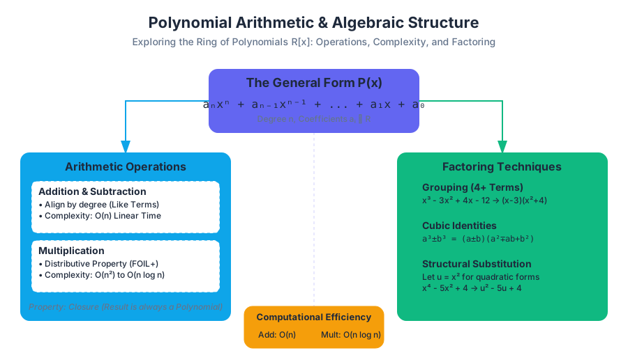
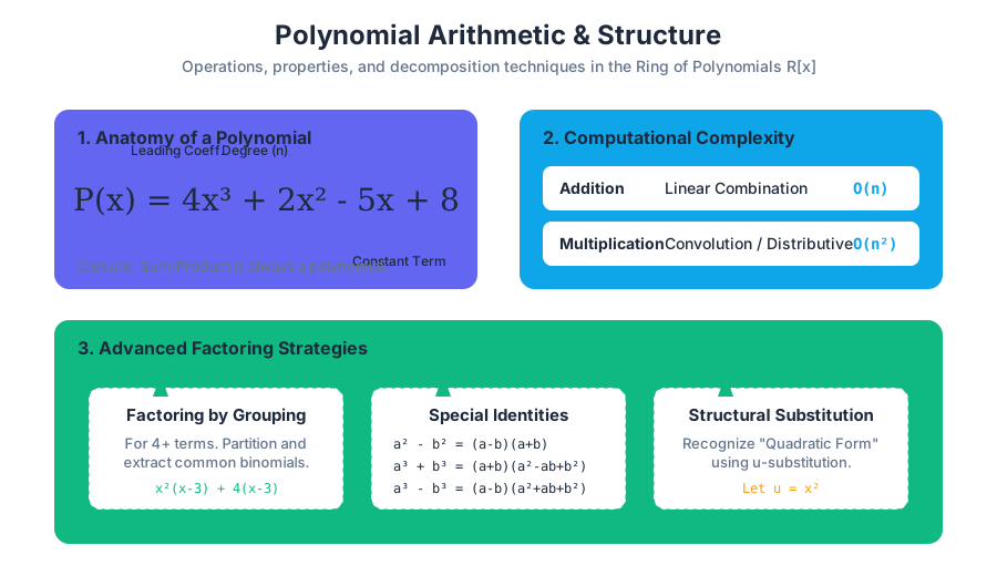
Advanced Functions and Composition

In the foundational study of algebra, functions are often presented as monolithic entities—a single rule applied to a single input to produce a single output. However, as we transition into higher-level mathematics and engineering, we encounter systems that require more nuance. Real-world phenomena rarely follow a single linear or quadratic trajectory across their entire existence. Instead, they are modular, conditional, and interconnected.

This section delves into the sophisticated architecture of functions. We will explore Piecewise Functions, which allow for conditional logic within a mathematical model; Absolute Value Transformations, which introduce symmetry and non-differentiable "corners"; and Function Composition, the process of chaining operations where the output of one system becomes the raw material for the next. Finally, we will establish the rigorous criteria for Inverses, using composition as the ultimate tool for verification.

Piecewise Functions: Modeling Discontinuity and Conditions

A Piecewise Function is a function defined by multiple sub-functions, each applying to a specific interval of the main function's domain. Mathematically, it is expressed using a large brace to group the various "pieces" and their corresponding constraints.

Definition: A function $f(x)$ is piecewise if: $$f(x) = \begin{cases} g_1(x) & \text{if } x \in D_1 \ g_2(x) & \text{if } x \in D_2 \ \vdots & \vdots \ g_n(x) & \text{if } x \in D_n \end{cases}$$ where $D_1, D_2, \dots, D_n$ are disjoint subsets of the domain.

Why Piecewise Functions Matter

In engineering and economics, piecewise functions are the standard for modeling "threshold" behavior. A classic example is the progressive income tax system, where different tax rates apply only to specific "brackets" of income. Similarly, in physics, the force applied by a spring might be linear (Hooke's Law) until it reaches a point of plastic deformation, at which point the governing equation changes entirely.

Mechanics of Evaluation and Graphing

To evaluate a piecewise function at $x = a$, one must first identify which interval $D_i$ contains $a$, and then apply only the rule associated with that interval.

When graphing, the most critical aspect is handling the boundaries (the "fences"). We use:

• Closed circles (●) for inclusive boundaries ($\le$ or $\ge$).
• Open circles (○) for exclusive boundaries ($<$ or $>$).

Feature	Description	Visual Representation
Sub-domain	The specific $x$-range for a rule.	$x < 2$ or $[5, \infty)$
Jump Discontinuity	A gap where the function "jumps" from one value to another.	Vertical break in the graph
Point Discontinuity	A single "hole" in an otherwise continuous line.	An open circle at a specific $(x, y)$
Continuity	When the pieces meet exactly at the boundary.	$g_1(k) = g_2(k)$

Worked Example: The Shipping Cost Algorithm

Consider a logistics company that charges based on weight $w$:

• $5 flat rate for weights up to 2kg.
• $2 per kg for weights between 2kg and 10kg.
• $1.50 per kg plus a $5 heavy-handling fee for weights over 10kg.

def calculate_shipping(weight):
    """
    Implementation of a piecewise shipping cost function.
    Domain: weight > 0
    """
    if weight <= 0:
        raise ValueError("Weight must be positive.")
    
    # Piece 1: Constant flat rate
    if 0 < weight <= 2:
        cost = 5.00
    # Piece 2: Linear rate
    elif 2 < weight <= 10:
        cost = 2.00 * weight
    # Piece 3: Discounted rate with handling fee
    else:
        cost = (1.50 * weight) + 5.00
        
    return round(cost, 2)

# Example usage
print(f"Cost for 1.5kg: ${calculate_shipping(1.5)}") # Output: $5.0
print(f"Cost for 5kg: ${calculate_shipping(5)}")     # Output: $10.0
print(f"Cost for 12kg: ${calculate_shipping(12)}")   # Output: $23.0

Absolute Value Transformations

The absolute value function, $f(x) = |x|$, is technically the simplest piecewise function: $$|x| = \begin{cases} x & \text{if } x \ge 0 \ -x & \text{if } x < 0 \end{cases}$$ However, its transformations are so common in algebra that they are studied as a distinct class of "V-shaped" functions.

The General Form

The standard transformation model for absolute value is: $$g(x) = a|x - h| + k$$

Parameter	Effect	Mathematical Name
$a$	Changes the "steepness" or flips the V upside down.	Vertical Stretch/Compression & Reflection
$h$	Shifts the vertex left or right.	Horizontal Translation
$k$	Shifts the vertex up or down.	Vertical Translation
$(h, k)$	The "tip" of the V.	Vertex

How it Works: The Order of Operations

When graphing $g(x) = -2|x + 3| + 4$, follow the "Inside-Out" rule:

1. Horizontal Shift: Move left by 3 units ($h = -3$).
2. Vertical Stretch/Reflection: Multiply all $y$-values by $-2$. This makes the V narrower and points it downward.
3. Vertical Shift: Move the entire structure up 4 units ($k = 4$).

Pitfalls in Absolute Value

A common mistake is treating $|x - h|$ as $|x| - |h|$. This is the Triangle Inequality error. For example, $|5 - 3| = 2$, but $|5| - |3| = 2$ is a coincidence; consider $|3 - 5| = 2$, whereas $|3| - |5| = -2$. Absolute value is non-linear; it does not distribute.

Function Composition: The Pipeline Model

Function Composition is the mathematical equivalent of a "pipe" in computing. It is the application of one function to the results of another.

Notation: The composition of $f$ and $g$ is written as $(f \circ g)(x)$, which is read as "$f$ of $g$ of $x$." $$(f \circ g)(x) = f(g(x))$$

The Mechanics of the "Inner" and "Outer"

In the expression $f(g(x))$, $g(x)$ is the inner function and $f(x)$ is the outer function.

1. Input $x$ into $g$.
2. Take the output $g(x)$.
3. Use that output as the input for $f$.

Domain Restrictions: The Hidden Complexity

The domain of $(f \circ g)(x)$ is not simply the domain of the resulting simplified expression. It is restricted by two conditions:

1. $x$ must be in the domain of $g$.
2. $g(x)$ must be in the domain of $f$.

If $g(x) = \sqrt{x}$ and $f(x) = \frac{1}{x-4}$, then $x$ must be $\ge 0$ (for $g$) AND $\sqrt{x}$ cannot be 4 (for $f$). Thus, $x \neq 16$. The domain is $[0, 16) \cup (16, \infty)$.

Comparison: $f(g(x))$ vs $g(f(x))$

Composition is not commutative. The order of operations radically changes the result.

Operation	Definition	Example: $f(x)=x^2, g(x)=x+1$
$f(g(x))$	Apply $g$ then $f$	$(x+1)^2 = x^2 + 2x + 1$
$g(f(x))$	Apply $f$ then $g$	$(x^2) + 1 = x^2 + 1$
$f(f(x))$	Self-composition	$(x^2)^2 = x^4$

Mathematical Derivation: Composing Rational Functions

Let $f(x) = \frac{2}{x-1}$ and $g(x) = \frac{3}{x}$. Find $(f \circ g)(x)$.

(f \circ g)(x) = f(g(x))
= f\left(\frac{3}{x}\right)
= \frac{2}{\left(\frac{3}{x}\right) - 1}
= \frac{2}{\frac{3-x}{x}}
= \frac{2x}{3-x}

Domain constraints: $x \neq 0$ (from $g$) and $x \neq 3$ (from the final denominator).

Verifying Inverses through Composition

The most rigorous way to prove that two functions are inverses of each other is through the Inverse Function Property.

The Inverse Theorem: Two functions $f$ and $g$ are inverses if and only if:

1. $f(g(x)) = x$ for all $x$ in the domain of $g$.
2. $g(f(x)) = x$ for all $x$ in the domain of $f$.

If both compositions collapse into the Identity Function $I(x) = x$, the functions effectively "undo" each other.

The Horizontal Line Test

Before seeking an inverse, a function must be one-to-one (injective). If any horizontal line crosses the graph of $f(x)$ more than once, $f(x)$ does not have an inverse function (unless the domain is restricted). For example, $f(x) = x^2$ fails the horizontal line test, but $f(x) = x^2$ for $x \ge 0$ passes.

Step-by-Step Verification

To verify if $f(x) = \frac{x-3}{2}$ and $g(x) = 2x + 3$ are inverses:

1. Compute $f(g(x))$: $f(2x + 3) = \frac{(2x + 3) - 3}{2} = \frac{2x}{2} = x$
2. Compute $g(f(x))$: $g(\frac{x-3}{2}) = 2(\frac{x-3}{2}) + 3 = (x - 3) + 3 = x$
3. Conclusion: Since both equal $x$, they are inverses.

Common Inverse Pairs

Function $f(x)$	Inverse $f^{-1}(x)$	Domain Restriction
$x^n$	$\sqrt[n]{x}$	$x \ge 0$ if $n$ is even
$e^x$	$\ln(x)$	$x > 0$ for $\ln(x)$
$\frac{1}{x}$	$\frac{1}{x}$	$x \neq 0$ (Self-inverse)
$ax + b$	$\frac{x-b}{a}$	$a \neq 0$

Real-World Application: Functional Programming and Data Pipelines

In modern software engineering, the concepts of composition and inverses are used to build robust data pipelines. In functional programming (languages like Haskell, Scala, or Elixir), "composition" is a first-class citizen.

Example: Data Transformation Pipeline

Imagine a system that takes raw user input (string), trims whitespace, converts it to an integer, and then calculates the tax.

// Individual functions (the "pieces")
const trim = (str) => str.trim();
const toInt = (str) => parseInt(str, 10);
const addTax = (num) => num * 1.15;

// Composition: addTax(toInt(trim(input)))
const processPayment = (input) => addTax(toInt(trim(input)));

// Usage
const rawInput = "   100   ";
const finalPrice = processPayment(rawInput); 
console.log(`Final Price: ${finalPrice}`); // Output: 115

This is a direct application of $(f \circ g \circ h)(x)$. If we needed to reverse this process (e.g., to find the original input from the final price), we would need the inverse of each step in reverse order: $h^{-1}(g^{-1}(f^{-1}(y)))$.

Common Pitfalls and Advanced Nuances

1. The "Inverse" vs. "Reciprocal" Confusion: Students often confuse $f^{-1}(x)$ with $\frac{1}{f(x)}$.

   • $f^{-1}(x)$ is the inverse function (undoes the operation).
   • $[f(x)]^{-1}$ is the reciprocal (multiplicative inverse).
   • Example: If $f(x) = x+3$, then $f^{-1}(x) = x-3$, but $[f(x)]^{-1} = \frac{1}{x+3}$.

2. Piecewise Continuity: When designing piecewise functions, ensure the boundaries are defined. If $f(x)$ is defined for $x < 2$ and $x > 2$, the function is undefined at $x=2$. This creates a "hole" in the domain.

3. Composition Order: In $f(g(x))$, always work from the inside out. Evaluating the outer function first is a recipe for algebraic disaster.

4. Absolute Value and Square Roots: Remember that $\sqrt{x^2} = |x|$, not just $x$. This is a fundamental identity that links power functions, radicals, and absolute value.

Study Guide: Advanced Functions

Piecewise Functions

• Definition: Functions with different rules for different domain intervals.
• Key Task: Identify the correct interval before evaluating.
• Graphing: Pay attention to open vs. closed circles at boundaries.

Absolute Value Transformations

• Form: $y = a|x-h|+k$.
• Vertex: Located at $(h, k)$.
• Symmetry: The graph is symmetric about the vertical line $x=h$.

Function Composition

• Notation: $(f \circ g)(x) = f(g(x))$.
• Order: Order matters! $f(g(x)) \neq g(f(x))$ in most cases.
• Domain: The input must survive the inner function AND the resulting output must be valid for the outer function.

Inverses

• Verification: $f(g(x)) = x$ AND $g(f(x)) = x$.
• Existence: Only one-to-one functions have inverses (Horizontal Line Test).
• Graphing: $f(x)$ and $f^{-1}(x)$ are reflections across the line $y=x$.

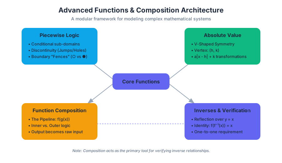
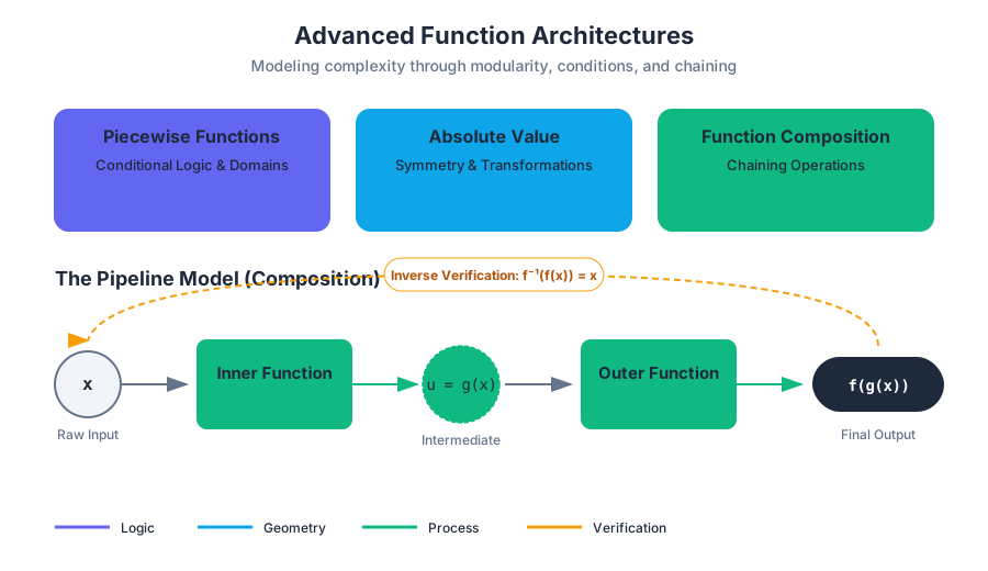
Function Transformations

In the study of calculus and advanced algebra, Function Transformation refers to the process of modifying an existing "parent function" to produce a new, related function. Rather than treating every equation as a unique entity, we view functions as dynamic objects that can be moved, flipped, and Resized within a coordinate plane. This operator-based approach is fundamental to signal processing, computer graphics, and data modeling, where "raw" data must often be normalized or shifted to fit a specific model.

The General Transformation Model

To understand transformations deeply, we must look at the generalized form of a transformed function $g(x)$ based on a parent function $f(x)$:

The Transformation Template: $$g(x) = a \cdot f(b(x - h)) + k$$

In this model, the parameters $(a, b, h, k)$ dictate exactly how the parent graph is altered. These parameters are categorized into External Transformations (affecting the output/y-axis) and Internal Transformations (affecting the input/x-axis).

Parameter	Type	Action	Direction
$k$	External	Vertical Translation	Up if $k > 0$, Down if $k < 0$
$h$	Internal	Horizontal Translation	Right if $h > 0$, Left if $h < 0$
$a$	External	Vertical Dilation/Reflection	Stretch if $
$b$	Internal	Horizontal Dilation/Reflection	Compress if $

---

Translations (Shifting)

A Translation is a rigid transformation that slides the graph of a function without changing its shape, size, or orientation.

Vertical Shifting

A vertical shift occurs when a constant $k$ is added to the output of the function: $g(x) = f(x) + k$. This is an external change. If you add 5 to the entire function, every $y$-value increases by 5, moving the graph up.

Horizontal Shifting

A horizontal shift occurs when a constant $h$ is subtracted from the input: $g(x) = f(x - h)$. The Counter-Intuitive Principle: Students often find horizontal shifts confusing because $f(x - 3)$ moves the graph to the right, while $f(x + 3)$ moves it to the left.

Reasoning: Consider $f(x) = x^2$. To get the output $0$, you need $x=0$. In $g(x) = (x-3)^2$, to get that same output of $0$, $x$ must now be $3$. Therefore, the "origin" of the function has migrated from $0$ to $3$ on the x-axis.

---

Reflections (Flipping)

Reflections are transformations that "flip" the graph across an axis. This is mathematically equivalent to multiplying the input or output by $-1$.

Reflection across the X-axis

When we negate the entire function, $g(x) = -f(x)$, we are negating every $y$-coordinate. This results in a vertical flip across the x-axis.

• Example: $f(x) = \sqrt{x}$ exists only in Quadrant I. $g(x) = -\sqrt{x}$ exists in Quadrant IV.

Reflection across the Y-axis

When we negate only the input, $g(x) = f(-x)$, we are negating every $x$-coordinate. This results in a horizontal flip across the y-axis.

• Example: $f(x) = e^x$ (exponential growth) becomes $g(x) = e^{-x}$ (exponential decay).

Transformation	Equation	Axis of Reflection	Point Mapping
Vertical Reflection	$y = -f(x)$	x-axis	$(x, y) \to (x, -y)$
Horizontal Reflection	$y = f(-x)$	y-axis	$(x, y) \to (-x, y)$

---

Dilations (Scaling)

Dilations are non-rigid transformations that stretch or compress the graph. Unlike translations, dilations change the "slope" or "steepness" of the parent function.

Vertical Scaling ($a$)

The multiplier $a$ in $a \cdot f(x)$ scales the output.

• If $|a| > 1$, the graph undergoes a Vertical Stretch. The function grows faster.
• If $0 < |a| < 1$, the graph undergoes a Vertical Compression. The function grows slower.

Horizontal Scaling ($b$)

The multiplier $b$ in $f(b \cdot x)$ scales the input. This is often the most difficult transformation to visualize because it behaves inversely to the multiplier.

• If $|b| > 1$, the graph undergoes a Horizontal Compression by a factor of $1/b$.
• If $0 < |b| < 1$, the graph undergoes a Horizontal Stretch by a factor of $1/b$.

The Scaling Paradox: In $f(2x)$, the "time" or "space" moves twice as fast, meaning the function completes its behavior in half the distance. Thus, a multiplier of 2 results in a compression to 50% of the original width.

Implementation Example (Numerical Analysis)

In computational science, we often apply these transformations to discrete data arrays. The following Python snippet demonstrates how to apply a transformation pipeline to a NumPy array representing a function.

import numpy as np

def transform_function(x_array, y_array, a=1, b=1, h=0, k=0):
    """
    Applies g(x) = a * f(b(x - h)) + k to discrete data.
    Note: To visualize the transformation on a fixed grid, 
    we manipulate the coordinates.
    """
    # 1. Apply horizontal scaling and shifting to the domain
    # To see the effect of f(b(x-h)), we transform the x-coordinates
    transformed_x = (x_array / b) + h
    
    # 2. Apply vertical scaling and shifting to the codomain
    transformed_y = (a * y_array) + k
    
    return transformed_x, transformed_y

# Example: Parent function f(x) = x^2
x = np.linspace(-10, 10, 100)
y = x**2

# Transform: g(x) = 2 * (0.5(x - 3))^2 + 5
# a=2 (stretch), b=0.5 (horiz stretch), h=3 (right), k=5 (up)
new_x, new_y = transform_function(x, y, a=2, b=0.5, h=3, k=5)

---

Even and Odd Functions (Symmetry)

Symmetry is a specialized property of functions that describes how they behave under reflection. Identifying symmetry allows mathematicians to simplify integrals and engineers to reduce data storage requirements.

Even Functions

A function is Even if it is symmetric about the y-axis. Mathematically, reflecting the function across the y-axis leaves it unchanged.

Algebraic Definition: $f(-x) = f(x)$ for all $x$ in the domain.

• Geometric Insight: If the point $(x, y)$ is on the graph, then $(-x, y)$ must also be on the graph.
• Common Examples: $x^2, x^4, \cos(x), |x|$.

Odd Functions

A function is Odd if it has rotational symmetry of $180^\circ$ about the origin. This is equivalent to reflecting the graph across the y-axis AND the x-axis.

Algebraic Definition: $f(-x) = -f(x)$ for all $x$ in the domain.

• Geometric Insight: If the point $(x, y)$ is on the graph, then $(-x, -y)$ must also be on the graph.
• Common Examples: $x, x^3, \sin(x), 1/x$.

Mathematical Derivation of Symmetry

To prove a function's symmetry, we substitute $(-x)$ into the function and simplify.

Case 1: f(x) = 3x^4 - x^2 + 7
f(-x) = 3(-x)^4 - (-x)^2 + 7
f(-x) = 3(x^4) - (x^2) + 7
f(-x) = f(x)  => EVEN

Case 2: f(x) = x^3 + x
f(-x) = (-x)^3 + (-x)
f(-x) = -x^3 - x
f(-x) = -(x^3 + x)
f(-x) = -f(x) => ODD

Property	Even Functions	Odd Functions
Symmetry	y-axis (Reflection)	Origin (Rotation)
Algebraic Test	$f(-x) = f(x)$	$f(-x) = -f(x)$
Polynomial Powers	All exponents are even	All exponents are odd
Product Rule	Even $\times$ Even = Even	Odd $\times$ Odd = Even
Mixed Rule	Even $\times$ Odd = Odd	Even $+$ Odd = Neither

---

The Order of Operations in Transformations

When multiple transformations are applied simultaneously, the order in which they are performed is critical. Performing a shift before a stretch yields a different result than a stretch before a shift.

The standard convention follows the logic of "Inside-Out" (Horizontal then Vertical) or follows the algebraic order of operations (PEMDAS).

The "B-H" Pitfall

Consider the function $g(x) = f(2x - 6)$. Many students incorrectly identify this as a horizontal compression by 2 and a shift right by 6. However, the horizontal shift $h$ is only apparent when the $b$ value is factored out: $$g(x) = f(2(x - 3))$$ This reveals the true shift is only 3 units to the right.

Recommended Transformation Sequence:

1. Horizontal Shift ($h$)
2. Horizontal Stretch/Compression ($b$)
3. Reflections (if $a$ or $b$ are negative)
4. Vertical Stretch/Compression ($a$)
5. Vertical Shift ($k$)

Pro-Tip: If you follow the form $a \cdot f(b(x - h)) + k$, you can apply all horizontal changes (inside the parentheses) and then all vertical changes (outside).

Real-World Usage: CSS Transforms

In web development, the transform property uses these exact mathematical principles to manipulate DOM elements.

/* 
   Applying transformations to a UI element.
   Note: CSS transforms are applied from right to left in the string.
*/
.hero-image {
  /* 
     1. Scale by 1.5 (Dilation)
     2. Rotate 45deg (Complex transformation)
     3. Translate (Shift) 50px right, 100px down
  */
  transform: translate(50px, 100px) rotate(45deg) scale(1.5);
  
  /* Transition for smooth animation */
  transition: transform 0.3s ease-in-out;
}

.hero-image:hover {
  /* Reflection across the Y-axis using scaleX(-1) */
  transform: translate(50px, 100px) rotate(45deg) scaleX(-1) scaleY(1.5);
}

---

Concrete Example: Transforming the Absolute Value Function

Let's apply a complex transformation to the parent function $f(x) = |x|$. Target Function: $g(x) = -2|x + 4| + 3$

Step-by-Step Breakdown:

1. Parent: Start with $f(x) = |x|$, the V-shape with vertex at $(0,0)$.
2. Horizontal Shift ($h = -4$): Replace $x$ with $x + 4$. The vertex moves to $(-4, 0)$.
3. Vertical Stretch ($a = 2$): Multiply the output by 2. The V-shape becomes narrower (steeper slopes of $\pm 2$).
4. Vertical Reflection ($a$ is negative): Flip the graph over the x-axis. The V-shape now opens downward.
5. Vertical Shift ($k = 3$): Add 3 to the entire function. The vertex moves from $(-4, 0)$ to $(-4, 3)$.

Resulting Vertex: $(-4, 3)$ Domain: $(-\infty, \infty)$ Range: $(-\infty, 3]$

---

Common Pitfalls and Edge Cases

• Ignoring the $b$ Factor: As mentioned, $f(3x - 9)$ is a shift of 3, not 9. Always factor the coefficient of $x$.
• Confusing $a$ and $b$ Effects: Remember that $a$ (vertical) acts "normally" (2 is a stretch, 0.5 is a compression), while $b$ (horizontal) acts "inversely" (2 is a compression, 0.5 is a stretch).
• Symmetry Misconception: Not every function is even or odd. Most functions (like $f(x) = x^2 + x$) are neither. A function must satisfy the algebraic identity perfectly to be classified.
• The Negative Sign: In $f(x-h)$, the formula itself has a negative. So $f(x-5)$ means $h=5$ (positive/right), but $f(x+5)$ means $h=-5$ (negative/left).

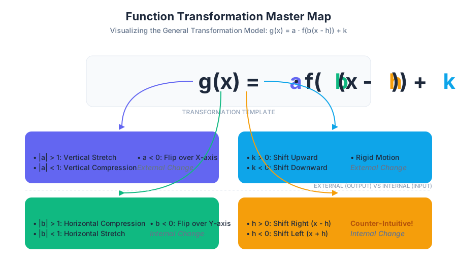
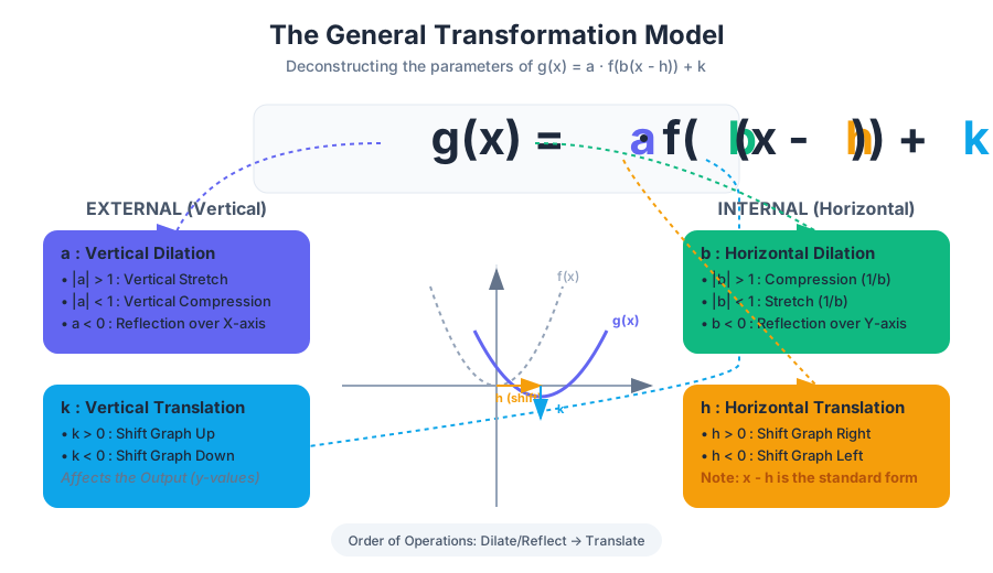
Rational Exponents and Radicals

In the classical study of arithmetic, exponents are often introduced as "repeated multiplication." While this definition suffices for positive integers, it fails to capture the continuous nature of growth and the inverse operations required for modern engineering and physics. The transition from integer exponents to rational exponents represents a fundamental shift in algebraic thinking: the unification of powers and roots into a single, cohesive notation.

By treating roots as fractional powers, we unlock the ability to apply the laws of exponents to radical expressions, simplifying complex calculations and enabling the modeling of phenomena ranging from the orbital mechanics of satellites to the carbon dating of ancient artifacts.

The Mechanics of Rational Exponents

A rational exponent is an exponent expressed as a fraction $m/n$, where $m$ is an integer and $n$ is a positive integer. This notation serves as a bridge between the world of polynomial powers and the world of radicals.

Definition: The Rational Exponent Theorem For any real number $a$ and integers $m$ and $n$ (where $n > 0$), the expression $a^{m/n}$ is defined as: $$a^{m/n} = \sqrt[n]{a^m} = (\sqrt[n]{a})^m$$ This holds true provided that $\sqrt[n]{a}$ is a real number. If $n$ is even and $a < 0$, the result enters the domain of complex numbers.

Why Rational Notation Prevails

In higher-level mathematics and computational science, radical symbols ($\sqrt{\cdot}$) are often discarded in favor of rational exponents. This is not merely a stylistic choice; rational exponents allow for the direct application of the Laws of Exponents, which are far more efficient for symbolic manipulation than radical rules.

Property Name	Radical Notation	Rational Exponent Notation
Product Rule	$\sqrt[n]{a} \cdot \sqrt[n]{b} = \sqrt[n]{ab}$	$a^{1/n} \cdot b^{1/n} = (ab)^{1/n}$
Quotient Rule	$\frac{\sqrt[n]{a}}{\sqrt[n]{b}} = \sqrt[n]{\frac{a}{b}}$	$\frac{a^{1/n}}{b^{1/n}} = (\frac{a}{b})^{1/n}$
Power of a Power	$\sqrt[m]{\sqrt[n]{a}} = \sqrt[mn]{a}$	$(a^{1/n})^{1/m} = a^{1/mn}$
Negative Exponent	$1 / \sqrt[n]{a}$	$a^{-1/n}$

Implementation in Computational Systems

When implementing these concepts in software, particularly for scientific computing, we rely on the power function rather than explicit root functions to maintain precision and handle arbitrary rational scales.

import math

def calculate_rational_exponent(base, numerator, denominator):
    """
    Calculates a^{m/n} using high-precision floating point math.
    Handles the principal root for real numbers.
    """
    try:
        # Standard approach: (base^numerator)^(1/denominator)
        # Note: math.pow handles float exponents natively
        exponent = numerator / denominator
        
        # Check for negative base with even denominator (Complex territory)
        if base < 0 and denominator % 2 == 0:
            return complex(base)**exponent
            
        return math.pow(base, exponent)
    except ValueError as e:
        return f"Domain Error: {e}"

# Example: 32^(2/5) -> (5th root of 32)^2 -> 2^2 = 4
print(f"32^(2/5) = {calculate_rational_exponent(32, 2, 5)}")

Radical Equations and the Isolation Method

A radical equation is an equation in which a variable is contained within a radicand. Solving these equations requires "undoing" the radical by raising both sides of the equation to the power of the index.

The Solving Pipeline

1. Isolate: Move all terms so that one radical expression is alone on one side of the equation.
2. Raise: Raise both sides of the equation to the power equal to the index of the radical (e.g., square both sides for a square root).
3. Linearize/Quadraticize: Solve the resulting polynomial equation.
4. Verify: Check for extraneous solutions, as the squaring process can introduce false roots.

Worked Example: Solving $\sqrt{x + 7} + 5 = x$

Let us solve for $x$ step-by-step.

Step 1: Isolate the radical $$\sqrt{x + 7} = x - 5$$

Step 2: Square both sides $$(\sqrt{x + 7})^2 = (x - 5)^2$$ $$x + 7 = x^2 - 10x + 25$$

Step 3: Set to zero and solve the quadratic $$0 = x^2 - 11x + 18$$ Factoring the quadratic: $$0 = (x - 9)(x - 2)$$ Potential solutions: $x = 9, x = 2$.

Step 4: Check for extraneous solutions

• Test $x = 9$: $\sqrt{9 + 7} + 5 = \sqrt{16} + 5 = 4 + 5 = 9$. (Correct)
• Test $x = 2$: $\sqrt{2 + 7} + 5 = \sqrt{9} + 5 = 3 + 5 = 8 \neq 2$. (Extraneous)

Therefore, the only valid solution is $x = 9$.

\begin{aligned}
&\text{Derivation of the Squaring Property:} \\
&\text{If } a = b, \text{ then } a^n = b^n. \\
&\text{However, if } a^n = b^n, \text{ it does NOT necessarily imply } a = b. \\
&\text{Example: } (-3)^2 = (3)^2 \implies 9 = 9, \text{ but } -3 \neq 3. \\
&\text{This is the fundamental origin of extraneous solutions.}
\end{aligned}

The Phenomenon of Extraneous Solutions

An extraneous solution is a root that emerges during the algebraic manipulation of an equation but does not satisfy the original equation. This typically occurs because the operation of raising to an even power is not injective (one-to-one).

The Geometry of the "False Root"

When we square both sides of $\sqrt{x} = -2$, we get $x = 4$. However, the principal square root of 4 is 2, not -2. Geometrically, squaring a radical equation is equivalent to finding the intersection of a parabola and a line, whereas the original radical equation only represented half of that parabola.

Equation Type	Potential for Extraneous Roots	Reason
Odd Index Roots ($\sqrt[3]{x}$)	Low	$f(x) = x^3$ is a one-to-one mapping; signs are preserved.
Even Index Roots ($\sqrt[2]{x}$)	High	$f(x) = x^2$ maps both $x$ and $-x$ to $x^2$, losing sign information.
Rational Exponents ($x^{2/3}$)	Moderate	Depends on the parity of the numerator and denominator.

Exponential Models and Real-World Scaling

Rational exponents are the engine behind exponential models, which describe systems where the rate of change is proportional to the current value. Unlike linear models, which add a constant amount per unit of time, exponential models multiply by a constant factor.

The General Model

The standard form for exponential growth or decay is: $$A(t) = P(1 + r)^t$$ Where:

• $P$ is the initial amount.
• $r$ is the rate of growth (positive) or decay (negative).
• $t$ is time, which can be a rational number.

Application: Carbon-14 Dating

Carbon-14 has a half-life of approximately 5,730 years. The amount of C-14 remaining after $t$ years is modeled by: $$N(t) = N_0 \cdot (1/2)^{t/5730}$$ Here, the exponent $t/5730$ is a rational number. If we find an artifact with 70% of its original C-14, we solve for $t$ using the properties of exponents and logarithms.

Comparison of Exponential Applications

Field	Model Type	Variable Usage
Finance	Compound Interest	$A = P(1 + r/n)^{nt}$ (Rational exponents via $n$)
Biology	Bacterial Growth	$P = P_0 \cdot 2^{t/d}$ (Doubling time $d$)
Physics	Newton's Law of Cooling	$T(t) = T_a + (T_0 - T_a)e^{-kt}$
Chemistry	Radioactive Decay	$M = M_0 \cdot (1/2)^{t/h}$ (Half-life $h$)

Real-World Usage Example: Financial Modeling

In quantitative finance, we often need to calculate the "Effective Annual Rate" (EAR) when interest is compounded more than once a year. This requires using rational exponents to normalize the time period.

# Using a CLI tool (like 'bc' or a custom python script) to calculate 
# the value of $1000 at 5% interest compounded monthly for 2.5 years.

# Formula: 1000 * (1 + 0.05/12)^(12 * 2.5)
# Note the rational exponent: 30/1 (integer here, but often fractional in day-counts)

python3 -c "print(1000 * (1 + 0.05/12)**(12 * 2.5))"

# Output: 1132.7077...

Advanced Simplification: Rationalizing the Denominator

When working with radicals, it is standard practice to rationalize the denominator, ensuring that no radical remains in the bottom of a fraction. This is particularly important in the pre-calculator era for manual division, but it remains vital today for identifying "like terms" in complex expressions.

The Conjugate Method

To rationalize a binomial denominator involving square roots, we multiply the numerator and denominator by the conjugate. The conjugate of $(a + \sqrt{b})$ is $(a - \sqrt{b})$.

Example: Simplify $\frac{3}{5 - \sqrt{2}}$ $$\frac{3}{5 - \sqrt{2}} \cdot \frac{5 + \sqrt{2}}{5 + \sqrt{2}} = \frac{3(5 + \sqrt{2})}{25 - 2} = \frac{15 + 3\sqrt{2}}{23}$$

Pitfalls in Simplification

A common error occurs when students attempt to distribute a root over addition: $$\sqrt{a^2 + b^2} \neq a + b$$ This is a violation of the order of operations. Exponents (and radicals) do not distribute over addition or subtraction.

Correct Operation	Incorrect Operation
$(ab)^{1/2} = a^{1/2}b^{1/2}$	$(a+b)^{1/2} = a^{1/2} + b^{1/2}$ (FALSE)
$\sqrt{x^2} = \vert x\vert $	$\sqrt{x^2} = x$ (Only true if $x \geq 0$)
$x^{a} \cdot x^{b} = x^{a+b}$	$x^{a} \cdot x^{b} = x^{ab}$ (FALSE)

Performance and Edge Cases in Computation

When dealing with very large exponents or very small roots in a computational context, we encounter the limits of floating-point representation.

1. Precision Loss: Calculating $x^{1/n}$ for large $n$ can result in values extremely close to 1, leading to "catastrophic cancellation" in subsequent subtractions.
2. Negative Bases: As mentioned, $(-8)^{1/3} = -2$ is well-defined in real numbers, but $(-8)^{1/2}$ is $2i$. Most standard libraries (like Python's math) will throw a ValueError for the latter, requiring the use of complex number modules (cmath).
3. The Principal Root: Mathematically, $x^2 = 4$ has two solutions ($2, -2$). However, the function $f(x) = x^{1/2}$ is defined only as the principal root (positive). Software must strictly adhere to this to remain functional.

import cmath

# Edge Case: Negative base with fractional exponent
base = -8
exponent = 1/3

# Standard math fails on negative bases for fractional powers
# cmath handles the complex plane correctly
result = cmath.exp(exponent * cmath.log(base))

print(f"The complex principal root of {base}^{exponent:.2f} is {result}")
# Note: This may return a complex number even if a real root exists 
# due to how cmath defines the principal branch.

Summary of Best Practices

To master rational exponents and radicals, one must treat the radical symbol as a mere "costume" for a fraction. By converting all radicals to rational exponents at the start of a problem, the rules of algebra become uniform.

• Always check for extraneous solutions when you have raised both sides of an equation to an even power.
• Isolate the most complex radical first before squaring.
• Use conjugates to clear radicals from denominators.
• Remember the absolute value when simplifying $\sqrt[n]{x^n}$ for even $n$.

Logarithms: The Calculus of Proportions and Inverses

Logarithms are the inverse operation of exponentiation. While an exponent asks, "What do I get when I raise this base to this power?", a logarithm asks, "To what power must I raise this base to reach this specific value?" This shift in perspective—from the result of growth to the duration or intensity of growth—is what makes logarithms the fundamental language of the natural sciences, finance, and information theory.

The Anatomy of a Logarithm

At its core, a logarithm is a functional relationship. If we have an exponential equation $b^y = x$, the logarithmic equivalent is written as:

$$\log_b(x) = y$$

Where:

• $b$ is the base (the number being multiplied).
• $x$ is the argument (the value we wish to reach).
• $y$ is the exponent (the power to which the base is raised).

The Fundamental Identity: For any valid base $b$, $b^{\log_b(x)} = x$ and $\log_b(b^x) = x$. This confirms that logarithms and exponentials "undo" each other.

Constraints and Domains

Logarithms are not defined for all real numbers. Because a positive base $b$ raised to any real power $y$ will always yield a positive result $x$, the following constraints apply:

1. The base $b$ must be positive ($b > 0$).
2. The base $b$ cannot be 1 ($b \neq 1$), as $1^y$ is always 1.
3. The argument $x$ must be positive ($x > 0$). Logarithms of negative numbers or zero are undefined in the real number system.

Component	Notation	Domain/Constraint	Role in Growth
Base	$b$	$b \in (0, 1) \cup (1, \infty)$	The constant factor of multiplication.
Argument	$x$	$x \in (0, \infty)$	The target value or "total growth."
Logarithm	$y$	$y \in (-\infty, \infty)$	The "time" or "scaling factor" required.

Fundamental Properties and Derivations

The power of logarithms lies in their ability to transform complex operations into simpler ones. Specifically, they turn multiplication into addition, division into subtraction, and exponentiation into multiplication. These properties are not arbitrary; they are direct consequences of the laws of exponents.

The Product Rule

The logarithm of a product is the sum of the logarithms of its factors: $$\log_b(MN) = \log_b(M) + \log_b(N)$$

Derivation: Let $x = \log_b(M)$ and $y = \log_b(N)$. By definition, $b^x = M$ and $b^y = N$. Multiplying the two: $M \cdot N = b^x \cdot b^y = b^{x+y}$. Converting back to logarithmic form: $\log_b(MN) = x + y$. Substituting back: $\log_b(MN) = \log_b(M) + \log_b(N)$.

The Quotient Rule

The logarithm of a quotient is the difference of the logarithms: $$\log_b\left(\frac{M}{N}\right) = \log_b(M) - \log_b(N)$$

The Power Rule

The logarithm of a number raised to an exponent is the exponent multiplied by the logarithm of the number: $$\log_b(M^p) = p \cdot \log_b(M)$$

Summary of Operational Transformations

Exponential Operation	Logarithmic Equivalent	Transformation Type
$b^x \cdot b^y$	$\log(M) + \log(N)$	Linearization (Add)
$b^x / b^y$	$\log(M) - \log(N)$	Linearization (Subtract)
$(b^x)^y$	$y \cdot \log(M)$	Reduction (Multiply)
$\sqrt[y]{b^x}$	$\frac{1}{y} \cdot \log(M)$	Reduction (Divide)

The Change of Base Formula

Historically, mathematicians and engineers relied on printed tables for $\log_{10}$ (Common Log) and $\ln$ (Natural Log, base $e$). If a problem required $\log_2$ or $\log_7$, they needed a way to convert between bases. This is achieved via the Change of Base Formula:

$$\log_b(a) = \frac{\log_c(a)}{\log_c(b)}$$

Where $c$ is any new base you choose (typically $10$ or $e$).

Why it matters in Computing

Most programming languages provide standard functions for the natural logarithm (log() or ln()) and sometimes base 10 (log10()). To calculate a custom base, the Change of Base formula is the standard implementation path.

import math

def log_custom_base(value, base):
    """
    Calculates log of 'value' with 'base' using the 
    Change of Base formula: log_b(a) = ln(a) / ln(b)
    """
    if value <= 0:
        raise ValueError("Logarithm argument must be positive.")
    if base <= 0 or base == 1:
        raise ValueError("Logarithm base must be positive and not equal to 1.")
    
    # Using math.log which defaults to base e (natural log)
    return math.log(value) / math.log(base)

# Example: Evaluating log base 2 of 1024
result = log_custom_base(1024, 2)
print(f"log2(1024) = {result}") # Output: 10.0

Evaluating Logarithms and Solving Equations

Solving logarithmic equations generally follows two strategies: Isolating the Logarithm or Exponentiating both sides.

Strategy 1: Converting to Exponential Form

When faced with $\log_2(x-3) = 4$, we rewrite the equation: $2^4 = x - 3$ $16 = x - 3$ $x = 19$

Strategy 2: Using One-to-One Property

If $\log_b(M) = \log_b(N)$, then $M = N$. Example: $\log(2x + 1) = \log(x + 5)$ $2x + 1 = x + 5$ $x = 4$

Strategy 3: Solving for Exponents (The "Log Both Sides" Method)

This is the primary method for solving equations like $5^x = 12$.

1. Take the log of both sides: $\log(5^x) = \log(12)$
2. Apply the Power Rule: $x \cdot \log(5) = \log(12)$
3. Isolate $x$: $x = \frac{\log(12)}{\log(5)} \approx 1.544$

Exponential Word Problems and Real-World Applications

Logarithms are essential for modeling phenomena where the rate of change depends on the current value. These are often categorized into Growth, Decay, and Intensity Scales.

1. Compound Interest and Population Growth

The formula for continuous growth is $A = Pe^{rt}$. To find the time $t$ it takes for an investment to double: $2P = Pe^{rt}$ $2 = e^{rt}$ $\ln(2) = rt$ $t = \frac{\ln(2)}{r}$

2. The Richter Scale (Earthquakes)

The magnitude $M$ of an earthquake is a logarithmic scale: $M = \log_{10}\left(\frac{I}{S}\right)$ Where $I$ is the intensity and $S$ is a standard threshold. Because it is base 10, a magnitude 7 earthquake is not "one unit" stronger than a magnitude 6; it is 10 times more intense in terms of amplitude and roughly 31.6 times more energetic.

3. pH in Chemistry

The acidity of a solution is defined by the negative logarithm of the hydrogen ion concentration: $\text{pH} = -\log_{10}[H^+]$

4. Decibels (Sound)

Sound intensity is measured relative to the threshold of human hearing: $L_{dB} = 10 \cdot \log_{10}\left(\frac{I}{I_0}\right)$

Application	Base	Dependent Variable	Context
Finance	$e$	Time ($t$)	Continuous compounding interest.
Seismology	$10$	Magnitude ($M$)	Earthquake energy release.
Chemistry	$10$	pH	Acidity/Alkalinity of liquids.
Acoustics	$10$	Decibels ($dB$)	Relative loudness of sound.
Computer Science	$2$	Bits/Complexity	Binary search, entropy, tree depth.

Advanced Implementation: Logarithmic Derivations in Pseudocode

In computational contexts, logarithms are often used to prevent "Arithmetic Underflow." When multiplying many small probabilities (as in Naive Bayes or Hidden Markov Models), the result can become so small that a computer rounds it to zero. By taking the log, we turn these multiplications into additions, preserving precision.

\text{Problem: Calculate } P = \prod_{i=1}^{n} p_i \text{ where } p_i \text{ is very small.}
\text{Solution: } \log(P) = \sum_{i=1}^{n} \log(p_i)
\text{Final Result: } P = \exp(\log(P))

// Pseudocode for Log-Sum-Exp Trick to avoid underflow
function calculate_joint_probability(probabilities[])
    log_sum = 0
    for each p in probabilities:
        if p <= 0:
            return -Infinity // Log of 0 is undefined
        log_sum = log_sum + log(p)
    
    return log_sum // Return in log-space to maintain precision
end function

// Usage in a classifier
log_prob_class_A = calculate_joint_probability(features_A)
log_prob_class_B = calculate_joint_probability(features_B)

if log_prob_class_A > log_prob_class_B:
    print("Class A is more likely")

Common Pitfalls and Edge Cases

1. The Negative Argument Trap: Students often try to solve $\log(x) + \log(x-3) = \log(4)$ and find two solutions, say $x=4$ and $x=-1$. However, $x=-1$ must be discarded because the domain of a logarithm is $(0, \infty)$. Always check for extraneous solutions.
2. Confusing $\log(x+y)$ with $\log(x) + \log(y)$: There is no property for the logarithm of a sum. $\log(x+y)$ cannot be simplified.
3. Base Confusion: In many scientific contexts, log refers to $\ln$ (base $e$), while in engineering, log often refers to $\log_{10}$. In computer science, it frequently implies $\log_2$. Always verify the context's default base.
4. The Power Rule Misapplication: In the expression $(\log_b x)^p$, the power $p$ applies to the entire logarithm, not the argument. Therefore, $p$ cannot be moved to the front. Only in $\log_b(x^p)$ is the power rule applicable.

Real-World Usage: Calculating Half-Life via CLI

In a laboratory setting, a researcher might use a quick shell command to calculate the remaining mass of a radioactive isotope using the decay constant derived from a logarithm.

# Calculate the time required for a substance to decay to 25% 
# given a half-life of 5730 years (Carbon-14).
# Formula: t = [ ln(N/N0) / -k ] where k = ln(2) / half_life

HALF_LIFE=5730
TARGET_RATIO=0.25

# Use 'bc' (basic calculator) with math library (-l)
echo "scale=5; l($TARGET_RATIO) / -(l(2)/$HALF_LIFE)" | bc -l

# Output: 11460.00000 (Exactly two half-lives)

Client Challenge: Final Assessment

The Final Assessment represents the terminal phase of the College Algebra curriculum, a rigorous synthesis of thirteen distinct units of mathematical theory. It is designed not merely as a recall-based examination but as a high-stakes validation of a learner’s Algebraic Mastery. In this context, mastery is defined as the ability to fluidly transition between symbolic manipulation, graphical interpretation, and real-world modeling across linear, non-linear, and transcendental functions.

The Architecture of Cumulative Knowledge

The assessment is structured to evaluate a student's "mathematical maturity." This involves the transition from procedural fluency (knowing how to solve) to conceptual depth (knowing why a method works and when to apply it). The curriculum builds a vertical stack of dependencies, where the failure to master a foundational concept like Linear Intercepts creates a cascading bottleneck when approaching Rational Function Asymptotes.

The Hierarchy of Algebraic Domains

To succeed in the Final Assessment, one must navigate four primary domains of algebraic thought:

Domain	Core Focus	Key Assessment Indicators
Linearity	Constant rates of change	Slope-intercept forms, systems of equations, compound inequalities.
Quadratics	Parabolic motion & optimization	Factoring patterns, vertex forms, complex roots ($i$).
Transcendental	Growth, decay, and scales	Logarithmic properties, exponential modeling, radical simplification.
Structural	Function behavior	Domain/range, inverses, transformations, polynomial arithmetic.

Technical Prerequisite: The JavaScript Execution Layer

A unique aspect of the "Client Challenge" platform is its reliance on client-side scripting. As noted in the technical requirements, the assessment interface is a Dynamic Web Application. Without JavaScript enabled, the Document Object Model (DOM) cannot render the LaTeX-based math symbols or the interactive graphing tools required for the exam.

Access Error Protocol: If a user encounters the "JavaScript is disabled" notification, the cryptographic handshake between the client and the assessment server fails. This is a security and functional measure to ensure that the interactive "Area Models" for binomial multiplication and the "Coordinate Plane" inputs function with sub-millisecond latency.

// Example: Client-side validation for JavaScript readiness in the Assessment Portal
function checkAssessmentReady() {
    const requirements = {
        jsEnabled: true,
        browserWidth: window.innerWidth,
        mathJaxLoaded: typeof MathJax !== 'undefined'
    };

    if (requirements.jsEnabled && requirements.mathJaxLoaded) {
        console.log("Assessment Environment: OPTIMAL");
        document.getElementById('start-btn').disabled = false;
    } else {
        alert("Critical: Please enable JavaScript and allow MathJax to load.");
    }
}

Core Competency Pillars

1. Linear Systems and Absolute Value

The assessment tests the ability to solve multi-step equations where the variable may appear on both sides, often requiring the distribution of constants and the collection of like terms. A significant "trap" in this section involves Absolute Value Equations.

• The Logic: $|ax + b| = c$ implies two distinct paths: $ax + b = c$ and $ax + b = -c$.
• The Pitfall: Forgetting to check for extraneous solutions, especially when the absolute value is set equal to a variable expression (e.g., $|x-3| = 2x$).

2. Quadratic Dynamics and Factoring Mastery

Factoring is the "Swiss Army Knife" of algebra. The Final Assessment evaluates speed and accuracy in identifying which factoring method to deploy.

Pattern Name	Algebraic Form	Application Context
Difference of Squares	$a^2 - b^2 = (a-b)(a+b)$	Simplifying rational expressions.
Perfect Square Trinomial	$a^2 + 2ab + b^2 = (a+b)^2$	Completing the square for vertex form.
Factoring by Grouping	$ax + ay + bx + by$	Solving higher-degree polynomials.
AC Method	$ax^2 + bx + c$	Factoring when the leading coefficient $a \neq 1$.

3. The Complex Number System

The introduction of the imaginary unit $i$, where $i^2 = -1$, expands the assessment's scope into the complex plane. Mastery here requires performing arithmetic on complex numbers and understanding the Complex Conjugate.

Theorem (Conjugate Pair Theorem): If a polynomial has real coefficients and $a + bi$ is a root, then its conjugate $a - bi$ must also be a root.

# Low-level implementation of a Quadratic Solver handling Complex Roots
import cmath

def solve_quadratic(a, b, c):
    """
    Solves ax^2 + bx + c = 0 and returns a tuple of roots.
    Utilizes the cmath library for complex number support.
    """
    # Calculate the discriminant
    d = (b**2) - (4*a*c)

    # Find two solutions
    root1 = (-b - cmath.sqrt(d)) / (2 * a)
    root2 = (-b + cmath.sqrt(d)) / (2 * a)

    return root1, root2

# Example: Solving x^2 + 4x + 5 = 0
# Expected: -2-1j and -2+1j
print(f"Roots: {solve_quadratic(1, 4, 5)}")

Advanced Function Analysis

A major portion of the Final Assessment focuses on Function Transformations and Inverses. Students must visualize how modifying a function's equation shifts its graph.

Transformation Mapping Table

Let $f(x)$ be the parent function. The following table summarizes the effects of constants $h, k,$ and $a$:

Transformation	Notation	Visual Effect
Vertical Shift	$f(x) + k$	Moves graph up/down by $k$ units.
Horizontal Shift	$f(x - h)$	Moves graph left/right by $h$ units (Inverse logic).
Vertical Stretch	$a \cdot f(x)$	Stretches/compresses graph vertically.
Reflection (x-axis)	$-f(x)$	Flips the graph over the x-axis.

Inverse Functions

To find the inverse $f^{-1}(x)$, the assessment requires a two-step algebraic process:

1. Replace $f(x)$ with $y$ and swap $x$ and $y$.
2. Solve the new equation for $y$.

The graphical relationship is a reflection across the line $y = x$. The domain of the original function becomes the range of the inverse, a critical concept for logarithmic functions.

Transcendental Mastery: Exponents and Logarithms

The Final Assessment concludes with the most abstract concepts: Logarithmic and Exponential Functions. These are inverse operations of one another. The assessment tests the laws of logarithms, which are essential for solving equations where the variable is in the exponent.

The Laws of Logarithms (Derivation)

The following identities are the primary tools for "expanding" or "condensing" expressions:

1.  \log_b(xy) = \log_b(x) + \log_b(y)  \quad \text{(Product Rule)}
2.  \log_b(x/y) = \log_b(x) - \log_b(y) \quad \text{(Quotient Rule)}
3.  \log_b(x^p) = p \cdot \log_b(x)       \quad \text{(Power Rule)}
4.  \log_b(x) = \frac{\ln(x)}{\ln(b)}      \quad \text{(Change of Base)}

Worked Example: Solving an Exponential Equation Solve for $x$: $5^{2x-1} = 125$.

1. Recognize Bases: $125$ can be written as $5^3$.
2. Equate Exponents: If $5^{2x-1} = 5^3$, then $2x - 1 = 3$.
3. Solve: $2x = 4 \implies x = 2$.

If the bases were not powers of each other (e.g., $5^x = 17$), the student would need to take the natural log ($\ln$) of both sides and apply the Power Rule.

Exam Patterns and Strategic Heuristics

Senior educators identify three common patterns in the Final Assessment that often trip up students:

1. The "Number of Solutions" Query: Instead of asking for the solution, the exam asks how many solutions exist. For linear equations, this involves checking if the slopes and intercepts are identical (infinite solutions) or if slopes are equal but intercepts differ (no solution).
2. Contextual Interpretation: Problems that provide a 2-variable equation (e.g., $C = 15h + 50$) and ask for the "meaning of the constant 50." In this context, 50 represents the $y$-intercept or the "initial cost."
3. Compound Inequality Boundaries: When solving $-3 < 2x + 1 \leq 7$, the student must perform operations on all three "sides" of the inequality simultaneously.

# Using a CLI tool like 'gnuplot' to visualize function behavior before an exam
# This helps in understanding transformations and intercepts.

gnuplot -e "set terminal png; \
            set output 'transformation.png'; \
            set grid; \
            plot [x=-5:5] x**2 title 'Parent', \
            (x-2)**2 + 3 title 'Shifted (Right 2, Up 3)'"

Conclusion: The Path to Calculus

The Client Challenge: Final Assessment is the gateway to higher-level mathematics. Mastery of these concepts ensures that when a student encounters a derivative in Calculus or a complex vector in Physics, the underlying algebra is "invisible"—a fluent language rather than a series of hurdles. Success requires a blend of technical browser configuration (JavaScript), procedural accuracy (Factoring), and conceptual synthesis (Function Analysis).

• Slope-Intercept Form: $y = mx + b$, where $m$ is slope and $b$ is $y$-intercept.
• Discriminant: The part of the quadratic formula $b^2 - 4ac$ that determines the nature of the roots.
• Extraneous Solution: A solution that emerges from the algebraic process but does not satisfy the original equation (common in radical and rational equations).
• Asymptote: A line that a graph approaches but never touches, common in rational and logarithmic functions.
• Complex Conjugate: For a complex number $a + bi$, the conjugate is $a - bi$. Their product is always a real number ($a^2 + b^2$).
• Logarithm: The exponent to which a base must be raised to produce a given number.

1. Concept: If a system of two linear equations has the same slope but different y-intercepts, how many solutions does it have? (Answer: Zero/No solution).
2. Application: Solve $|2x - 5| = 11$. (Answer: $x = 8$ and $x = -3$).
3. Factoring: What is the first step in factoring $3x^2 - 12$? (Answer: Factor out the Greatest Common Factor, which is 3).
4. Complex Numbers: Simplify $i^{14}$. (Answer: $-1$, because $i^4 = 1$, so $i^{12} = 1$, leaving $i^2$).
5. Logarithms: Convert $\log_2(32) = 5$ into exponential form. (Answer: $2^5 = 32$).
6. Transformations: How does the graph of $g(x) = f(x+4) - 2$ compare to $f(x)$? (Answer: Shifted left 4 units and down 2 units).

Final Assessment Checklist:

• Linearity: Can you find the equation of a line passing through two points using the point-slope formula?
• Systems: Can you solve a $2 \times 2$ system using both substitution and elimination?
• Quadratics: Do you recognize the "Difference of Squares" instantly?
• Functions: Can you identify the domain of a function with a square root (where the radicand must be $\geq 0$)?
• Exponents: Do you remember that $x^{-n} = 1/x^n$?
• Logarithms: Can you use the Change of Base formula to evaluate $\log_3(10)$ on a standard calculator?
• Technical: Is your browser updated and is JavaScript enabled for the interactive graphing portions of the exam?