Chemistry 2e

Foundations of Chemistry: Matter and Measurement

Overview

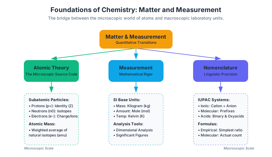
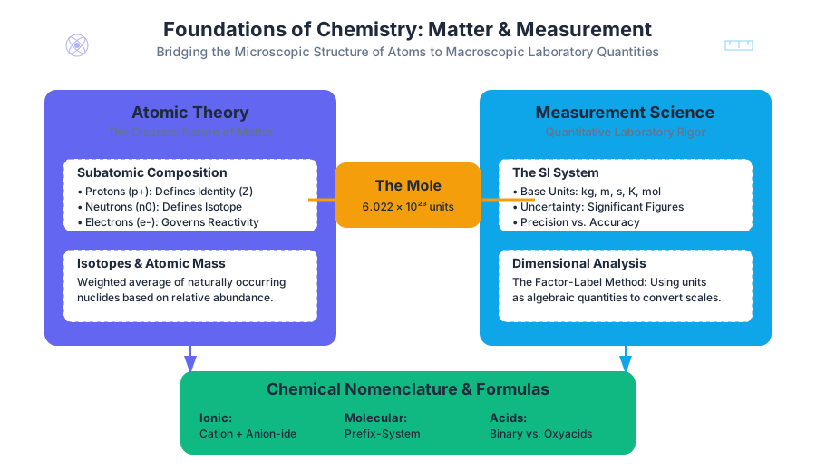
Chemistry is often defined as the study of matter and the changes it undergoes. However, at a more rigorous level, it is the science of quantitative transitions. To understand these transitions, one must master the bridge between the microscopic world of atoms and the macroscopic world of laboratory measurements. This section establishes the fundamental framework of chemistry, integrating the structural logic of Atomic Theory, the linguistic precision of Chemical Nomenclature, and the mathematical rigor of Stoichiometry and Dimensional Analysis.

Atomic Theory: The Discrete Nature of Matter

Modern chemistry rests upon the realization that matter is not continuous, but composed of discrete units called atoms. This concept, first formalized by John Dalton in the early 19th century, provides the "source code" for understanding chemical behavior.

The Evolution of the Atom

While Dalton envisioned atoms as indivisible spheres, modern physics reveals a complex internal structure. The behavior of an element is dictated by its subatomic composition—specifically the arrangement of protons, neutrons, and electrons.

The Law of Definite Proportions: A fundamental chemical principle stating that a given chemical compound always contains its component elements in a fixed ratio (by mass) and does not depend on its source and method of preparation.

Particle	Symbol	Charge (e)	Mass (amu)	Location
Proton	$p^+$	+1	1.00727	Nucleus
Neutron	$n^0$	0	1.00866	Nucleus
Electron	$e^-$	-1	0.00055	Extranuclear

Isotopes and Atomic Mass

The identity of an element is defined solely by its Atomic Number ($Z$), the number of protons. However, atoms of the same element can have different numbers of neutrons, known as Isotopes. The Atomic Mass reported on the periodic table is a weighted average of all naturally occurring isotopes.

# Implementation: Calculating Weighted Average Atomic Mass
# This script simulates the calculation found on the periodic table 
# based on isotopic abundance data.

def calculate_atomic_mass(isotopes):
    """
    isotopes: List of dictionaries containing 'mass' (float) and 'abundance' (float 0-1)
    """
    total_mass = sum(iso['mass'] * iso['abundance'] for iso in isotopes)
    return round(total_mass, 5)

# Example: Magnesium Isotopes
mg_isotopes = [
    {"mass": 23.98504, "abundance": 0.7899}, # Mg-24
    {"mass": 24.98584, "abundance": 0.1000}, # Mg-25
    {"mass": 25.98259, "abundance": 0.1101}  # Mg-26
]

print(f"Calculated Atomic Mass of Mg: {calculate_atomic_mass(mg_isotopes)} amu")
# Output: Calculated Atomic Mass of Mg: 24.30505 amu

Common Pitfalls in Atomic Theory

1. Confusing Mass Number with Atomic Mass: The mass number ($A$) is an integer (protons + neutrons) for a specific isotope, whereas atomic mass is a decimal average.
2. Charge Misconceptions: Ions are formed by the gain or loss of electrons, never protons. Changing the proton count changes the element itself.

---

Measurement and Dimensional Analysis

In chemistry, a number without a unit is meaningless. Dimensional Analysis (or the Factor-Label Method) is the primary tool for navigating the scales of the universe, from picometers to kilometers.

The SI System and Uncertainty

Chemistry utilizes the International System of Units (SI). Because every measurement involves an instrument, every measurement carries Uncertainty. This is expressed through Significant Figures.

Quantity	Base Unit	Symbol	Common Derived Units
Length	Meter	m	cm, nm, Å
Mass	Kilogram	kg	g, mg, μg
Time	Second	s	ms, ns
Temperature	Kelvin	K	Celsius (°C)
Amount	Mole	mol	mmol
Volume	Cubic Meter	$m^3$	Liter (L), mL

Precision vs. Accuracy

• Accuracy: How close a measurement is to the true or accepted value.
• Precision: How close a series of measurements are to one another (reproducibility).

How Dimensional Analysis Works

Dimensional analysis treats units as algebraic quantities that can be cancelled out. This prevents "conversion drift" and ensures that the final answer is physically logical.

// A Rust-inspired conceptual example of Type-Safe Unit Conversion
// Demonstrating how modern systems prevent dimensional errors at compile time.

struct Grams(f64);
struct Moles(f64);
struct MolarMass(f64); // grams per mole

impl Grams {
    fn to_moles(&self, mw: MolarMass) -> Moles {
        Moles(self.0 / mw.0)
    }
}

fn main() {
    let mass = Grams(50.0);
    let mw_h2o = MolarMass(18.015);
    
    let amount = mass.to_moles(mw_h2o);
    
    println!("Moles of H2O: {:.4}", amount.0);
}

---

Chemical Formulas and Nomenclature

A Chemical Formula represents the elemental composition of a substance. Understanding these formulas is the prerequisite for stoichiometry.

Molecular vs. Empirical Formulas

• Empirical Formula: The simplest whole-number ratio of atoms in a compound (e.g., $CH_2O$ for glucose).
• Molecular Formula: The actual number of atoms of each element in a molecule (e.g., $C_6H_{12}O_6$ for glucose).

Nomenclature Systems

Naming follows strict IUPAC (International Union of Pure and Applied Chemistry) conventions.

Compound Type	Naming Rule	Example
Ionic (Type I)	Cation + Anion-ide	$NaCl$ (Sodium Chloride)
Ionic (Type II)	Cation (Roman Numeral) + Anion	$FeCl_3$ (Iron(III) Chloride)
Molecular	Prefix-Element + Prefix-Element-ide	$N_2O_4$ (Dinitrogen Tetroxide)
Acids (Binary)	Hydro-root-ic Acid	$HCl$ (Hydrochloric Acid)
Oxyacids	Root-ic/ous Acid	$H_2SO_4$ (Sulfuric Acid)

---

The Mole and Stoichiometry: The Quantitative Core

Stoichiometry is the calculation of relative quantities of reactants and products in chemical reactions. It is the "accounting" of chemistry.

The Mole Concept

The Mole ($mol$) is the SI unit for amount of substance. It is defined as exactly $6.02214076 \times 10^{23}$ (Avogadro's Number) elementary entities. This number is chosen so that the mass of one mole of a substance in grams is numerically equal to the mass of one atom/molecule in atomic mass units (amu).

Reaction Balancing and Molar Ratios

A balanced chemical equation obeys the Law of Conservation of Mass. The coefficients in a balanced equation represent the Molar Ratio between substances.

\text{The General Stoichiometric Equation:} \\
aA + bB \rightarrow cC + dD \\
\text{Where } a, b, c, d \text{ are stoichiometric coefficients.}

Limiting Reactants and Percent Yield

In real-world scenarios, reactants are rarely present in exact stoichiometric proportions. The Limiting Reactant is the reagent that is entirely consumed first, limiting the amount of product formed.

Theoretical Yield: The maximum amount of product that can be produced from a given amount of limiting reactant. Actual Yield: The amount of product actually obtained from a reaction. Percent Yield: $(\text{Actual Yield} / \text{Theoretical Yield}) \times 100%$.

Concrete Example: Combustion of Propane

Calculate the mass of $CO_2$ produced when 44.1 g of $C_3H_8$ is burned in excess $O_2$.

1. Balanced Equation: $C_3H_8 + 5O_2 \rightarrow 3CO_2 + 4H_2O$
2. Molar Mass of $C_3H_8$: $\approx 44.1 , g/mol$
3. Moles of $C_3H_8$: $44.1 , g / 44.1 , g/mol = 1.00 , mol$
4. Molar Ratio: $1 , mol , C_3H_8 : 3 , mol , CO_2$
5. Moles of $CO_2$: $1.00 , mol \times 3 = 3.00 , mol$
6. Mass of $CO_2$: $3.00 , mol \times 44.01 , g/mol = 132.03 , g$

---

Advanced Stoichiometry: Solution and Gas Phase

Stoichiometry is not limited to solids. In liquid phases, we use Molarity ($M$); in gas phases, we use the Ideal Gas Law.

Molarity and Dilution

Molarity is defined as moles of solute per liter of solution ($mol/L$).

Parameter	Definition	Formula
Molarity (M)	Concentration	$M = \frac{n}{V}$
Dilution	Reducing concentration	$M_1V_1 = M_2V_2$
Mass Percent	Mass ratio	$\frac{\text{mass solute}}{\text{total mass}} \times 100$

Database Schema for Stoichiometric Tracking

In industrial settings (e.g., pharmaceutical manufacturing), stoichiometry is tracked via relational databases to ensure batch consistency and regulatory compliance.

-- Schema for a Chemical Batch Tracking System
CREATE TABLE elements (
    id SERIAL PRIMARY KEY,
    symbol VARCHAR(3) UNIQUE NOT NULL,
    atomic_weight DECIMAL(10, 5) NOT NULL
);

CREATE TABLE compounds (
    id SERIAL PRIMARY KEY,
    formula VARCHAR(50) NOT NULL,
    molecular_weight DECIMAL(10, 5)
);

CREATE TABLE batch_runs (
    batch_id UUID PRIMARY KEY,
    compound_id INTEGER REFERENCES compounds(id),
    theoretical_yield_grams DECIMAL(15, 2),
    actual_yield_grams DECIMAL(15, 2),
    percent_yield DECIMAL(5, 2) GENERATED ALWAYS AS 
        ((actual_yield_grams / theoretical_yield_grams) * 100) STORED
);

---

Variations and Extensions

1. Non-Stoichiometric Compounds

In solid-state chemistry, some compounds (Berthollides) do not have fixed integer ratios (e.g., $Fe_{0.95}O$). These challenge the traditional Daltonian view but are critical in materials science and superconductivity.

2. Green Chemistry Metrics

Modern stoichiometry extends beyond yield to include Atom Economy: $$\text{Atom Economy} = \frac{\text{Mass of Desired Product}}{\text{Total Mass of Reactants}} \times 100$$ High yield does not always mean a "green" process if the byproduct mass is excessive.

3. Computational Chemistry

At the cutting edge, stoichiometry is predicted using Density Functional Theory (DFT) to simulate reaction pathways before a single gram of material is weighed in a lab.

---

Common Pitfalls and Troubleshooting

The "Gram-to-Gram" Trap

Mistake: Attempting to use mass ratios directly from the balanced equation (e.g., assuming 2g of A reacts with 1g of B because the ratio is 2:1). Solution: Always convert to moles first. The balanced equation speaks the language of counts (moles), not weights (grams).

Significant Figure Propagation

Mistake: Rounding at every intermediate step of a multi-step calculation. Solution: Keep all digits in your calculator and only round to the correct number of significant figures at the very end.

Limiting Reactant Identification

Mistake: Assuming the reactant with the smallest mass is the limiting reactant. Solution: The limiting reactant is the one that produces the least amount of product. You must perform the molar conversion for both reactants to compare them fairly.

Electronic Structure and Chemical Bonding

The electronic structure of an atom is the definitive blueprint for its chemical behavior. By understanding the spatial distribution and energy quantization of electrons, we can predict how atoms interact, the geometry of the resulting molecules, and the physical properties of the bulk material. This section bridges the gap between fundamental quantum mechanics and the observable world of chemical reactions.

The Quantum Mechanical Model of the Atom

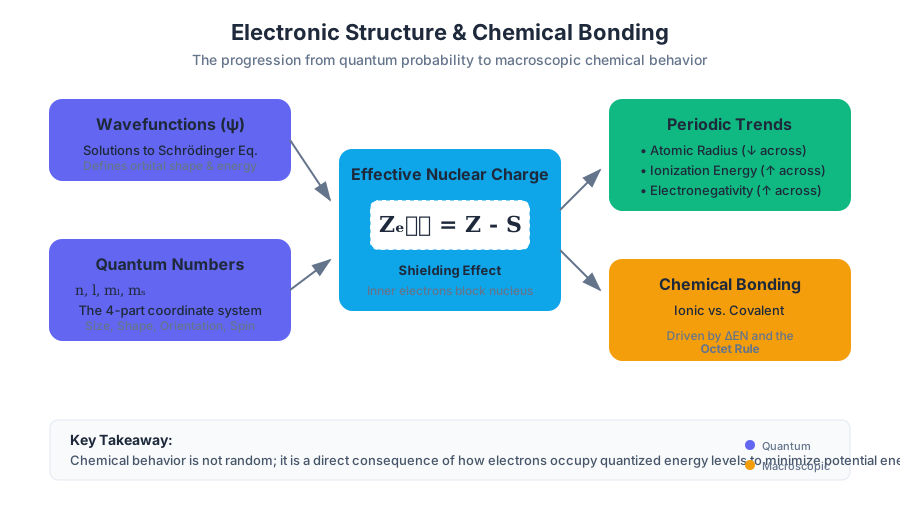
The transition from the Bohr model—which depicted electrons in neat, planetary orbits—to the Quantum Mechanical Model represents one of the most significant shifts in scientific history. Instead of deterministic paths, we use wavefunctions ($\psi$) to describe the probability of finding an electron in a specific region of space.

Wave-Particle Duality and the Schrödinger Equation

At the heart of electronic structure is the Schrödinger Equation. It treats the electron not as a point mass, but as a standing wave. The solutions to this equation, known as wavefunctions, provide the energy levels and the shapes of the orbitals.

The Heisenberg Uncertainty Principle: It is fundamentally impossible to determine simultaneously both the exact position and the exact momentum of an electron. This necessitates the use of "probability clouds" rather than trajectories.

Quantum Numbers

To uniquely identify an electron's state within an atom, we use four quantum numbers. These act as a "coordinate system" for the electron's energy and location.

Quantum Number	Symbol	Allowed Values	Physical Significance
Principal	$n$	$1, 2, 3, \dots$	Shell level, primary energy, and size.
Angular Momentum	$l$	$0$ to $n-1$	Shape of the orbital (s, p, d, f).
Magnetic	$m_l$	$-l$ to $+l$	Orientation of the orbital in 3D space.
Spin	$m_s$	$+1/2, -1/2$	Direction of the electron's intrinsic spin.

Implementation: Calculating Radial Probability

In computational chemistry, we often need to visualize these probability densities. The following Python snippet demonstrates how to calculate the radial probability distribution for a hydrogenic 1s orbital.

import numpy as np
import matplotlib.pyplot as plt

def radial_wavefunction_1s(r, Z=1):
    """
    Calculates the value of the 1s radial wavefunction for a hydrogen-like atom.
    psi = (1/sqrt(pi)) * (Z/a0)**(3/2) * exp(-Z*r/a0)
    """
    a0 = 1.0  # Bohr radius in atomic units
    prefactor = (1.0 / np.sqrt(np.pi)) * (Z / a0)**(1.5)
    return prefactor * np.exp(-Z * r / a0)

def radial_probability_density(r, Z=1):
    """
    P(r) = 4 * pi * r^2 * |psi|^2
    """
    psi = radial_wavefunction_1s(r, Z)
    return 4 * np.pi * (r**2) * (psi**2)

# Simulation parameters
r_values = np.linspace(0, 5, 500)
prob_density = radial_probability_density(r_values)

# Find the most probable radius (should be a0 for Z=1)
max_r = r_values[np.argmax(prob_density)]
print(f"Most probable radius: {max_r:.4f} Bohr radii")

Periodic Trends: The Macro-Scale Manifestation

The periodic table is not merely a list of elements; it is a map of electronic structure. As we populate orbitals according to the Aufbau Principle, Hund's Rule, and the Pauli Exclusion Principle, specific patterns emerge in atomic properties.

Effective Nuclear Charge ($Z_{eff}$)

The most critical concept in understanding trends is shielding. Inner-shell electrons "shield" outer electrons from the full positive charge of the nucleus. The net charge experienced by a valence electron is the Effective Nuclear Charge.

Z_{eff} = Z - S

Where $Z$ is the atomic number and $S$ is the shielding constant (often estimated using Slater's Rules).

Primary Trends Summary

The interplay between $Z_{eff}$ and the principal quantum number $n$ dictates the following trends:

Property	Across a Period (Left to Right)	Down a Group (Top to Bottom)	Reason
Atomic Radius	Decreases	Increases	Increasing $Z_{eff}$ pulls electrons closer; increasing $n$ adds shells.
Ionization Energy	Increases	Decreases	Stronger nuclear attraction makes electron removal harder.
Electronegativity	Increases	Decreases	Atoms have a stronger "pull" on shared electrons as $Z_{eff}$ rises.
Electron Affinity	Becomes more negative	Becomes less negative	Atoms release more energy when gaining an electron to fill a shell.

Common Pitfall: The "Half-Filled Shell" Exception

Students often expect Ionization Energy (IE) to increase perfectly linearly across a period. However, Nitrogen ($2p^3$) has a higher first IE than Oxygen ($2p^4$). This is because Nitrogen has a stable, half-filled p-subshell. Removing an electron from Oxygen relieves the electron-electron repulsion of the first paired p-orbital, making it energetically "easier" than expected.

Chemical Bonding: The Quest for Stability

Atoms bond to reach a state of minimum potential energy. This is usually achieved by attaining a stable electronic configuration, often resembling a noble gas (the Octet Rule).

Ionic vs. Covalent Bonding

Bonding exists on a continuum. The determining factor is the difference in electronegativity ($\Delta EN$) between the two atoms.

1. Ionic Bonding ($\Delta EN > 1.8$): A complete transfer of electrons. The bond is held together by electrostatic (Coulombic) forces.
2. Covalent Bonding ($\Delta EN < 1.8$): Electrons are shared.
   • Polar Covalent: Unequal sharing (e.g., $H-Cl$).
   • Non-polar Covalent: Equal sharing (e.g., $O=O$).

Formal Charge: The Bookkeeping of Electrons

When multiple Lewis structures are possible, we use Formal Charge (FC) to determine the most plausible one. The goal is to have formal charges as close to zero as possible.

Theorem: The sum of all formal charges in a molecule must equal the overall charge of the molecule.

FC = V - N - \frac{B}{2}

Where $V$ = valence electrons, $N$ = non-bonding electrons (lone pairs), and $B$ = bonding electrons.

Example: The Nitrate Ion ($NO_3^-$)

Nitrate exhibits resonance. No single Lewis structure accurately describes the molecule. Instead, the actual structure is an average of three resonance contributors, where the bond order is $1.33$ rather than a discrete single or double bond.

# Using Open Babel to check the formal charge and bond orders of a SMILES string
# Input: Nitrate ion [O-][N+](=O)[O-]
obabel -:"[O-][N+](=O)[O-]" -oreport

VSEPR Theory: Predicting Molecular Geometry

Valence Shell Electron Pair Repulsion (VSEPR) theory posits that electron groups (bonds and lone pairs) around a central atom will arrange themselves as far apart as possible to minimize electrostatic repulsion.

Steric Number and Geometry

The Steric Number (SN) is the sum of the number of atoms bonded to the central atom and the number of lone pairs on that atom.

SN	Electron Geometry	Lone Pairs	Molecular Geometry	Bond Angle
2	Linear	0	Linear	180°
3	Trigonal Planar	0	Trigonal Planar	120°
3	Trigonal Planar	1	Bent	< 120°
4	Tetrahedral	0	Tetrahedral	109.5°
4	Tetrahedral	1	Trigonal Pyramidal	107°
4	Tetrahedral	2	Bent	104.5°
5	Trigonal Bipyramidal	0	Trigonal Bipyramidal	90°, 120°
6	Octahedral	0	Octahedral	90°

The Impact of Lone Pairs

Lone pairs occupy more space than bonding pairs. This is because a lone pair is attracted to only one nucleus, allowing its electron cloud to spread out. This "expansion" pushes the adjacent bonding pairs closer together, resulting in compressed bond angles. For example, while methane ($CH_4$) has $109.5^\circ$ angles, water ($H_2O$) with two lone pairs has a compressed angle of $104.5^\circ$.

Advanced Perspective: Beyond the Octet

While the Octet Rule is a powerful heuristic, it fails for several classes of molecules:

1. Electron-Deficient Molecules: Elements like Beryllium and Boron often form stable compounds with fewer than 8 electrons (e.g., $BF_3$).
2. Odd-Electron Molecules: Radicals like $NO$ have an unpaired electron and cannot satisfy the octet.
3. Hypervalent Molecules: Elements in Period 3 and below (e.g., $P, S, I$) can expand their octet by utilizing d-orbitals (e.g., $SF_6$, $PCl_5$).

Data Representation: Chemical Properties Database

In a professional setting, chemical data is stored in structured formats to facilitate high-throughput screening or ML model training.

-- Schema for storing molecular properties derived from electronic structure
CREATE TABLE molecules (
    molecule_id SERIAL PRIMARY KEY,
    smiles_string TEXT UNIQUE NOT NULL,
    molecular_weight DECIMAL,
    dipole_moment DECIMAL, -- Derived from VSEPR and electronegativity
    homo_energy DECIMAL,    -- Highest Occupied Molecular Orbital
    lumo_energy DECIMAL,    -- Lowest Unoccupied Molecular Orbital
    point_group VARCHAR(10) -- Symmetry classification
);

INSERT INTO molecules (smiles_string, molecular_weight, dipole_moment, point_group)
VALUES ('O', 18.015, 1.85, 'C2v'),
       ('CO2', 44.01, 0.00, 'Dinfh');

Summary of Theoretical Frameworks

To master chemical bonding, one must navigate between different levels of abstraction. While VSEPR is excellent for geometry, it does not explain why bonds form energetically. For that, we look to Valence Bond Theory (hybridization) and Molecular Orbital (MO) Theory.

• Valence Bond Theory: Describes bonds as the overlap of atomic orbitals (e.g., $sp^3$ hybridization in Carbon).
• Molecular Orbital Theory: Describes electrons as belonging to the entire molecule, creating bonding and anti-bonding orbitals. This theory correctly predicts the paramagnetism of Oxygen ($O_2$), which Lewis structures fail to do.

Key Terms for Review

• Orbital: A mathematical function describing the location and wave-like behavior of an electron.
• Isoelectronic: Atoms or ions that have the same electron configuration (e.g., $Na^+$ and $Ne$).
• Paramagnetism: A property of materials with unpaired electrons that are attracted to magnetic fields.
• Dipole Moment: A measure of the separation of positive and negative electrical charges within a system.
• Hybridization: The mixing of atomic orbitals to form new hybrid orbitals suitable for the pairing of electrons to form chemical bonds.

Final Insight

Electronic structure is the "source code" of the universe. Every biological process, every material property of a new alloy, and every pharmaceutical interaction is a direct consequence of the way electrons choose to occupy space and minimize their energy. By mastering these quantum rules, we gain the ability to engineer the world at its most fundamental level.

States of Matter and Thermochemistry

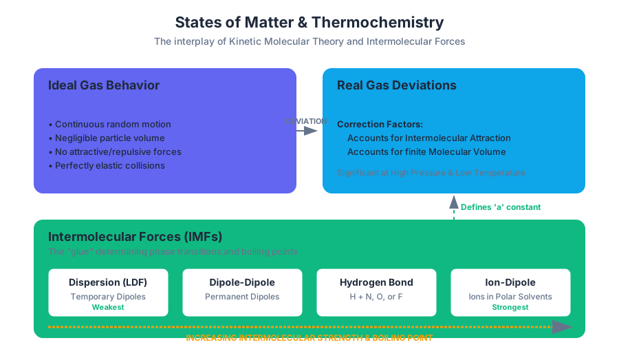
The study of matter is fundamentally a study of energy and interaction. While introductory chemistry often treats substances as static entities, a deep-dive into the States of Matter and Thermochemistry reveals a dynamic landscape where microscopic forces and macroscopic energy transfers dictate the behavior of everything from the air in a combustion engine to the folding of proteins in a cell. This section bridges the gap between the Kinetic Molecular Theory of gases and the thermodynamic laws that govern heat flow and phase transitions.

The Gaseous State and the Ideal Gas Law

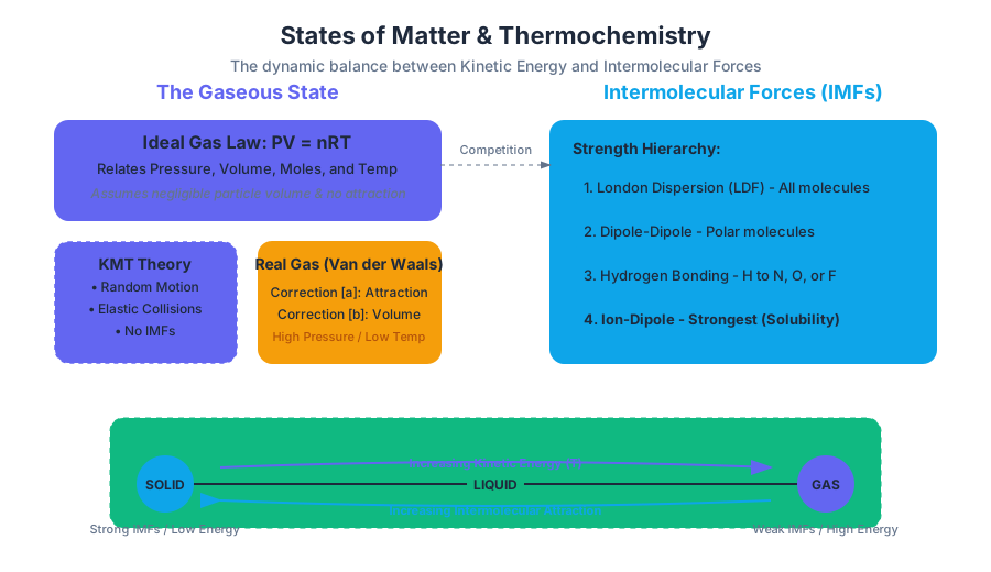
Gases represent the most chaotic state of matter, where kinetic energy significantly outweighs the attractive forces between particles. To model this behavior, we use the Ideal Gas Law, a cornerstone of classical thermodynamics that relates the physical properties of a gas sample.

What it is

The Ideal Gas Law is an equation of state defined as:

PV = nRT Where P is absolute pressure, V is volume, n is the number of moles, R is the universal gas constant (8.314 J/mol·K or 0.08206 L·atm/mol·K), and T is the absolute temperature in Kelvin.

How it Works: Kinetic Molecular Theory (KMT)

The validity of the Ideal Gas Law rests on the Kinetic Molecular Theory, which posits four primary assumptions:

1. Gas particles are in continuous, random motion.
2. The volume of the particles themselves is negligible compared to the container volume.
3. Particles exert no attractive or repulsive forces on each other.
4. Collisions are perfectly elastic (no net loss of kinetic energy).

Real Gas Deviations

In reality, no gas is truly "ideal." At high pressures, the volume of the molecules becomes significant. At low temperatures, Intermolecular Forces (IMFs) cause particles to "stick" together, reducing the pressure exerted on container walls. To account for this, engineers use the Van der Waals Equation:

[P + a(n/V)²][V - nb] = nRT Here, a accounts for attractive forces and b accounts for the finite volume of the gas molecules.

Law Name	Constant Variables	Relationship	Mathematical Form
Boyle’s Law	n, T	Pressure is inversely proportional to Volume	P1V1 = P2V2
Charles’s Law	n, P	Volume is directly proportional to Temperature	V1/T1 = V2/T2
Avogadro’s Law	P, T	Volume is directly proportional to Moles	V1/n1 = V2/n2
Gay-Lussac’s Law	n, V	Pressure is directly proportional to Temperature	P1/T1 = P2/T2

Implementation: Calculating Real Gas Behavior

The following Python implementation demonstrates how to calculate the pressure of a real gas using the Van der Waals equation compared to the Ideal Gas Law.

import numpy as np

def calculate_gas_pressures(n, V, T, a, b):
    """
    Compares Ideal Gas Law vs Van der Waals Equation.
    n: moles (mol)
    V: volume (L)
    T: temperature (K)
    a: attraction constant (L^2*atm/mol^2)
    b: volume constant (L/mol)
    """
    R = 0.08206  # L*atm/(mol*K)
    
    # Ideal Gas Law: P = nRT / V
    p_ideal = (n * R * T) / V
    
    # Van der Waals: P = (nRT / (V - nb)) - a(n/V)^2
    p_real = ((n * R * T) / (V - n * b)) - a * (n / V)**2
    
    deviation = abs(p_ideal - p_real) / p_real * 100
    
    return {
        "Ideal Pressure (atm)": round(p_ideal, 4),
        "Real Pressure (atm)": round(p_real, 4),
        "Percent Deviation (%)": round(deviation, 2)
    }

# Example: Chlorine gas (Cl2) at high pressure
# a = 6.49, b = 0.0562 for Cl2
results = calculate_gas_pressures(n=10.0, V=2.0, T=300, a=6.49, b=0.0562)
print(results)

Intermolecular Forces (IMFs)

While gases are defined by the absence of interaction, liquids and solids are defined by them. Intermolecular Forces are the non-covalent attractive forces that hold molecules together. They are the "glue" of the physical world.

The Hierarchy of Forces

IMFs vary in strength based on molecular polarity and electron cloud polarizability.

1. London Dispersion Forces (LDF): Present in all molecules. Caused by temporary fluctuations in electron density creating "instantaneous dipoles." Strength increases with molar mass (polarizability).
2. Dipole-Dipole Interactions: Occur between polar molecules with permanent dipoles.
3. Hydrogen Bonding: A specific, ultra-strong dipole-dipole interaction occurring when H is bonded to N, O, or F.
4. Ion-Dipole Forces: The strongest IMF, occurring between an ion and a polar molecule (critical for solubility in water).

Force Type	Relative Strength	Requirement	Example
Dispersion	Weakest	All molecules	CH4, He, I2
Dipole-Dipole	Moderate	Permanent Dipole	HCl, CH3Cl
Hydrogen Bond	Strong	H-F, H-O, or H-N	H2O, NH3, DNA base pairs
Ion-Dipole	Strongest	Ion + Polar solvent	NaCl in H2O

Why IMFs Matter: Phase Transitions

The boiling point and melting point of a substance are direct proxies for the strength of its IMFs. To transition from liquid to gas, a molecule must gain enough kinetic energy to overcome the "stickiness" of its neighbors.

The Vapor Pressure Paradox: As IMFs increase, vapor pressure decreases. This is because fewer molecules have the energy required to escape the liquid phase into the gas phase at a given temperature.

Mathematical Derivation: The Lennard-Jones Potential

In computational chemistry, the interaction between two non-bonded atoms is often modeled using the Lennard-Jones 6-12 Potential, which describes the balance between attractive dispersion forces and Pauli repulsion.

V_{LJ}(r) = 4\epsilon \left[ \left( \frac{\sigma}{r} \right)^{12} - \left( \frac{\sigma}{r} \right)^{6} \right]

• r: Distance between particles.
• ε: Depth of the potential well (strength of attraction).
• σ: Distance at which the potential is zero (particle size).
• The r^-12 term represents short-range repulsion (Pauli exclusion).
• The r^-6 term represents long-range attraction (Van der Waals/Dispersion).

Thermochemistry and Enthalpy

Thermochemistry is the study of heat absorbed or released during chemical reactions and physical changes. It is a subset of thermodynamics, focusing specifically on the First Law of Thermodynamics: Energy cannot be created or destroyed, only transformed.

Enthalpy (ΔH)

In most laboratory settings, reactions occur at constant pressure. Under these conditions, the heat flow (q) is equal to the change in Enthalpy (ΔH).

Enthalpy (H): A state function defined as H = U + PV. The change in enthalpy (ΔH) represents the heat exchanged by the system at constant pressure.

• Exothermic (ΔH < 0): The system releases heat to the surroundings (e.g., combustion).
• Endothermic (ΔH > 0): The system absorbs heat from the surroundings (e.g., photosynthesis, ice melting).

Standard Enthalpy of Formation (ΔH°f)

To standardize measurements, we use the Standard Enthalpy of Formation, which is the change in enthalpy when 1 mole of a substance is formed from its pure elements in their most stable form at 1 atm and 25°C.

Hess’s Law

Since enthalpy is a state function (independent of the path taken), we can calculate the ΔH of a complex reaction by summing the ΔH values of its individual steps.

\Delta H_{reaction} = \sum n\Delta H_f^\circ(\text{products}) - \sum m\Delta H_f^\circ(\text{reactants})

Real-World Usage: Simulation Configuration

In professional molecular dynamics or thermochemical modeling (like using the NASA Polynomials for combustion), enthalpy is defined in configuration files to predict flame temperature and energy output.

# Simulation Parameters for Methane Combustion
reaction_id: CH4_O2_Combustion
thermo_model: Shomate_Equation
species:
  CH4:
    hf_298: -74.8  # kJ/mol
    cp_coeffs: [25.9, 0.07, -0.00001] # Temperature dependent heat capacity
  O2:
    hf_298: 0.0    # Elemental state
    cp_coeffs: [29.1, 0.01, -0.000001]
  CO2:
    hf_298: -393.5
  H2O_g:
    hf_298: -241.8

conditions:
  pressure_atm: 1.0
  initial_temp_K: 298.15
  equivalence_ratio: 1.0

Calorimetry: Measuring the Heat of Reaction

Calorimetry is the experimental backbone of thermochemistry. It involves measuring the temperature change of a known mass of substance (usually water) to determine the heat exchanged by a process.

Specific Heat Capacity (c)

The amount of heat required to raise the temperature of 1 gram of a substance by 1 degree Celsius.

q = m * c * ΔT Where q is heat (Joules), m is mass (g), c is specific heat (J/g·°C), and ΔT is the change in temperature.

Types of Calorimeters

1. Constant-Pressure Calorimetry (Coffee-Cup): Used for reactions in solution. Since the pressure is constant (atmospheric), q_soln = ΔH.
2. Constant-Volume Calorimetry (Bomb): Used for combustion reactions. The rigid "bomb" prevents volume change, meaning no PΔV work is done. Here, the measured heat q_v equals the change in internal energy (ΔU), not enthalpy.

Feature	Coffee-Cup Calorimeter	Bomb Calorimeter
Constant Parameter	Pressure (P)	Volume (V)
Measured Heat	Enthalpy (ΔH)	Internal Energy (ΔU)
Typical Use Case	Acid-Base Neutralization	Fuel Combustion
Complexity	Low (Styrofoam cup)	High (Steel pressure vessel)

Common Pitfalls in Calorimetry Calculations

• Sign Conventions: Remember that q_system = -q_surroundings. If the water (surroundings) gets hotter, the reaction (system) is exothermic (negative ΔH).
• Heat Capacity of the Calorimeter: In high-precision work, the calorimeter itself absorbs heat. This is accounted for using the "Calorimeter Constant" (C_cal).
  • q_total = (m_water * c_water * ΔT) + (C_cal * ΔT)
• State of Matter: The enthalpy of formation for H2O(l) is different from H2O(g). Always check the phase in your thermochemical equations.

Worked Example: Hess's Law Calculation

Calculate the ΔH for the reaction: C(graphite) + 2H2(g) → CH4(g) Given:

1. C(graphite) + O2(g) → CO2(g) (ΔH = -393.5 kJ)
2. H2(g) + 1/2 O2(g) → H2O(l) (ΔH = -285.8 kJ)
3. CH4(g) + 2O2(g) → CO2(g) + 2H2O(l) (ΔH = -890.3 kJ)

Step 1: Keep Eq 1 as is (provides 1C). Step 2: Multiply Eq 2 by 2 (provides 2H2). ΔH = 2 * (-285.8) = -571.6 kJ. Step 3: Reverse Eq 3 (puts CH4 on the product side). ΔH = +890.3 kJ. Sum: -393.5 + (-571.6) + 890.3 = -74.8 kJ/mol.

Summary of State Transitions

The interplay between kinetic energy (temperature) and IMFs determines the phase of matter.

Transition	Name	Energy Change	IMF Effect
Solid → Liquid	Melting/Fusion	Endothermic	Overcoming rigid lattice
Liquid → Gas	Vaporization	Endothermic	Breaking all IMFs
Gas → Liquid	Condensation	Exothermic	Re-establishing IMFs
Liquid → Solid	Freezing	Exothermic	Forming rigid lattice
Solid → Gas	Sublimation	Endothermic	Direct bypass of liquid

Chemical Kinetics and Equilibrium

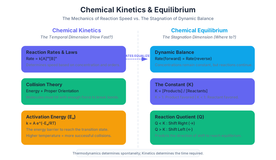
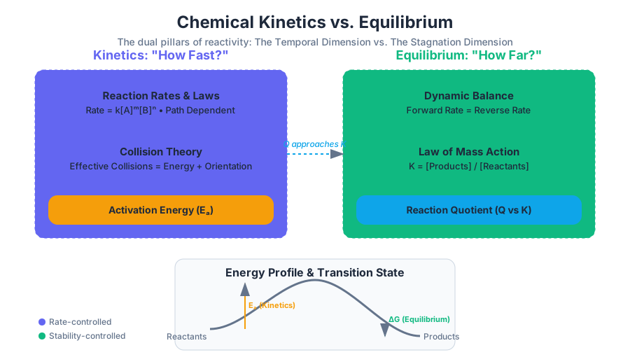
Chemical kinetics and equilibrium represent the two fundamental pillars of chemical reactivity: the temporal dimension (how fast a reaction occurs) and the stagnation dimension (where a reaction eventually settles). While thermodynamics tells us whether a reaction is spontaneous, it remains silent on the time required to reach the finish line. A diamond is thermodynamically unstable relative to graphite, yet the kinetics of that transition are so slow that the process is effectively non-existent on human timescales. This article explores the mechanics of reaction rates, the energy barriers of molecular collisions, and the delicate balance of reversible systems.

Chemical Kinetics: The Mechanics of Speed

Chemical Kinetics is the study of reaction rates and the molecular pathways (mechanisms) by which reactants transform into products. Understanding kinetics is not merely academic; it is the difference between an industrial process that takes hours and one that takes seconds, or a medication that releases its active ingredient over twelve hours versus one that peaks in minutes.

Reaction Rates and Rate Laws

The reaction rate is defined as the change in concentration of a reactant or product per unit of time. For a general reaction $aA + bB \rightarrow cC + dD$, the rate is expressed as:

$$Rate = -\frac{1}{a}\frac{\Delta[A]}{\Delta t} = \frac{1}{c}\frac{\Delta[C]}{\Delta t}$$

However, the rate is rarely constant. It typically depends on the concentrations of the reactants, a relationship defined by the Differential Rate Law:

$$Rate = k[A]^m[B]^n$$

Where:

• $k$ is the rate constant, a temperature-dependent proportionality constant.
• $m$ and $n$ are the reaction orders, determined experimentally and not necessarily equal to the stoichiometric coefficients.

Integrated Rate Laws

To predict the concentration of a substance at a specific time, we use Integrated Rate Laws. These equations vary based on the overall order of the reaction.

Reaction Order	Rate Law	Integrated Rate Law	Units of $k$	Half-life ($t_{1/2}$)
Zero	$Rate = k$	$[A]_t = -kt + [A]_0$	$M \cdot s^{-1}$	$[A]_0 / 2k$
First	$Rate = k[A]$	$\ln[A]_t = -kt + \ln[A]_0$	$s^{-1}$	$0.693 / k$
Second	$Rate = k[A]^2$	$1/[A]_t = kt + 1/[A]_0$	$M^{-1} \cdot s^{-1}$	$1 / (k[A]_0)$

Collision Theory and Activation Energy

For a reaction to occur, molecules must collide. However, collision alone is insufficient. According to Collision Theory, two criteria must be met:

1. Sufficient Energy: The collision must possess enough kinetic energy to overcome the Activation Energy ($E_a$), the minimum energy required to break existing bonds and form the transition state (or activated complex).
2. Correct Orientation: The molecules must hit each other in a geometry that allows new bonds to form.

The relationship between temperature, activation energy, and the rate constant is quantified by the Arrhenius Equation:

$$k = A e^{-E_a / RT}$$

Where $A$ is the frequency factor (representing collision frequency and orientation probability), $R$ is the ideal gas constant, and $T$ is the absolute temperature.

Implementation: Numerical Integration of Reaction Rates

In complex systems with multiple competing reactions, analytical solutions for concentration are often impossible. We employ numerical methods like the 4th-order Runge-Kutta (RK4) to simulate the concentration profile over time.

import numpy as np
import matplotlib.pyplot as plt

def reaction_system(t, y, k_forward, k_backward):
    """
    Defines the ODEs for a reversible first-order reaction: A <-> B
    d[A]/dt = -k_f[A] + k_b[B]
    d[B]/dt =  k_f[A] - k_b[B]
    """
    A, B = y
    dA_dt = -k_forward * A + k_backward * B
    dB_dt = k_forward * A - k_backward * B
    return np.array([dA_dt, dB_dt])

def rk4_step(f, t, y, dt, *args):
    k1 = f(t, y, *args)
    k2 = f(t + dt/2, y + dt/2 * k1, *args)
    k3 = f(t + dt/2, y + dt/2 * k2, *args)
    k4 = f(t + dt, y + dt * k3, *args)
    return y + (dt/6) * (k1 + 2*k2 + 2*k3 + k4)

# Parameters
k_f, k_b = 0.5, 0.2
y0 = np.array([1.0, 0.0]) # Initial concentrations [A]=1.0, [B]=0.0
t, dt, steps = 0, 0.1, 100
results = []

for _ in range(steps):
    results.append((t, y0[0], y0[1]))
    y0 = rk4_step(reaction_system, t, y0, dt, k_f, k_b)
    t += dt

# Results show [A] decaying and [B] rising until equilibrium is reached.

Chemical Equilibrium: The Dynamic Balance

When a reaction occurs in a closed system, it eventually reaches a state where the concentrations of reactants and products no longer change. This is Chemical Equilibrium. It is important to realize that equilibrium is dynamic, not static; the forward and reverse reactions continue to occur, but at exactly the same rate.

The Equilibrium Constant ($K$)

The Law of Mass Action states that for a reversible reaction at equilibrium, the ratio of product concentrations to reactant concentrations (each raised to the power of their coefficients) is constant at a given temperature.

$$K_c = \frac{[C]^c[D]^d}{[A]^a[B]^b}$$

The Equilibrium Principle: The value of $K$ indicates the extent of a reaction. A large $K$ ($> 10^3$) implies the reaction goes nearly to completion, while a small $K$ ($< 10^{-3}$) implies the reaction hardly proceeds at all.

Reaction Quotient ($Q$) vs. Equilibrium Constant ($K$)

To determine if a system is at equilibrium or which direction it must shift to reach it, we calculate the Reaction Quotient ($Q$) using current (non-equilibrium) concentrations.

Condition	Meaning	Direction of Shift
$Q < K$	Too much reactant, not enough product	Shift Right (towards products)
$Q > K$	Too much product, not enough reactant	Shift Left (towards reactants)
$Q = K$	System is at chemical equilibrium	No net change

Mathematical Derivation: $K_p$ vs $K_c$

For gaseous reactions, equilibrium can be expressed in terms of partial pressures ($K_p$). The relationship between $K_p$ and $K_c$ is derived from the Ideal Gas Law ($PV = nRT$).

\begin{aligned}
P_i &= \frac{n_i}{V}RT = [M]_i RT \\
K_p &= \frac{(P_C)^c (P_D)^d}{(P_A)^a (P_B)^b} \\
K_p &= \frac{([C]RT)^c ([D]RT)^d}{([A]RT)^a ([B]RT)^b} \\
K_p &= \frac{[C]^c [D]^d}{[A]^a [B]^b} (RT)^{(c+d)-(a+b)} \\
K_p &= K_c (RT)^{\Delta n}
\end{aligned}

Where $\Delta n$ is the change in moles of gas (moles of gaseous products - moles of gaseous reactants).

Le Chatelier’s Principle: Responding to Stress

If a system at equilibrium is subjected to a change in concentration, pressure, or temperature, the system will shift its equilibrium position to counteract the effect of the disturbance.

Stressors and Responses

1. Concentration: Adding a reactant shifts the equilibrium toward the products. Removing a product does the same (a common tactic in industrial synthesis).
2. Pressure/Volume: For reactions involving gases, decreasing the volume (increasing pressure) shifts the equilibrium toward the side with fewer moles of gas.
3. Temperature: This is the only stressor that actually changes the value of $K$.
   • In an Exothermic reaction (heat is a product), increasing temperature shifts the equilibrium toward reactants ($K$ decreases).
   • In an Endothermic reaction (heat is a reactant), increasing temperature shifts the equilibrium toward products ($K$ increases).

Disturbance	Shift Direction (Exothermic)	Shift Direction (Endothermic)	Change in $K$
Increase Temp	Left	Right	Yes
Decrease Temp	Right	Left	Yes
Increase Pressure	Toward fewer gas moles	Toward fewer gas moles	No
Add Catalyst	No shift	No shift	No

Acid-Base Equilibria: A Specialized Framework

One of the most critical applications of equilibrium is in the behavior of acids and bases in aqueous solutions. This is governed by the transfer of protons ($H^+$).

The Brønsted-Lowry Theory

An acid is a proton donor, and a base is a proton acceptor. Every acid has a conjugate base, and every base has a conjugate acid.

HA(aq) + H_2O(l) \rightleftharpoons H_3O^+(aq) + A^-(aq)

The Autoionization of Water

Even pure water exists in equilibrium with its ions:

H_2O(l) + H_2O(l) \rightleftharpoons H_3O^+(aq) + OH^-(aq)

The equilibrium constant for this process is $K_w = [H_3O^+][OH^-] = 1.0 \times 10^{-14}$ at 25°C. This constant forms the basis of the pH scale: $$pH = -\log[H_3O^+]$$

Weak Acids and Bases

Unlike strong acids which dissociate completely, weak acids reach an equilibrium defined by the acid dissociation constant ($K_a$): $$K_a = \frac{[H_3O^+][A^-]}{[HA]}$$ The smaller the $K_a$, the weaker the acid. A similar constant, $K_b$, exists for weak bases.

Buffers and the Henderson-Hasselbalch Equation

A buffer is a solution that resists changes in pH when small amounts of acid or base are added. It consists of a weak acid and its conjugate base. The pH of a buffer is calculated using the Henderson-Hasselbalch Equation:

$$pH = pK_a + \log\left(\frac{[Base]}{[Acid]}\right)$$

Real-World Usage: Simulation and Calculation

In laboratory or industrial settings, calculating the exact pH of a complex buffer or the result of a titration requires solving the charge balance and mass balance equations.

# Example: Using a hypothetical CLI tool 'chem-calc' to determine 
# the pH of a 0.1M Acetic Acid / 0.1M Sodium Acetate buffer.

$ chem-calc equilibrium --acid "CH3COOH" --ka 1.8e-5 --conc_acid 0.1 --conc_base 0.1

> Result:
> [H3O+] = 1.80e-05 M
> pH = 4.74
> Dissociation: 0.018%
> Status: Buffer system stable.

Common Pitfalls and Misconceptions

• Confusing Rate with Equilibrium: A reaction can have a very large $K$ (highly favorable) but a very small $k$ (extremely slow). Do not assume that because a reaction is "spontaneous," it will happen quickly.
• The Role of Catalysts: A catalyst increases the rate of reaction by providing an alternative pathway with a lower activation energy. It does not change the equilibrium constant or the position of equilibrium. It simply helps the system reach equilibrium faster.
• Pure Solids and Liquids: In the equilibrium expression, the activities of pure solids and pure liquids are defined as 1. Therefore, they do not appear in the $K_c$ or $K_p$ expressions. Adding more of a solid reactant will not shift the equilibrium position.
• Temperature and $K$: Many students forget that $K$ is constant only if temperature is constant. If a problem involves a temperature change, you must find the new $K$ (often using the Van 't Hoff equation).

Summary of Key Parameters

Parameter	Symbol	Definition	Influence
Rate Constant	$k$	Speed of elementary step	Temperature, $E_a$, Catalyst
Activation Energy	$E_a$	Energy barrier to react	Molecular structure, Catalyst
Equilibrium Constant	$K$	Ratio of products/reactants	Temperature, $\Delta G^\circ$
Reaction Quotient	$Q$	Current state of system	Instantaneous concentrations
Acid Dissociation	$K_a$	Strength of weak acid	Molecular structure, Solvent

Thermodynamics and Electrochemistry

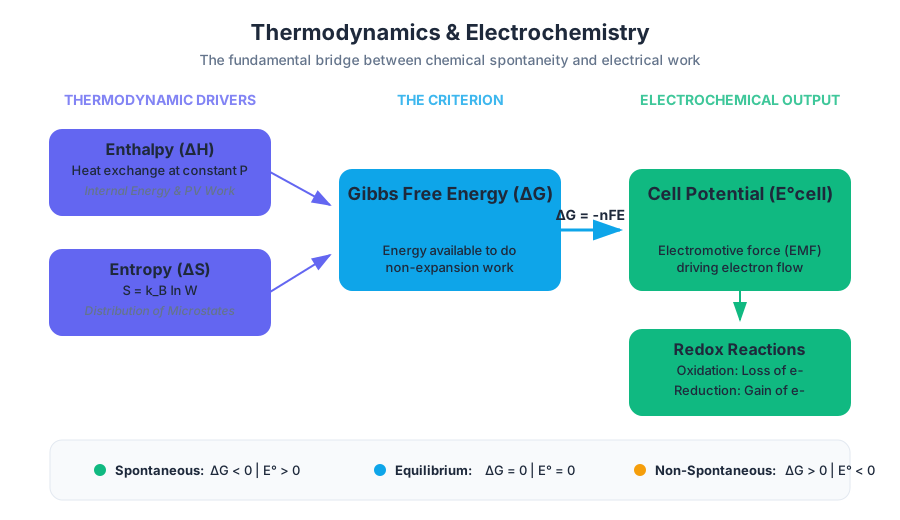
The study of chemical change is governed by two fundamental questions: "Can it happen?" and "How much energy can we extract if it does?" While kinetics describes the rate of a reaction, Thermodynamics provides the ultimate roadmap for spontaneity and equilibrium. When these thermodynamic principles are applied to the movement of electrons, we enter the domain of Electrochemistry—the bridge between chemical bonding and electrical work.

This article explores the rigorous framework connecting entropy, free energy, and the electrochemical potential, providing the technical foundation required to understand everything from cellular respiration to the next generation of solid-state batteries.

Entropy and the Second Law

At the heart of all spontaneous processes lies Entropy ($S$), a state function that quantifies the distribution of energy within a system. Unlike energy, which is conserved, entropy is cumulative.

The Second Law of Thermodynamics: In any spontaneous process, the total entropy of the universe ($S_{universe} = S_{system} + S_{surroundings}$) must increase.

Microstates and Statistical Mechanics

From a statistical perspective, entropy is defined by the Boltzmann Equation: $$S = k_B \ln W$$ where $k_B$ is the Boltzmann constant ($1.38 \times 10^{-23} J/K$) and $W$ is the number of microstates—the specific microscopic configurations (position and momentum of particles) that correspond to a particular macroscopic state.

Factors Influencing Entropy

Entropy is not merely "disorder"; it is a measure of energy dispersal. Several factors predictably increase the number of available microstates:

1. Phase Changes: Transitioning from solid to liquid to gas significantly increases positional entropy.
2. Temperature: Higher kinetic energy allows particles to access more vibrational and rotational energy levels.
3. Molecular Complexity: Larger molecules have more internal degrees of freedom (bonds that can vibrate or rotate).
4. Dissolution: Mixing solutes into solvents generally increases the volume available to each particle.

State Change	Entropy Trend ($\Delta S$)	Physical Justification
$S \rightarrow L \rightarrow G$	Positive (+)	Massive increase in translational microstates.
$N_2(g) + 3H_2(g) \rightarrow 2NH_3(g)$	Negative (-)	Reduction in the total moles of gas particles.
Dissolving $NaCl(s)$ in $H_2O$	Positive (+)	Lattice breakdown increases ion mobility.
Heating $Cu(s)$ from 298K to 500K	Positive (+)	Increased population of higher energy vibrational states.

Gibbs Free Energy ($G$): The Criterion for Spontaneity

While the Second Law focuses on the universe, chemists require a metric focused solely on the system. This is provided by the Gibbs Free Energy ($G$), defined as the energy available to do "useful" (non-expansion) work at constant temperature and pressure.

The Gibbs-Helmholtz Equation

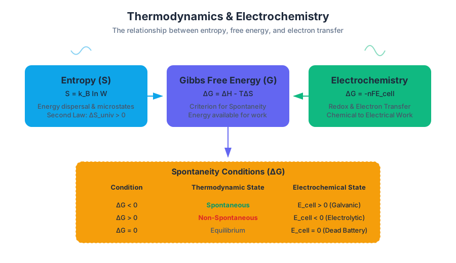
The relationship between enthalpy ($H$), entropy ($S$), and temperature ($T$) is expressed as: $$\Delta G = \Delta H - T\Delta S$$

This equation acts as a balance between the drive toward minimum energy (enthalpy) and maximum dispersal (entropy).

Spontaneity Conditions

The sign of $\Delta G$ determines the direction of chemical change:

• $\Delta G < 0$: Spontaneous (Exergonic)
• $\Delta G > 0$: Non-spontaneous (Endergonic)
• $\Delta G = 0$: Equilibrium

$\Delta H$	$\Delta S$	Spontaneity Condition	Example
Negative (-)	Positive (+)	Spontaneous at all temperatures	$2O_3(g) \rightarrow 3O_2(g)$
Positive (+)	Negative (-)	Non-spontaneous at all temperatures	$3O_2(g) \rightarrow 2O_3(g)$
Negative (-)	Negative (-)	Spontaneous at LOW temperatures	Freezing of water
Positive (+)	Positive (+)	Spontaneous at HIGH temperatures	Vaporization of water

Low-Level Implementation: Spontaneity Calculator

The following Python snippet demonstrates how a computational chemist might evaluate the spontaneity of a reaction across a temperature gradient using the NumPy library for vectorized operations.

import numpy as np

def calculate_spontaneity(delta_h, delta_s, temp_range):
    """
    Calculates Gibbs Free Energy over a range of temperatures.
    delta_h: Enthalpy in kJ/mol
    delta_s: Entropy in J/(mol*K)
    temp_range: tuple (start_t, end_t, step) in Kelvin
    """
    # Convert Delta H to Joules for unit consistency
    h_j = delta_h * 1000
    
    temps = np.arange(temp_range[0], temp_range[1], temp_range[2])
    # Delta G = Delta H - T * Delta S
    gibbs_values = h_j - (temps * delta_s)
    
    results = []
    for t, g in zip(temps, gibbs_values):
        status = "Spontaneous" if g < 0 else "Non-Spontaneous"
        results.append({"Temp": t, "Gibbs": g/1000, "Status": status})
        
    return results

# Example: Haber Process N2 + 3H2 -> 2NH3
# Delta H = -92.22 kJ/mol, Delta S = -198.75 J/(mol*K)
analysis = calculate_spontaneity(-92.22, -198.75, (200, 1000, 100))

for entry in analysis:
    print(f"T: {entry['Temp']}K | G: {entry['Gibbs']:.2f} kJ/mol | {entry['Status']}")

Redox Reactions and Electron Transfer

Redox (Reduction-Oxidation) reactions involve the transfer of electrons between chemical species. This transfer is the fundamental "current" exploited in electrochemistry.

• Oxidation: The loss of electrons (increase in oxidation state).
• Reduction: The gain of electrons (decrease in oxidation state).

The Reducing Agent is the species that is oxidized (it gives up electrons to reduce another). The Oxidizing Agent is the species that is reduced (it takes electrons to oxidize another).

Balancing Redox via the Half-Reaction Method

In complex aqueous environments, balancing redox reactions requires more than simple inspection. The half-reaction method separates the process into oxidation and reduction components.

ALGORITHM: Half-Reaction Method (Acidic Solution)
------------------------------------------------
1. Identify and write the two unbalanced half-reactions.
2. Balance all elements EXCEPT Oxygen and Hydrogen.
3. Balance Oxygen by adding H2O to the deficient side.
4. Balance Hydrogen by adding H+ ions to the deficient side.
5. Balance Charge by adding Electrons (e-) to the more positive side.
6. Equalize Electrons between the two half-reactions by multiplying by integers.
7. Add the half-reactions and cancel common species (e-, H2O, H+).
8. (If Basic): Add OH- to both sides to neutralize H+, forming H2O.

Electrochemical Cells: Galvanic vs. Electrolytic

An electrochemical cell is a device that interfaces a chemical system with an external circuit. There are two primary types:

1. Galvanic (Voltaic) Cells: Utilize a spontaneous chemical reaction ($\Delta G < 0$) to generate an electric current. Examples include alkaline batteries and fuel cells.
2. Electrolytic Cells: Use an external power source to drive a non-spontaneous reaction ($\Delta G > 0$). Examples include electroplating and the charging of a battery.

Anatomy of a Galvanic Cell

A standard cell consists of two electrodes submerged in electrolyte solutions, connected by an external wire and a salt bridge.

• Anode: The electrode where oxidation occurs. It is the negative terminal in a galvanic cell.
• Cathode: The electrode where reduction occurs. It is the positive terminal in a galvanic cell.
• Salt Bridge: A tube filled with an inert electrolyte (like $KNO_3$) that allows ions to migrate, maintaining electrical neutrality without mixing the bulk solutions.

Cell Notation

To avoid drawing complex diagrams, chemists use a shorthand notation: $$Zn(s) | Zn^{2+}(aq, 1M) || Cu^{2+}(aq, 1M) | Cu(s)$$

• The single bar | represents a phase boundary.
• The double bar || represents the salt bridge.
• The anode is always written on the left.

Feature	Galvanic Cell	Electrolytic Cell
Spontaneity	Spontaneous ($\Delta G < 0$)	Non-spontaneous ($\Delta G > 0$)
Energy Conversion	Chemical $\rightarrow$ Electrical	Electrical $\rightarrow$ Chemical
Anode Charge	Negative (-)	Positive (+)
Cathode Charge	Positive (+)	Negative (-)
Common Use	Powering devices (Batteries)	Metal refining, Electroplating

Standard Reduction Potentials ($E^\circ$)

The driving force behind the movement of electrons is the Cell Potential ($E_{cell}$), also known as electromotive force (EMF). It is measured in Volts ($1 V = 1 J/C$).

The potential of an individual half-cell cannot be measured in isolation. Instead, all potentials are measured relative to the Standard Hydrogen Electrode (SHE), which is assigned a potential of exactly $0.00 V$.

Calculating $E^\circ_{cell}$

The standard cell potential is the difference between the reduction potential of the cathode and the anode: $$E^\circ_{cell} = E^\circ_{cathode} - E^\circ_{anode}$$

Note: Both values used in this equation are standard reduction potentials. Do not flip the sign of the anode potential before subtracting.

Mathematical Derivation: Connecting $\Delta G$ and $E$

The bridge between thermodynamics and electrochemistry is the relationship between free energy and electrical work ($W_{elec} = -nFE$):

\Delta G = -nFE_{cell}
\Delta G^\circ = -nFE^\circ_{cell}

Where:

• $n$ = moles of electrons transferred.
• $F$ = Faraday's constant ($\approx 96,485 C/mol e^-$).
• $E$ = Cell potential.

From this, we can also link $E^\circ$ to the equilibrium constant ($K$): $$\Delta G^\circ = -RT \ln K \implies -nFE^\circ = -RT \ln K \implies E^\circ = \frac{RT}{nF} \ln K$$

The Nernst Equation: Non-Standard Conditions

In the real world, concentrations are rarely exactly $1.0 M$ and pressures are rarely $1.0 atm$. The Nernst Equation allows us to calculate the cell potential under any conditions.

$$E = E^\circ - \frac{RT}{nF} \ln Q$$

At $25^\circ C$ ($298 K$), using base-10 logarithms, the equation simplifies to: $$E = E^\circ - \frac{0.0592 V}{n} \log Q$$ Where $Q$ is the reaction quotient.

Real-World Usage: Querying Thermodynamic Data

Engineers often use CLI tools or APIs to retrieve standard potentials for modeling. Below is a conceptual example of using curl to interact with a hypothetical thermodynamic database API.

# Fetching Standard Reduction Potential for Lithium
curl -X GET "https://api.chemdata.org/v1/potentials?element=Li&ion=Li+" \
     -H "Authorization: Bearer YOUR_API_KEY" \
     -H "Accept: application/json"

# Response might look like:
# {
#   "species": "Li+ + e- -> Li(s)",
#   "E_standard": -3.04,
#   "units": "Volts",
#   "reference": "SHE",
#   "temp": "298.15K"
# }

Advanced Applications and Pitfalls

Concentration Cells

A concentration cell is a unique galvanic cell where both compartments contain the same electrodes and electrolytes, but at different concentrations. The drive to reach equilibrium (equalize concentrations) creates a potential.

• Mechanism: Oxidation occurs in the more dilute compartment; reduction occurs in the more concentrated compartment.
• $E^\circ$: Always $0.00 V$ (since electrodes are identical).
• $E$: Calculated via Nernst; usually small but significant in biological systems (e.g., nerve impulse conduction via $Na^+/K^+$ gradients).

Corrosion: The Unwanted Galvanic Cell

Corrosion is the spontaneous oxidation of metals by environmental agents.

• The Iron Example: For iron to rust, it requires both oxygen and water. The iron acts as the anode, while a different spot on the metal surface (or a droplet of water) acts as the cathode.
• Prevention (Cathodic Protection): By attaching a "sacrificial anode" (a more active metal like Zinc or Magnesium), the iron is forced to become the cathode and is protected from oxidation.

Common Pitfalls

1. Stoichiometry and $E^\circ$: Unlike $\Delta G$ or $\Delta H$, you never multiply $E^\circ$ by the coefficients in a balanced equation. Potential is an intensive property (voltage doesn't change with the amount of material, though the total energy capacity does).
2. Sign Confusion: In the Nernst equation, if $Q > 1$ (more products than reactants), the potential $E$ will be less than $E^\circ$. If $Q < 1$, $E$ will be greater than $E^\circ$.
3. The Salt Bridge: Forgetting the salt bridge is a common conceptual error. Without it, charge builds up instantly, and the current stops flowing.

Summary of Battery Chemistries

To conclude, let us look at how these principles manifest in modern energy storage technologies.

Battery Type	Anode (-)	Cathode (+)	$E_{cell}$ (Approx)	Characteristics
Lead-Acid	$Pb$	$PbO_2$	$2.1 V$	Heavy, reliable, high surge current.
Alkaline	$Zn$	$MnO_2$	$1.5 V$	Disposable, high energy density.
Lithium-Ion	$LiC_6$	$LiCoO_2$	$3.7 V$	Lightweight, rechargeable, high voltage.
Hydrogen Fuel Cell	$H_2$	$O_2$	$1.2 V$	Continuous fuel supply, zero emissions ($H_2O$).

By mastering the interplay between the chaotic drive of entropy and the structured flow of electrons, we gain the ability to predict the stability of materials and design the systems that power our civilization.