Calculus I: Single Variable Calculus

Course Philosophy and Pedagogy

The pedagogical framework of MIT’s 18.01 Calculus I, as championed by Professor Gigliola Staffilani, represents a fundamental shift from traditional "rote-computation" models toward a "conceptual-intuitive" architecture. This philosophy recognizes that while the formalisms of calculus—the $\epsilon-\delta$ definitions, the chain rule, the Fundamental Theorem—are mathematically rigorous, they often act as barriers to entry rather than gateways to understanding.

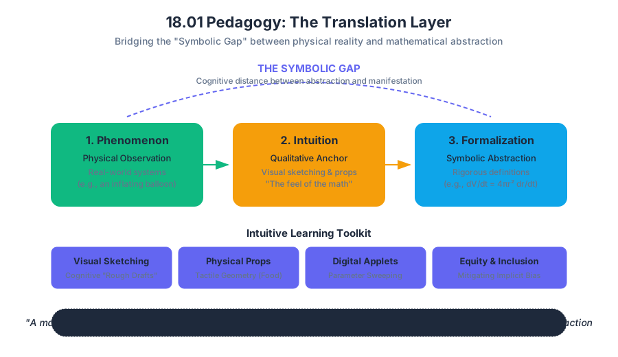
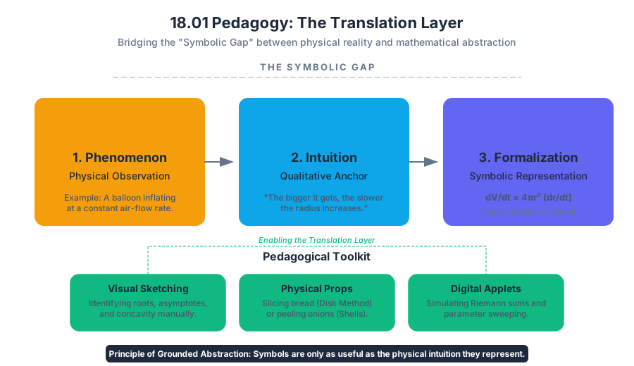
The core mission of this pedagogy is to bridge the Symbolic Gap: the cognitive distance between a mathematical abstraction (e.g., $\int_a^b f(x)dx$) and its physical manifestation (e.g., the total work done by a variable force). By integrating visual sketching, physical props, and digital simulations, the course transforms calculus from a set of rules to be memorized into a toolkit for decoding the physical world.

Mathematical Abstraction vs. Real-World Application

At the heart of the 18.01 philosophy is the tension between Mathematical Abstraction—the pursuit of generalized, symbol-heavy proofs—and Real-World Application—the pragmatic use of calculus to solve engineering and physical problems.

What it is

Abstraction is the process of stripping away the context of a problem to reveal its underlying structure. In calculus, this means moving from "how fast a car is moving" to the derivative $f'(x) = \lim_{h \to 0} \frac{f(x+h) - f(x)}{h}$. While abstraction allows for universal applicability, it can lead to "symbolic alienation," where students manipulate variables without understanding the underlying reality.

Why it matters

Modern STEM education often fails because it introduces abstraction too early, before the student has developed a "physical feel" for the concepts. By grounding every abstract concept in a concrete application, the course ensures that the math remains a "living language."

How it works: The Translation Layer

The pedagogy employs a "Translation Layer" approach, where every new concept is introduced through a three-step pipeline:

1. Phenomenon: A physical observation (e.g., a balloon inflating).
2. Intuition: A qualitative description (e.g., "the bigger it gets, the slower the radius increases for the same amount of air").
3. Formalization: The symbolic representation (e.g., $\frac{dV}{dt} = 4\pi r^2 \frac{dr}{dt}$).

Concept	Abstract Formalism	Real-World Application	Intuitive Anchor
Derivative	$\frac{df}{dx}$	Instantaneous velocity / Marginal cost	The "slope" of a hill at a single point
Integral	$\int f(x)dx$	Total distance / Accumulation of charge	The "sum" of many tiny slices
Limit	$\lim_{x \to a} f(x)$	Convergence of a sequence	Getting "arbitrarily close" to a wall
Optimization	$f'(x) = 0$	Minimizing fuel consumption	Finding the "peak" or "valley"

The Principle of Grounded Abstraction: A mathematical symbol is only as useful as the physical intuition it represents. If a student can solve $\frac{dy}{dx}$ but cannot explain what it means for a cooling cup of coffee, the learning is incomplete.

Intuitive Learning Tools and Visual Sketching

To bridge the gap mentioned above, the course utilizes a suite of Intuitive Learning Tools. These range from low-tech physical props to high-tech digital applets.

Visual Sketching: The "Rough Draft" of Thought

Professor Staffilani emphasizes that sketching is not an artistic endeavor but a cognitive one. When a student sketches a function $f(x)$, they are forced to identify key features:

• Roots: Where does the system "zero out"?
• Asymptotes: Where does the system "break" or reach a limit?
• Concavity: Is the rate of change increasing or decreasing?

Physical Props (The "Food" Method)

One of the most distinctive elements of the 18.01 pedagogy is the use of everyday objects to explain complex geometry.

• Balloons: Used to demonstrate Related Rates. As air is pumped in at a constant rate, the radius grows slower as the balloon gets larger.
• Food (Cakes/Fruit): Used to demonstrate Volumes of Revolution. Slicing a loaf of bread provides a tactile understanding of the Disk Method, while peeling an onion illustrates the Shell Method.

Digital Applets and Simulations

Digital tools allow for "infinite repetition" and "parameter sweeping." A student can slide a bar to see how a Riemann sum approaches an integral as the number of rectangles $n \to \infty$.

import numpy as np
import matplotlib.pyplot as plt

def simulate_riemann_sum(func, a, b, n_rects):
    """
    Low-level implementation of a Riemann Sum visualization logic.
    This mimics the backend of the digital applets used in 18.01.
    """
    x = np.linspace(a, b, n_rects + 1)
    y = func(x)
    
    # Calculate widths and heights
    dx = (b - a) / n_rects
    x_left = x[:-1] # Left endpoints
    y_left = y[:-1]
    
    # The 'Intuitive' part: Summing the areas
    area = np.sum(y_left * dx)
    
    return x_left, y_left, dx, area

# Example usage: f(x) = x^2 from 0 to 2
f = lambda x: x**2
x_coords, y_coords, width, total_area = simulate_riemann_sum(f, 0, 2, 10)

print(f"Calculated Area with 10 rectangles: {total_area}")
# Expected analytical result: 8/3 approx 2.66

Equity and Implicit Bias in STEM

A critical, often overlooked component of the 18.01 pedagogy is the explicit focus on Equity and Implicit Bias. Mathematics has historically been a "gatekeeper" subject, where social pressures and internal biases can discourage talented students from marginalized backgrounds.

Identifying Implicit Bias

Implicit bias refers to the unconscious associations we hold about certain groups. In a STEM classroom, this can manifest as:

• Stereotype Threat: The fear that one will confirm a negative stereotype about their group, which paradoxically hinders performance.
• Participation Gaps: Who feels "authorized" to speak or ask questions in a large lecture hall?

Pedagogical Interventions

Professor Staffilani implements several strategies to mitigate these biases:

1. Diverse Representation: Highlighting the contributions of mathematicians from varied backgrounds.
2. Low-Stakes Testing: Using frequent, low-stakes assessments to reduce the "high-pressure" environment that triggers stereotype threat.
3. Active Learning: Breaking the lecture into small-group problem-solving sessions where every student must contribute.

Bias Type	Manifestation in Calculus	Pedagogical Countermeasure
Stereotype Threat	Student underperforms on high-stakes exams due to anxiety.	Frequent low-stakes quizzes; growth-mindset framing.
Imposter Syndrome	Student feels they "don't belong" at MIT or in STEM.	Explicit discussion of struggle; normalizing failure.
Authority Bias	Only "loud" or "confident" students answer questions.	Random-call systems; anonymous digital polling (e.g., Clickers).
Notation Bias	Students from different curricula struggle with symbols.	Explicitly teaching multiple notations (Leibniz vs. Newton).

The Equity Axiom: Mathematical talent is distributed equally across all demographics, but opportunity and encouragement are not. A successful pedagogy must actively work to rebalance this equation.

Notation Discrepancies across Disciplines

Calculus is the "universal language" of science, but it is spoken in different "dialects." A major hurdle for students is the discrepancy between how a mathematician, a physicist, and an engineer write the same concept.

The Leibniz vs. Newton Conflict

• Mathematicians prefer $f'(x)$ or $Df$ (Lagrange/Euler notation) because it emphasizes the function as an operator.
• Physicists prefer $\frac{dy}{dt}$ (Leibniz notation) because it treats the derivative as a ratio of infinitesimals, which is useful for unit analysis (e.g., meters/second).
• Engineers often use $\dot{y}$ (Newton’s dot notation) for time derivatives to keep equations compact.

Why it Matters: The "Cognitive Load"

When a student moves from a Math lecture to a Physics lab, they often feel they are learning a new subject because the symbols have changed. 18.01 addresses this by explicitly teaching "Notation Fluency."

\begin{aligned}
&\text{Mathematical Form (Operator):} && \frac{d}{dx}[f(x)] \\
&\text{Physical Form (Differential):} && dy = f'(x) dx \\
&\text{Engineering Form (Fluxion):} && \dot{q} = \frac{dq}{dt} \\
&\text{Multivariable Form (Gradient):} && \nabla f
\end{aligned}

Common Pitfalls in Notation

• Treating $dy/dx$ as a fraction: While it behaves like a fraction in many cases (Chain Rule), it is technically a limit. Students often get confused when they can "cancel" the $dx$ in some contexts but not others.
• Variable Confusion: In math, $x$ is the independent variable. In physics, $t$ is usually independent, and $x$ is a dependent variable (position).

Pedagogical Innovation: The "Why" over the "What"

The 18.01 design moves away from the "Cookbook" approach to calculus. In a cookbook approach, students are given a list of recipes (e.g., "To find a maximum, set the derivative to zero"). In the MIT approach, students are asked why the derivative is zero at a peak.

The Mechanics of "Why"

1. Geometric Interpretation: At a peak, the tangent line is horizontal. A horizontal line has a slope of zero.
2. Physical Interpretation: If you throw a ball up, at the very top, its velocity must be zero for an instant before it starts falling.
3. Numerical Interpretation: If $f(x)$ is increasing before $x_0$ and decreasing after $x_0$, it must have passed through zero at $x_0$.

Case Study: Lagrange Multipliers

While a standard course might just give the formula $\nabla f = \lambda \nabla g$, 18.01 explains it through Level Curves. The maximum of a function $f$ subject to a constraint $g$ occurs when the contour lines of $f$ are tangent to the constraint curve $g$. If they weren't tangent, you could keep moving along $g$ to reach a higher contour of $f$.

# Example: Using a CLI tool like 'sympy' to solve an optimization problem
# This demonstrates the 'Real-World' application of the 'Why' philosophy.

python3 -c "
import sympy as sp
x, y, lam = sp.symbols('x y lambda')
f = x**2 + y**2  # Objective: Minimize distance
g = x + y - 1    # Constraint: Must be on the line x+y=1
L = f - lam * g  # Lagrangian
sol = sp.solve([sp.diff(L, x), sp.diff(L, y), sp.diff(L, lam)], [x, y, lam])
print(f'Optimal Point: {sol}')
"

Conclusion: The Holistic Mathematician

The philosophy of 18.01 is that calculus is not a destination, but a lens. By focusing on intuition, visual sketching, and equity, the course aims to produce students who don't just "know" calculus, but who can "think" in calculus. This pedagogical shift ensures that the next generation of engineers and scientists are not just calculators, but thinkers capable of applying abstract logic to the messy, non-linear problems of the real world.

• Symbolic Gap: The cognitive distance between a mathematical formula and its physical meaning.
• Notation Fluency: The ability to translate between different symbolic representations (e.g., Leibniz vs. Newton).
• Stereotype Threat: A psychological phenomenon where fear of confirming a negative stereotype hinders performance.
• Related Rates: A calculus problem type involving finding the rate of change of one quantity based on the rate of change of another.
• Disk Method: A technique for finding the volume of a solid of revolution by "slicing" it into thin cylinders.
• Implicit Bias: Unconscious associations or prejudices toward certain groups of people.
• Concavity: The "bending" of a curve; determined by the second derivative.
• Level Curves: Lines on a graph representing points where a function has a constant value.

1. Which pedagogical tool is best suited for explaining the concept of 'Related Rates' according to Prof. Staffilani?

   • A) A static textbook diagram
   • B) A physical balloon being inflated
   • C) A list of 50 practice problems
   • D) A formal $\epsilon-\delta$ proof Correct: B

2. Why does the course emphasize 'Visual Sketching' over high-precision plotting?

   • A) Because students don't have access to computers.
   • B) Because sketching forces the brain to identify qualitative features like extrema and asymptotes.
   • C) Because it is faster to grade.
   • D) Because sketching is a requirement for the final exam. Correct: B

3. In the context of 'Equity in STEM,' what is 'Stereotype Threat'?

   • A) A bias where teachers favor certain students.
   • B) The fear that one's performance will confirm a negative stereotype about their social group.
   • C) The use of outdated notation in textbooks.
   • D) A physical threat made against students in a classroom. Correct: B

4. Which notation for the derivative is most common in Physics due to its treatment of differentials as ratios?

   • A) $f'(x)$
   • B) $\dot{x}$
   • C) $\frac{dy}{dx}$
   • D) $D_x f$ Correct: C

5. What is the 'Translation Layer' in the 18.01 pedagogy?

   • A) A software tool for translating math into different languages.
   • B) The process of moving from a physical phenomenon to intuition, then to formal symbols.
   • C) A method for converting Celsius to Fahrenheit.
   • D) The way the course is translated for online learners. Correct: B

Core Objectives:

1. Master the "Why": Never accept a formula without understanding its geometric or physical origin.
2. Develop Sketching Habits: Before solving any derivative or integral, draw a rough sketch of the function.
3. Notation Agnosticism: Practice writing the Chain Rule and Product Rule in both $f'(x)$ and $dy/dx$ forms.
4. Identify Bias: Be aware of "Stereotype Threat" and "Imposter Syndrome." Use active learning and low-stakes practice to build confidence.
5. Use the Tools: Engage with digital applets to visualize limits and Riemann sums. Use physical analogies (like the "onion" for shell method) to anchor your spatial reasoning.

Key Formulas to Internalize (Intuition First):

• The Derivative: $f'(x) \approx \frac{\Delta y}{\Delta x}$ (The "Zoom-in" property: any curve looks like a line if you zoom in enough).
• The Integral: $\int f(x)dx \approx \sum f(x_i)\Delta x$ (The "Accumulation" property: adding up tiny contributions to get a whole).
• The Chain Rule: $\frac{dy}{dx} = \frac{dy}{du} \cdot \frac{du}{dx}$ (The "Gears" property: if gear A turns twice as fast as B, and B turns three times as fast as C, A turns six times as fast as C).

Part 1: Differentiation

Differentiation is the cornerstone of modern mathematical analysis, providing the formal framework to quantify change. While algebra allows us to solve for static unknowns, calculus—specifically differentiation—allows us to capture the "dynamic" state of the world. As Professor Gigliola Staffilani (MIT) emphasizes in her approach to 18.01, the transition from average rates of change to instantaneous rates of change is not merely a computational step, but a conceptual leap that bridges the gap between discrete observations and continuous reality.

The Fundamental Definition: The Derivative as a Limit

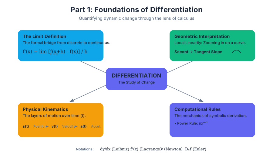
At its core, the derivative of a function measures how the output value changes in response to an infinitesimal change in the input value. We move from the Average Rate of Change (the slope of a secant line connecting two points) to the Instantaneous Rate of Change (the slope of the tangent line at a single point).

The Difference Quotient

To find the slope at a specific point $x$, we consider a second point slightly further away at $x + h$. The slope between these two points is: $$\frac{f(x + h) - f(x)}{h}$$

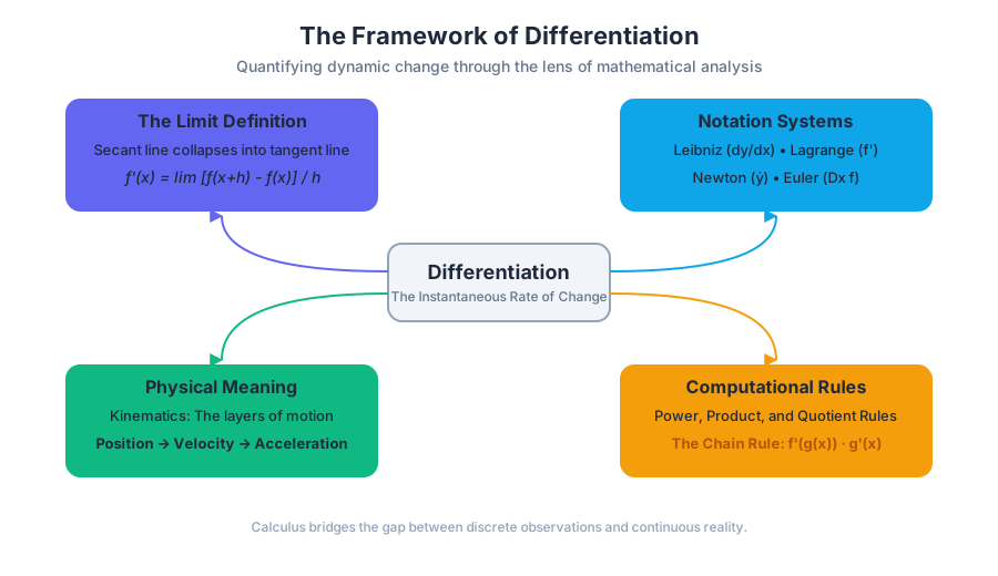
As $h$ approaches zero, this secant line "collapses" into the tangent line. This leads to the formal definition of the derivative, denoted as $f'(x)$ or $\frac{dy}{dx}$:

Definition: The Derivative The derivative of a function $f$ at a point $x$ is defined as: $$f'(x) = \lim_{h \to 0} \frac{f(x + h) - f(x)}{h}$$ provided this limit exists. If the limit exists, the function is said to be differentiable at $x$.

Notation Systems

Differentiation has been refined over centuries, resulting in several notation systems used across different disciplines.

Notation Name	Symbol	Primary Use Case
Leibniz's Notation	$\frac{dy}{dx}$	Calculus, Physics, Differential Equations (emphasizes ratios)
Lagrange's Notation	$f'(x)$	Pure Mathematics, Functional Analysis (emphasizes the function)
Newton's Notation	$\dot{y}$	Physics, Classical Mechanics (specifically for time derivatives)
Euler's Notation	$D_x f$	Linear Algebra, Operator Theory (treats differentiation as an operator)

Geometric Interpretation: The Tangent Line

The most intuitive way to visualize differentiation is through geometry. If you zoom in infinitely on a smooth curve, the curve eventually looks like a straight line. This "local linearity" is the essence of the derivative.

1. The Secant Line: Connects two points $(x, f(x))$ and $(x+h, f(x+h))$. It represents the average speed over an interval.
2. The Tangent Line: Touches the curve at exactly one point, representing the direction the curve is heading at that exact moment.
3. The Slope: The value of the derivative $f'(a)$ is exactly the slope of the tangent line to the graph of $f$ at $x = a$.

The equation of the tangent line at $x = a$ is given by the point-slope form: $$y - f(a) = f'(a)(x - a)$$

Physical Meaning: Kinematics and Beyond

In physics, differentiation translates position into motion. If $s(t)$ represents the position of an object at time $t$, its derivatives reveal the fundamental layers of kinematics.

Derivative Order	Physical Concept	Definition
$s(t)$	Position	Where the object is located in space.
$s'(t) = v(t)$	Velocity	The rate of change of position (speed + direction).
$s''(t) = a(t)$	Acceleration	The rate of change of velocity.
$s'''(t) = j(t)$	Jerk	The rate of change of acceleration (felt as a "jolt").

Worked Example: Falling Objects

Consider an object dropped from a height. Its position is $s(t) = -4.9t^2 + 20$.

• Velocity: $v(t) = s'(t) = -9.8t$. At $t=2$ seconds, the velocity is $-19.6$ m/s (downward).
• Acceleration: $a(t) = v'(t) = -9.8$. This is the constant acceleration due to gravity.

Computational Mechanics: The Rules of the Game

While the limit definition is the theoretical foundation, we use derived rules for efficient computation. These rules allow us to differentiate complex functions by breaking them into smaller, manageable parts.

Fundamental Rules Summary

Rule Name	Mathematical Form	Description
Power Rule	$\frac{d}{dx}[x^n] = nx^{n-1}$	Used for polynomials and radical functions.
Product Rule	$(uv)' = u'v + uv'$	Used when two functions are multiplied.
Quotient Rule	$(\frac{u}{v})' = \frac{u'v - uv'}{v^2}$	Used for ratios of functions.
Chain Rule	$\frac{d}{dx}[f(g(x))] = f'(g(x)) \cdot g'(x)$	Used for nested (composite) functions.

Implementing Numerical Differentiation

In engineering and data science, we often don't have a symbolic formula, only discrete data points. We use numerical methods like the Central Difference Method to approximate the derivative.

import numpy as np

def numerical_derivative(f, x, h=1e-5):
    """
    Computes the numerical derivative of a function f at point x
    using the Central Difference Method, which has an error of O(h^2).
    """
    return (f(x + h) - f(x - h)) / (2 * h)

# Example: f(x) = x^2. Exact derivative at x=3 is 2*3 = 6.
def f(x):
    return x**2

x_val = 3.0
derivative_approx = numerical_derivative(f, x_val)

print(f"Approximated derivative at x={x_val}: {derivative_approx:.10f}")
# Output: Approximated derivative at x=3.0: 6.0000000000

The Chain Rule: The Engine of Deep Learning

The Chain Rule is arguably the most important rule in applied mathematics. It describes how to differentiate a function of a function. If $y$ depends on $u$, and $u$ depends on $x$, then $y$ depends on $x$ through the intermediate variable $u$.

$$\frac{dy}{dx} = \frac{dy}{du} \cdot \frac{du}{dx}$$

This principle is the basis for Backpropagation in neural networks. A neural network is essentially a massive composition of functions; to update weights, we calculate how the final error changes with respect to a weight deep inside the network by "chaining" derivatives backward.

\begin{aligned}
&\text{Let } y = f(g(x)) \\
&\text{Step 1: Identify outer function } f(u) \text{ and inner function } g(x). \\
&\text{Step 2: Differentiate outer: } f'(u). \\
&\text{Step 3: Differentiate inner: } g'(x). \\
&\text{Step 4: Multiply: } f'(g(x)) \cdot g'(x). \\
\\
&\text{Example: } y = \sin(x^2) \\
&u = x^2 \implies \frac{du}{dx} = 2x \\
&y = \sin(u) \implies \frac{dy}{du} = \cos(u) \\
&\frac{dy}{dx} = \cos(x^2) \cdot 2x
\end{aligned}

Automatic Differentiation in Modern Systems

In modern software engineering, we rarely write out derivatives by hand. We use Automatic Differentiation (Autograd). This is distinct from numerical differentiation (which is prone to rounding errors) and symbolic differentiation (which can lead to "expression swell").

Autograd works by tracking the "computational graph" of an operation and applying the chain rule at each node.

import torch

# Define a scalar tensor with gradient tracking enabled
x = torch.tensor(3.0, requires_grad=True)

# Define a complex function: y = (x^2 + 5x) * sin(x)
y = (x**2 + 5*x) * torch.sin(x)

# Compute the derivative dy/dx using Backpropagation
y.backward()

# Access the gradient
print(f"The gradient dy/dx at x=3 is: {x.grad.item()}")
# This computes the exact derivative value using the computational graph.

Pedagogical Philosophy: Bridging the Gap

Professor Staffilani’s teaching philosophy for MIT's 18.01 emphasizes that calculus should not be an "intimidating black box." She advocates for:

1. Visual Intuition: Using applets to show the secant line turning into the tangent line.
2. Physical Props: Using balloons or food items to demonstrate rates of change in volume and surface area.
3. Addressing Bias: Recognizing that the "abstraction gap" often discourages students from underrepresented backgrounds. By grounding differentiation in real-world examples (like the spread of a virus or the optimization of a structural beam), the subject becomes more accessible and equitable.

Common Pitfalls and Misconceptions

• The "h=0" Fallacy: Students often try to plug $h=0$ into the difference quotient immediately. Differentiation is about the limit as $h$ approaches zero, not the value at zero (which would result in $0/0$, an indeterminate form).
• Differentiability vs. Continuity: Every differentiable function is continuous, but not every continuous function is differentiable. A classic example is $f(x) = |x|$ at $x=0$. The "sharp corner" means there is no unique tangent line, so the derivative does not exist there.
• Floating Point Precision: In computational differentiation, choosing an $h$ that is too small can lead to subtractive cancellation errors in standard 64-bit floats.

#include <stdio.h>
#include <math.h>

// Demonstration of precision loss in numerical differentiation
int main() {
    double x = 1.0;
    double exact = cos(1.0); // Derivative of sin(x) is cos(x)
    
    printf("h\t\tError\n");
    printf("------------------------------\n");
    
    for (int i = 1; i <= 16; i++) {
        double h = pow(10, -i);
        double approx = (sin(x + h) - sin(x)) / h;
        double error = fabs(approx - exact);
        printf("1e-%d\t\t%.15e\n", i, error);
    }
    
    return 0;
}
/* 
   Observation: The error decreases until h=1e-8, then increases 
   due to floating point limitations. This is why central 
   difference or Autograd is preferred in production.
*/

Higher-Order Derivatives and Curve Sketching

The first derivative $f'(x)$ tells us if a function is increasing or decreasing. The second derivative $f''(x)$ tells us about the concavity—how the rate of change itself is changing.

• $f'(x) > 0$: Function is increasing.
• $f'(x) < 0$: Function is decreasing.
• $f''(x) > 0$: Concave Up (holds water, like a cup).
• $f''(x) < 0$: Concave Down (sheds water, like a cap).
• $f''(x) = 0$: Potential Inflection Point (where the curve changes concavity).

This hierarchy of derivatives allows engineers to optimize systems—finding the "sweet spot" where a cost function is at its absolute minimum.

• Derivative: The instantaneous rate of change of a function.
• Limit Definition: The formal mathematical foundation of the derivative using $h \to 0$.
• Tangent Line: A straight line that best approximates a curve at a specific point.
• Chain Rule: The formula for the derivative of a composite function: $f'(g(x))g'(x)$.
• Differentiability: The property of a function having a defined derivative at a point.
• Concavity: The "bending" direction of a curve, determined by the second derivative.
• Leibniz Notation: The $\frac{dy}{dx}$ notation emphasizing the ratio of differentials.
• Power Rule: The rule stating that $\frac{d}{dx}x^n = nx^{n-1}$.

1. Conceptual: Why does the derivative of a constant function (e.g., $f(x) = 5$) always equal zero?
   • Answer: A constant function does not change; its rate of change is zero, and its graph is a horizontal line with slope 0.
2. Geometric: If a function has a vertical tangent line at $x=c$, is the function differentiable at $c$?
   • Answer: No. A vertical line has an undefined slope (infinite), so the limit definition of the derivative fails to converge to a real number.
3. Application: You are designing a cooling system where the temperature $T(t)$ drops over time. If $T'(t)$ is negative and $T''(t)$ is positive, what is happening to the cooling rate?
   • Answer: The temperature is decreasing ($T' < 0$), but it is decreasing at a slower and slower rate ($T'' > 0$), suggesting the temperature is stabilizing.
4. Computational: Use the power rule and chain rule to find the derivative of $f(x) = (3x^2 + 1)^4$.
   • Answer: $f'(x) = 4(3x^2 + 1)^3 \cdot (6x) = 24x(3x^2 + 1)^3$.
5. Edge Case: Is the function $f(x) = x^{1/3}$ differentiable at $x=0$?
   • Answer: No. The derivative $f'(x) = \frac{1}{3}x^{-2/3}$ involves division by zero at $x=0$, corresponding to a vertical tangent.

Key Objectives

• Master the limit definition to understand the "why" behind the "how."
• Memorize the fundamental rules (Power, Product, Quotient, Chain) for rapid calculation.
• Connect the derivative to the slope of the tangent line and physical velocity.
• Understand the importance of the Chain Rule in modern computational contexts like AI.
• Recognize the conditions for differentiability (smoothness and continuity).

Practice Problems

1. Derive the derivative of $f(x) = x^2$ using the limit definition.
2. Find the equation of the tangent line to $y = e^x$ at $x = 0$.
3. A particle moves according to $s(t) = t^3 - 6t^2 + 9t$. Find the times when the particle is at rest ($v=0$).
4. Differentiate $y = \ln(\cos(x))$ using the chain rule.

Part 2: Integration

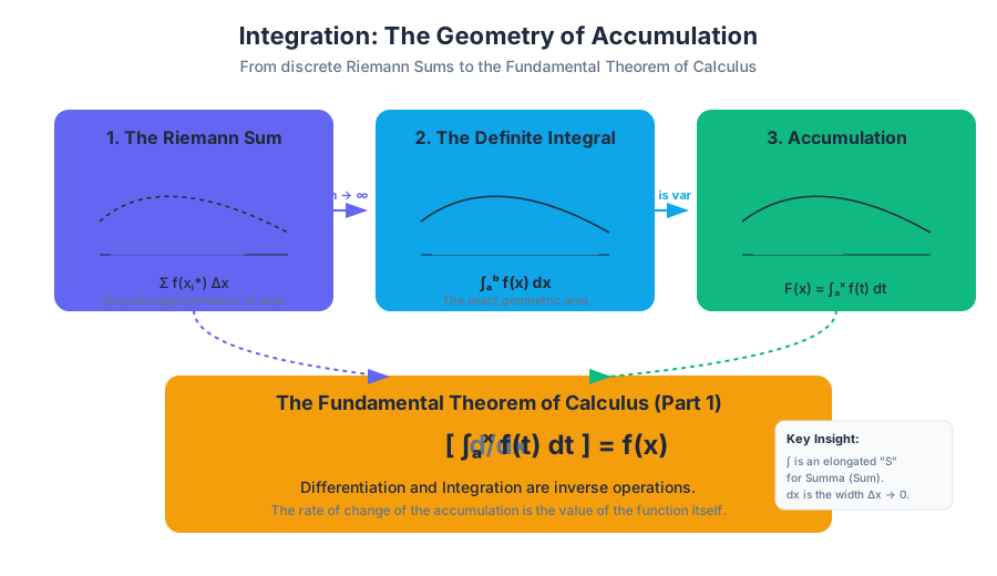
Integration is often introduced as the "inverse" of differentiation, but this characterization, while technically true, undersells its profound conceptual depth. If differentiation is the study of local change—the "instantaneous" snapshot of a system—then integration is the study of accumulation. It is the mathematical machinery that allows us to reconstruct the whole from its infinitesimal parts.

In the pedagogical tradition of MIT’s 18.01, as championed by Professor Gigliola Staffilani, integration is not merely a set of algorithmic procedures (like the Power Rule in reverse). Instead, it is approached as a bridge between the abstract and the tangible. By using visual tools, physical props, and digital applets, we move from the "black box" of the integral symbol $\int$ to a deep understanding of how quantities like area, volume, work, and probability are built from the ground up.

The Definite Integral: The Geometry of Accumulation

The formal journey into integration begins with the Area Problem: how do we calculate the area under a curve $f(x)$ between two points $a$ and $b$? While Euclidean geometry gives us formulas for squares and circles, it fails for the arbitrary, fluctuating curves of the real world.

The Riemann Sum

The solution lies in the Riemann Sum. We partition the interval $[a, b]$ into $n$ sub-intervals of width $\Delta x = \frac{b-a}{n}$. Within each sub-interval, we pick a sample point $x_i^$ and construct a rectangle with height $f(x_i^)$. The total area is approximated by the sum of these rectangles:

$$S_n = \sum_{i=1}^{n} f(x_i^*) \Delta x$$

As $n \to \infty$ (and $\Delta x \to 0$), this sum converges to the Definite Integral:

$$\int_{a}^{b} f(x) , dx = \lim_{n \to \infty} \sum_{i=1}^{n} f(x_i^*) \Delta x$$

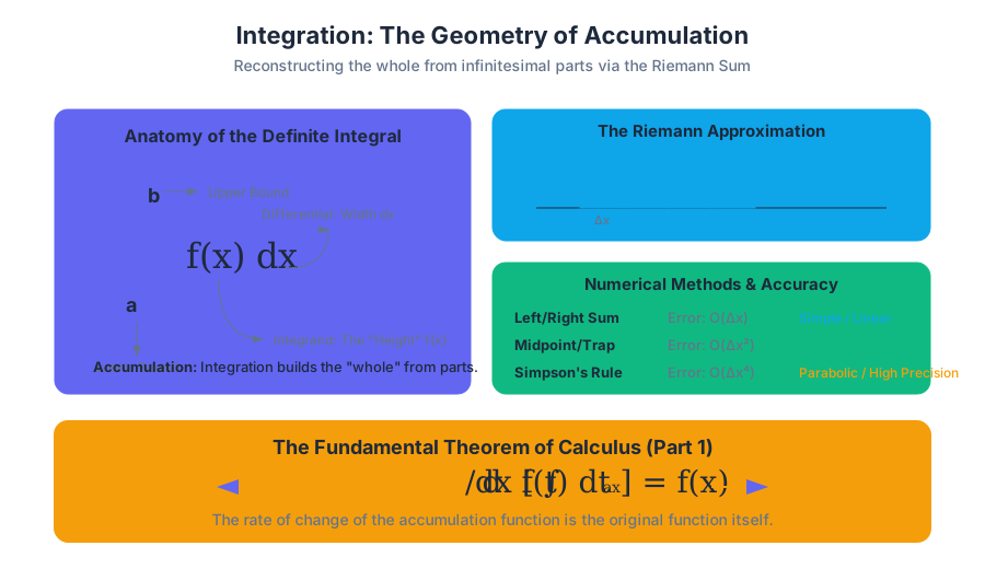
Key Insight: The $dx$ in the integral notation is not just a decorative tag; it represents the infinitesimal width of the rectangles, while $f(x)$ represents the height. The integral sign $\int$ is an elongated "S," standing for summa (sum).

Comparison of Approximation Methods

Depending on where we choose $x_i^*$ (the sample point), the accuracy of our finite sum varies significantly.

Method	Selection of $x_i^*$	Error Characteristic	Best Use Case
Left Riemann Sum	Left endpoint of sub-interval	$O(\Delta x)$; Overestimates if $f$ is decreasing	Quick manual approximations
Right Riemann Sum	Right endpoint of sub-interval	$O(\Delta x)$; Overestimates if $f$ is increasing	Theoretical proofs
Midpoint Rule	Center of sub-interval	$O(\Delta x^2)$; Much more accurate than L/R	General numerical integration
Trapezoidal Rule	Average of endpoints	$O(\Delta x^2)$; Connects points with lines	Data sets with discrete points
Simpson's Rule	Parabolic fit over two intervals	$O(\Delta x^4)$; Extremely high precision	Scientific computing / Engineering

Implementation: Numerical Integration in Python

To see the Riemann Sum in action, we can implement a flexible integrator that demonstrates how increasing $n$ leads to convergence.

import numpy as np

def riemann_sum(f, a, b, n, method='midpoint'):
    """
    Computes the Riemann Sum of function f from a to b with n sub-intervals.
    
    Methods supported: 'left', 'right', 'midpoint'
    """
    dx = (b - a) / n
    
    if method == 'left':
        x = np.linspace(a, b - dx, n)
    elif method == 'right':
        x = np.linspace(a + dx, b, n)
    elif method == 'midpoint':
        x = np.linspace(a + dx/2, b - dx/2, n)
    else:
        raise ValueError("Method must be 'left', 'right', or 'midpoint'")
        
    return np.sum(f(x) * dx)

# Example: Integrate f(x) = x^2 from 0 to 1 (Exact answer is 1/3)
f = lambda x: x**2
for n in [10, 100, 1000]:
    val = riemann_sum(f, 0, 1, n)
    print(f"n={n:4d} | Estimate: {val:.6f} | Error: {abs(1/3 - val):.6e}")

The Accumulation Function

Before we can link integration to differentiation, we must understand the Accumulation Function, denoted as $F(x)$. This function represents the "area so far" as we move from a fixed starting point $a$ to a variable point $x$.

$$F(x) = \int_{a}^{x} f(t) , dt$$

The Dummy Variable

A common point of confusion for students is the introduction of $t$. In the expression above, $x$ is the independent variable of $F$, defining the right-hand boundary of the area. $t$ is a dummy variable—a placeholder that "sweeps" across the interval $[a, x]$.

Physical Intuition

Think of $f(t)$ as the rate of water flowing into a tank (liters per second). $F(x)$ is the total volume of water in the tank at time $x$. If the flow rate $f(t)$ is high, the volume $F(x)$ increases rapidly. If $f(t)$ is zero, the volume $F(x)$ stays constant.

The Fundamental Theorem of Calculus (FTC)

The FTC is the "Great Unification" of calculus. It bridges the gap between the geometry of areas (integration) and the physics of motion (differentiation). It consists of two parts.

FTC Part 1: The Derivative of an Integral

FTC Part 1 states that if $f$ is continuous, then the accumulation function $F(x)$ is the antiderivative of $f(x)$.

$$\frac{d}{dx} \left[ \int_{a}^{x} f(t) , dt \right] = f(x)$$

This tells us that differentiation and integration are inverse operations. If you accumulate a rate of change and then look at the rate at which that accumulation is growing, you get back to the original rate.

Derivation of FTC Part 1

We use the limit definition of the derivative on the accumulation function $F(x)$:

\begin{aligned}
F'(x) &= \lim_{h \to 0} \frac{F(x+h) - F(x)}{h} \\
&= \lim_{h \to 0} \frac{1}{h} \left[ \int_{a}^{x+h} f(t)dt - \int_{a}^{x} f(t)dt \right] \\
&= \lim_{h \to 0} \frac{1}{h} \int_{x}^{x+h} f(t)dt
\end{aligned}

By the Mean Value Theorem for Integrals, there exists a $c$ in $[x, x+h]$ such that $\int_{x}^{x+h} f(t)dt = f(c) \cdot h$. Substituting this in:

$$F'(x) = \lim_{h \to 0} \frac{f(c) \cdot h}{h} = \lim_{h \to 0} f(c)$$

As $h \to 0$, $c$ is forced to $x$. Since $f$ is continuous, $f(c) \to f(x)$. Thus, $F'(x) = f(x)$.

FTC Part 2: The Evaluation Theorem

FTC Part 2 provides the practical tool for calculating definite integrals without resorting to limits of sums.

$$\int_{a}^{b} f(x) , dx = F(b) - F(a)$$

where $F$ is any antiderivative of $f$ (i.e., $F' = f$).

Techniques of Integration: The Toolbelt

While differentiation is largely mechanical (follow the rules), integration is an art form. It often requires pattern recognition and strategic transformations.

Technique	Mathematical Form	Logic / Motivation
Substitution ($u$-sub)	$\int f(g(x))g'(x)dx = \int f(u)du$	The "Chain Rule" in reverse; simplifies compositions.
Integration by Parts	$\int u , dv = uv - \int v , du$	The "Product Rule" in reverse; useful for products of functions ($x e^x$, $x \sin x$).
Partial Fractions	$\frac{P(x)}{Q(x)} = \sum \frac{A_i}{x - r_i}$	Breaks complex rational functions into simple logs/arctans.
Trig Substitution	$x = a \sin \theta$	Uses Pythagorean identities to eliminate square roots ($\sqrt{a^2 - x^2}$).

High-Performance Implementation: Trapezoidal Rule in C

For systems-level engineering or real-time signal processing, we often implement integration in C for maximum throughput.

#include <stdio.h>

// The function we want to integrate
double f(double x) {
    return x * x;
}

/**
 * High-performance Trapezoidal Integration
 * @param a Start point
 * @param b End point
 * @param n Number of steps
 * @return The approximate integral
 */
double integrate_trapezoidal(double a, double b, int n) {
    double h = (b - a) / n;
    double sum = 0.5 * (f(a) + f(b));
    
    for (int i = 1; i < n; i++) {
        sum += f(a + i * h);
    }
    
    return sum * h;
}

int main() {
    double result = integrate_trapezoidal(0.0, 1.0, 1000000);
    printf("Integral of x^2 from 0 to 1: %f\n", result);
    return 0;
}

Real-World Applications: Beyond the Area

Integration is the language of physics and engineering. It allows us to move from "rates" to "totals" across various domains.

1. Physics: Work and Energy

Work is defined as the integral of force over a displacement. If a force $F(x)$ varies as an object moves from $a$ to $b$: $$W = \int_{a}^{b} F(x) , dx$$ This is essential for calculating the energy required to launch a rocket, where gravity weakens as distance increases.

2. Geometry: Volumes of Revolution

By integrating the cross-sectional area of a solid, we can find its volume. Using the Disk Method, the volume of a solid formed by rotating $f(x)$ around the x-axis is: $$V = \pi \int_{a}^{b} [f(x)]^2 , dx$$

3. Data Science: Probability Density

In statistics, the probability that a continuous random variable $X$ falls between $a$ and $b$ is the integral of its probability density function (PDF): $$P(a \le X \le b) = \int_{a}^{b} f(x) , dx$$

Comparison of Physical Interpretations

If $f(x)$ represents...	Then $\int f(x) dx$ represents...
Velocity $v(t)$	Displacement $s(t)$
Acceleration $a(t)$	Change in Velocity $\Delta v$
Power $P(t)$	Energy $E$
Linear Density $\lambda(x)$	Total Mass $M$
Marginal Cost $MC(q)$	Total Variable Cost $TVC$

Pedagogy, Equity, and Intuition

Professor Staffilani emphasizes that the "intimidation factor" of calculus often stems from its abstraction. In the MIT 18.01 curriculum, integration is taught with an eye toward Equity and Implicit Bias.

Bridging the Gap

Many students enter calculus with a "procedural" bias—they believe math is about memorizing steps. This creates a barrier for those who didn't attend elite secondary schools. To counter this, the course uses:

1. Visual Sketching: Encouraging students to draw the "slices" of an integral before writing the formula.
2. Physical Props: Using items like loaves of bread to explain the "Slicing Method" for volumes.
3. Digital Applets: Allowing students to interactively manipulate $n$ in a Riemann sum to see the error shrink.

Common Pitfalls in Integration

Even senior engineers make mistakes when the context shifts.

Pitfall	Description	Consequence
Forgetting $+ C$	Omitting the constant of integration in indefinite integrals.	Loss of a family of solutions; incorrect initial value problems.
Improper Integrals	Integrating over a vertical asymptote without taking limits.	Calculating a finite area for an infinite "hole."
Variable Mismatch	Confusing the variable of integration with a parameter.	Treating $x$ as a constant when it is the independent variable.
Substitution Bounds	Failing to update the limits of integration ($a, b$) when performing $u$-substitution.	Calculating the area in the wrong coordinate space.

Symbolic Integration: Using SymPy

In modern workflows, we often use symbolic engines to handle the heavy lifting of complex antiderivatives.

import sympy as sp

# Define symbols
x, a, b = sp.symbols('x a b')

# Define a complex function: x * exp(-x) * sin(x)
f = x * sp.exp(-x) * sp.sin(x)

# Perform indefinite integration
indefinite = sp.integrate(f, x)
print(f"Indefinite Integral: {indefinite}")

# Perform definite integration from 0 to infinity
definite = sp.integrate(f, (x, 0, sp.oo))
print(f"Definite Integral (0 to inf): {definite}")

Part 3: Coordinate Systems & Infinite Series

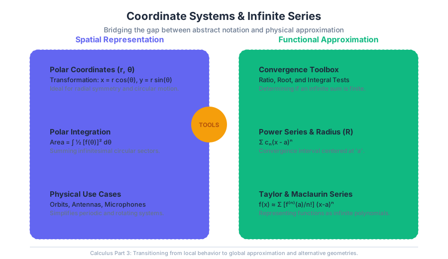
The transition from the calculus of functions in Cartesian space to the study of infinite series and alternative coordinate systems represents a fundamental shift in mathematical maturity. In the previous sections, we focused on the local behavior of functions (derivatives) and the accumulation of quantities (integrals). In Part 3, we address the approximation of reality. As Professor Gigliola Staffilani emphasizes in MIT’s 18.01 curriculum, the goal is to bridge the gap between abstract notation and intuitive physical meaning. Whether we are describing the spiral path of a particle in a magnetic field or approximating a transcendental function for a microprocessor, the tools of coordinate transformation and series expansion are indispensable.

Coordinate Systems: Beyond the Grid

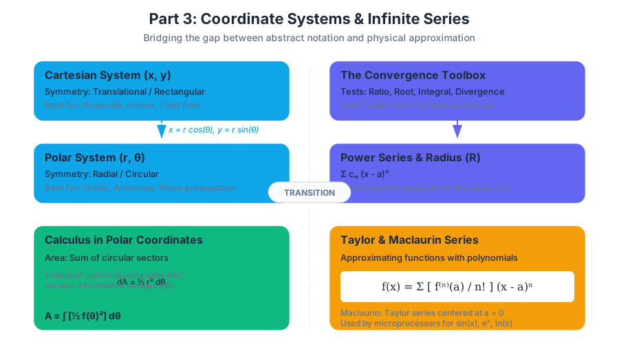
While the Cartesian (rectangular) coordinate system is the bedrock of Euclidean geometry, it is often the most difficult system to use when describing natural phenomena. Circular motion, planetary orbits, and wave propagation often possess radial symmetry that makes $x$ and $y$ coordinates cumbersome.

Polar Coordinates

In a Polar Coordinate System, a point $P$ in the plane is determined by a distance $r$ from a fixed point $O$ (the pole/origin) and an angle $\theta$ from a fixed ray (the polar axis).

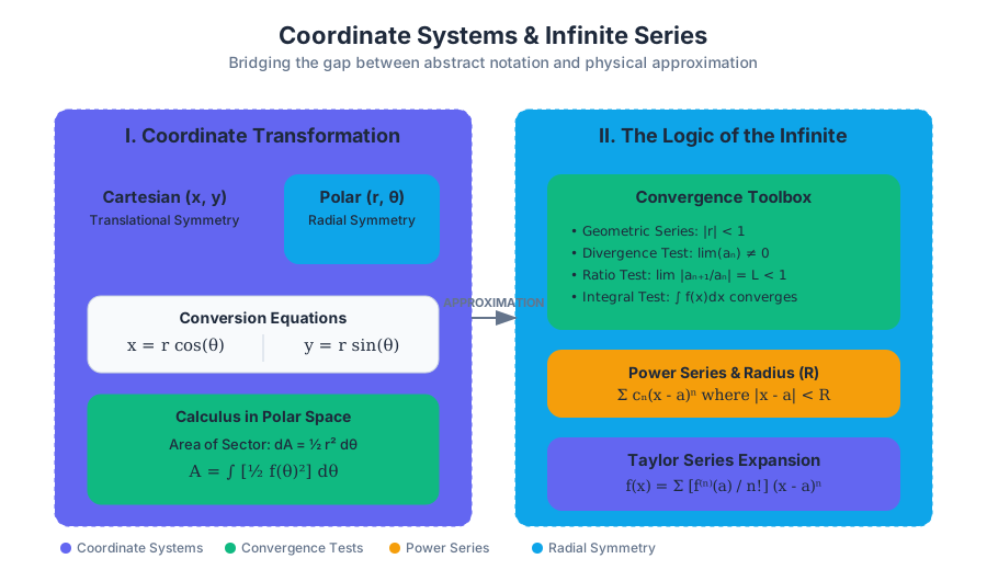
Definition: The relationship between Cartesian coordinates $(x, y)$ and Polar coordinates $(r, \theta)$ is defined by the transformation equations: $$x = r \cos(\theta)$$ $$y = r \sin(\theta)$$ Where $r^2 = x^2 + y^2$ and $\tan(\theta) = y/x$.

Why Polar Coordinates Matter

In engineering and physics, polar coordinates simplify the equations of motion for rotating systems. For instance, the equation of a circle with radius $a$ centered at the origin is the complex $x^2 + y^2 = a^2$ in Cartesian terms, but simply $r = a$ in polar terms.

Feature	Cartesian $(x, y)$	Polar $(r, \theta)$
Symmetry	Translational / Rectangular	Radial / Circular
Grid Lines	Straight lines ($x=c, y=c$)	Concentric circles ($r=c$), Rays ($\theta=c$)
Best Use Case	Projectile motion, Fluid flow in pipes	Orbits, Microphones (Polar patterns), Antennas
Complexity	High for curves (square roots)	Low for periodic/circular functions

Calculus in Polar Coordinates: Area and Arc Length

To find the area $A$ of a region bounded by a polar curve $r = f(\theta)$, we do not use rectangles. Instead, we sum the areas of infinitesimal circular sectors.

The area of a sector is given by $dA = \frac{1}{2}r^2 d\theta$. Thus, the total area is: $$A = \int_{\alpha}^{\beta} \frac{1}{2} [f(\theta)]^2 d\theta$$

Infinite Series: The Logic of the Infinite

An Infinite Series is the sum of the terms of an infinite sequence. The central question of series calculus is not "What is the sum?" but rather "Does the sum exist?" (Convergence vs. Divergence).

Convergence and Divergence

A series $\sum_{n=1}^{\infty} a_n$ converges to a sum $S$ if the sequence of its partial sums $S_k = \sum_{n=1}^{k} a_n$ approaches $S$ as $k \to \infty$. If the partial sums do not approach a finite limit, the series diverges.

The Convergence Toolbox

Determining convergence requires a suite of tests. Choosing the right test is a matter of pattern recognition.

Test Name	Condition for Convergence	Common Use Case
Geometric Series	$\vert r\vert < 1$ for $\sum ar^n$	Fractal geometry, Zeno's paradox
Divergence Test	If $\lim_{n \to \infty} a_n \neq 0$, it diverges	Quick first check for any series
Integral Test	$\int_{1}^{\infty} f(x) dx$ converges	$p$-series, logarithmic series
Ratio Test	$\lim_{n \to \infty} \vert \frac{a_{n+1}}{a_n}\vert < 1$	Power series, factorials, exponentials
Root Test	$\lim_{n \to \infty} \sqrt[n]{\vert a_n\vert } < 1$	Terms raised to the $n$-th power

The Ratio Test: The Engineer's Favorite

The Ratio Test is arguably the most powerful tool for power series. It measures the "growth rate" of terms. If the terms shrink fast enough (faster than a geometric series), the sum is finite.

\text{Given } \sum a_n, \text{ calculate } L = \lim_{n \to \infty} \left| \frac{a_{n+1}}{a_n} \right|
\begin{cases} 
L < 1 & \text{Absolutely Convergent} \\
L > 1 & \text{Divergent} \\
L = 1 & \text{Inconclusive (Try Integral Test)} 
\end{cases}

Power Series and the Radius of Convergence

A Power Series is a series of the form: $$\sum_{n=0}^{\infty} c_n (x - a)^n = c_0 + c_1(x-a) + c_2(x-a)^2 + \dots$$ This is essentially an "infinite polynomial" centered at $a$. Unlike a standard series, a power series may converge for some values of $x$ and diverge for others.

The Radius of Convergence ($R$)

Every power series has a Radius of Convergence $R$.

1. The series converges only when $x = a$ ($R=0$).
2. The series converges for all $x$ ($R=\infty$).
3. The series converges for $|x - a| < R$ and diverges for $|x - a| > R$.

The behavior at the endpoints ($x = a-R$ and $x = a+R$) must be checked separately using other convergence tests.

Taylor and Maclaurin Series

The pinnacle of single-variable calculus is the Taylor Series. It allows us to represent any infinitely differentiable function as a power series. This is how calculators compute $\sin(1.5)$ or $\ln(2)$; they don't look up a table, they calculate a polynomial approximation.

The General Formula

The Taylor series for a function $f(x)$ centered at $a$ is: $$f(x) = \sum_{n=0}^{\infty} \frac{f^{(n)}(a)}{n!} (x - a)^n$$ If $a=0$, the series is specifically called a Maclaurin Series.

Theorem (Taylor’s Theorem): If $f(x)$ is approximated by its $n$-th degree Taylor polynomial $P_n(x)$, the remainder (error) $R_n(x) = f(x) - P_n(x)$ is given by: $$R_n(x) = \frac{f^{(n+1)}(c)}{(n+1)!} (x - a)^{n+1}$$ for some $c$ between $a$ and $x$. This allows us to bound the error of our approximation.

Common Maclaurin Series

These series are the "building blocks" of mathematical analysis.

Function	Series Expansion	Interval of Convergence
$e^x$	$1 + x + \frac{x^2}{2!} + \frac{x^3}{3!} + \dots$	$(-\infty, \infty)$
$\sin x$	$x - \frac{x^3}{3!} + \frac{x^5}{5!} - \dots$	$(-\infty, \infty)$
$\cos x$	$1 - \frac{x^2}{2!} + \frac{x^4}{4!} - \dots$	$(-\infty, \infty)$
$\frac{1}{1-x}$	$1 + x + x^2 + x^3 + \dots$	$(-1, 1)$

Implementation: Computing Sine via Taylor Series

In low-level systems programming, we often avoid standard library math functions for performance or to minimize dependencies. Below is a C implementation of the sine function using a Taylor expansion.

#include <stdio.h>

/**
 * Computes sin(x) using the Maclaurin series:
 * sin(x) = x - x^3/3! + x^5/5! - x^7/7! + ...
 * 
 * This implementation uses an iterative approach to avoid 
 * redundant factorial and power calculations.
 */
double custom_sin(double x, int terms) {
    double term = x;  // First term of the series
    double sum = x;
    double x_squared = x * x;

    for (int i = 1; i < terms; i++) {
        // Each subsequent term is: 
        // prev_term * (-1) * x^2 / ((2i) * (2i + 1))
        term *= -x_squared / ((2 * i) * (2 * i + 1));
        sum += term;
    }
    return sum;
}

int main() {
    double val = 3.1415926535 / 4; // PI/4
    printf("Taylor sin(PI/4) with 5 terms: %.10f\n", custom_sin(val, 5));
    return 0;
}

Real-World Application: Small Angle Approximation

In physics and structural engineering, Taylor series are used to simplify differential equations. For small oscillations (like a pendulum), we use the first term of the Taylor series for $\sin \theta$: $$\sin \theta \approx \theta$$ This turns a non-linear differential equation into a linear one, which is solvable by hand. This "linearization" is the foundation of control theory and stability analysis.

Numerical Verification in Python

Using numpy and scipy, we can visualize how the Taylor polynomial converges to the actual function as we add more terms.

import numpy as np
import matplotlib.pyplot as plt

def taylor_sin(x, n_terms):
    """Compute Taylor series for sin(x) centered at 0."""
    y = np.zeros_like(x)
    for i in range(n_terms):
        sign = (-1)**i
        fact = np.math.factorial(2*i + 1)
        y += sign * (x**(2*i + 1)) / fact
    return y

x_vals = np.linspace(-2*np.pi, 2*np.pi, 1000)
plt.plot(x_vals, np.sin(x_vals), label='Actual sin(x)', lw=3, color='black')

for n in [1, 2, 3, 5]:
    plt.plot(x_vals, taylor_sin(x_vals, n), label=f'n={n} terms')

plt.ylim(-2, 2)
plt.legend()
plt.title("Taylor Approximation Convergence")
plt.show()

Common Pitfalls and Misconceptions

1. Ignoring the Interval of Convergence: A common mistake is using a Taylor series outside its radius of convergence. For example, the series for $\ln(1+x)$ only converges for $-1 < x \leq 1$. Trying to calculate $\ln(5)$ using this series directly will result in divergence.
2. Confusing Sequences and Series: A sequence is a list ($a_1, a_2, \dots$); a series is a sum ($a_1 + a_2 + \dots$). A sequence can converge to zero while its series diverges (e.g., the Harmonic Series $\sum 1/n$).
3. Polar Coordinate Ambiguity: Unlike Cartesian coordinates, polar coordinates are not unique. The point $(1, \pi)$ is the same as $(-1, 0)$ and $(1, 3\pi)$. This "multi-valued" nature can lead to errors when setting integration limits.
4. The "Divergence Test" Fallacy: If $\lim a_n = 0$, the series might converge. It is not a guarantee. The Harmonic Series is the classic counter-example.

Pedagogical Insight: Visualizing the Abstract

Professor Staffilani’s approach to these topics emphasizes that "math is not just symbols on a page." When teaching polar coordinates, she often uses physical props—like a balloon being inflated—to show how radial growth ($dr$) relates to the surface area. For infinite series, she bridges the gap by relating them to digital signals: every digital audio file is essentially a series of approximations (Fourier Series, a relative of Taylor Series) that our ears perceive as continuous sound.

By moving from the rigid grid of Descartes to the fluid rotations of Polar space, and from the exactness of closed-form functions to the flexible power of infinite series, we gain the ability to model the complex, the non-linear, and the infinite.