Backpropagation

Historical Context and the Backwards Method

Overview

The development of backpropagation was not a linear path. While today it is the undisputed engine of the deep learning revolution, its history is a complex tapestry of independent discovery, academic suppression, and cross-disciplinary synthesis. This section examines the historical sociology of neural network research and the early mathematical breakthroughs—specifically the transition from forward sensitivity analysis to the "Backwards Method"—that preceded the modern era.

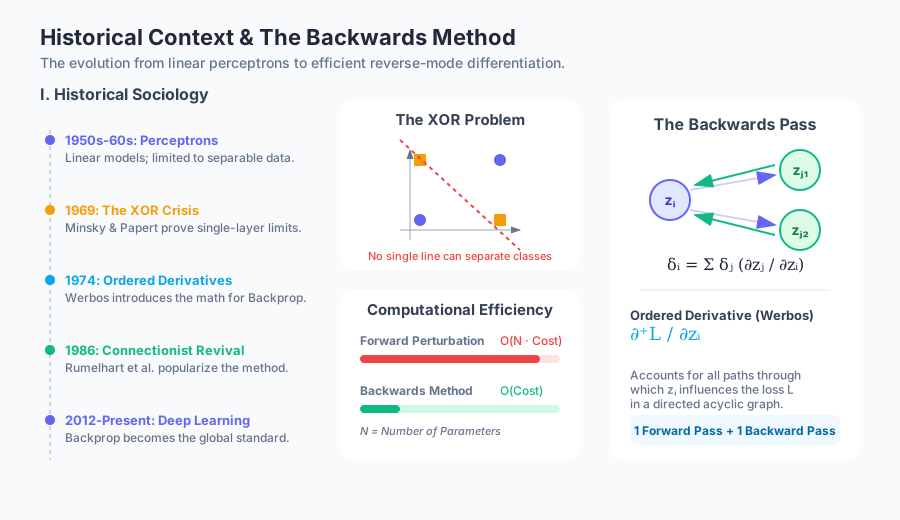
AI_SVGI_SVG## The Historical Sociology of Neural Networks To understand why the "Backwards Method" was revolutionary, one must first understand the intellectual climate of the 1960s and 70s. The field was dominated by Symbolic AI, which viewed intelligence as the manipulation of high-level symbols and logic.

The Perceptron Controversy

In 1958, Frank Rosenblatt introduced the Perceptron, a simple linear classifier. While initially met with fanfare, it was famously critiqued by Marvin Minsky and Seymour Papert in their 1969 book Perceptrons. They mathematically proved that a single-layer perceptron could not solve the XOR problem (non-linearly separable data).

The XOR Problem: A logical operation where the output is true only if the inputs are different. In a 2D plane, the points (0,0) and (1,1) belong to one class, while (0,1) and (1,0) belong to another. No single straight line can separate these two classes.

This critique led to the first "AI Winter," during which funding for connectionist research (neural networks) evaporated. The "Backwards Method" was the key to unlocking multi-layer networks, which could solve XOR, but the mathematical foundations were largely ignored for over a decade.

Era	Dominant Paradigm	Key Limitation	Role of Backprop
1950s-1960s	Perceptrons / Linear Models	Limited to linearly separable data	Non-existent / Early precursors
1970s-1980s	Symbolic AI / Logic	Brittle, "Good Old Fashioned AI" (GOFAI)	Re-discovered (Werbos, Rumelhart)
1990s-2000s	Statistical Learning / SVMs	Feature engineering required	Used in Niche (CNNs, RNNs)
2010s-Present	Deep Learning	Computational cost / Data hungry	Standard optimization engine

---

The Mathematical Foundation: Ordered Derivatives

The breakthrough that eventually became backpropagation was the concept of Ordered Derivatives, introduced by Paul Werbos in his 1974 Harvard Ph.D. thesis. Werbos was not looking for a "brain-like" algorithm; he was looking for a way to improve econometric forecasting and policy modeling.

Definition: Ordered Derivative

An ordered derivative, denoted as $\frac{\partial^+ L}{\partial z_i}$, represents the total change in a target variable $L$ with respect to a variable $z_i$, accounting for all paths through which $z_i$ influences $L$ in a directed acyclic graph (DAG).

Unlike a simple partial derivative $\frac{\partial L}{\partial z_i}$, which assumes all other variables are held constant, the ordered derivative acknowledges that $z_i$ is an input to subsequent variables $z_{i+1}, z_{i+2}, \dots, z_n$.

# Conceptualizing the difference between Partial and Ordered Derivatives
# Let L = f(y, z) where y = g(z)

def partial_derivative_L_wrt_z(z, y):
    # Assumes y is constant
    return d_f / d_z 

def ordered_derivative_L_wrt_z(z):
    # Accounts for the fact that changing z also changes y
    return (d_f / d_z) + (d_f / d_y * d_g / d_z)

---

The Backwards Method (Reverse Mode Differentiation)

The "Backwards Method" is the algorithmic implementation of the chain rule applied in reverse order. In a complex system with $N$ parameters and a single scalar output (the Loss), calculating the gradient via the forward method (perturbing each weight one by one) requires $N$ forward passes. The Backwards Method requires only one forward pass and one backward pass, regardless of the number of parameters.

Why it Matters: Efficiency

The computational complexity of the gradient calculation is the primary bottleneck in training deep models.

Method	Complexity (Time)	Complexity (Memory)	Best Use Case
Forward Perturbation	$O(N \cdot Cost(f))$	$O(1)$	Very few parameters
Symbolic Differentiation	$O(Exp(N))$	$O(Exp(N))$	Simple expressions
Reverse Mode AD (Backprop)	$O(Cost(f))$	$O(N)$	Many parameters, one output

Mechanics of the Backwards Pass

The algorithm operates on a computational graph. For a node $i$ with output $z_i$, the "sensitivity" or "error signal" $\delta_i$ is defined as: $$\delta_i = \frac{\partial L}{\partial z_i}$$

The fundamental recurrence relation for the backwards method is: $$\frac{\partial L}{\partial z_i} = \sum_{j \in \text{Children}(i)} \frac{\partial L}{\partial z_j} \frac{\partial z_j}{\partial z_i}$$

Implementation Example: A Simple 2-Layer MLP

Consider a network where $z_1 = W_1 x$, $a_1 = \sigma(z_1)$, $z_2 = W_2 a_1$, and $L = \frac{1}{2}(y - z_2)^2$.

import numpy as np

def backward_pass(x, y, W1, W2, z1, a1, z2):
    # 1. Compute output error (dL/dz2)
    delta_2 = z2 - y 
    
    # 2. Gradient for W2 (dL/dW2 = dL/dz2 * dz2/dW2)
    # Note: dz2/dW2 is just a1
    grad_W2 = np.outer(delta_2, a1)
    
    # 3. Backpropagate error to hidden layer (dL/da1 = dL/dz2 * dz2/da1)
    # Note: dz2/da1 is W2
    delta_a1 = np.dot(W2.T, delta_2)
    
    # 4. Account for activation function (dL/dz1 = dL/da1 * da1/dz1)
    # Assuming sigmoid: sigma'(z) = sigma(z) * (1 - sigma(z))
    delta_1 = delta_a1 * (a1 * (1 - a1))
    
    # 5. Gradient for W1 (dL/dW1 = dL/dz1 * dz1/dW1)
    grad_W1 = np.outer(delta_1, x)
    
    return grad_W1, grad_W2

---

Backpropagation Through Time (BPTT)

When the "Backwards Method" is applied to sequences, it is known as Backpropagation Through Time (BPTT). This is the standard method for training Recurrent Neural Networks (RNNs).

Network Unfolding

The core insight of BPTT is that a recurrent network (which contains loops) can be "unfolded" into a deep feedforward network where each layer represents a discrete time step. The weights $W$ are shared across all time steps.

Definition: BPTT is the application of the backwards method to a computational graph that has been unrolled over $T$ time steps.

The Gradient Accumulation Problem

Because the same weight matrix $W$ is used at every time step $t$, the total gradient for $W$ is the sum of the gradients calculated at each step: $$\frac{\partial L}{\partial W} = \sum_{t=1}^{T} \frac{\partial L_t}{\partial W}$$

Truncated BPTT

In practice, unfolding a network over thousands of time steps is computationally expensive and leads to the Vanishing Gradient Problem. Truncated BPTT limits the backward pass to a fixed number of steps $k$.

Feature	Standard Backprop	BPTT	Truncated BPTT
Graph Structure	Static DAG	Unrolled Sequence	Fixed-length Window
Weight Sharing	No (usually)	Yes (across time)	Yes (across time)
Memory Usage	$O(\text{Layers})$	$O(\text{Time Steps})$	$O(k)$
Long-term Dependencies	N/A	Theoretical	Limited to $k$

---

Backpropagation Through Structure (BPTS)

Introduced by Goller and Küchler in 1996, Backpropagation Through Structure (BPTS) generalizes BPTT to data that is structured as a tree or a graph rather than a linear sequence.

Recursive Neural Networks

BPTS is used to train Recursive Neural Networks (not to be confused with Recurrent). These are common in Natural Language Processing (NLP) for parsing tree structures or in chemistry for molecular graphs.

1. Forward Pass: The network processes nodes from the leaves up to the root.
2. Backward Pass: The error is propagated from the root down to the leaves.

Mathematical Formulation

For a node $p$ with children $c_1, c_2$: $$h_p = f(W [h_{c1}; h_{c2}] + b)$$ The gradient at node $p$ must be distributed to both $c_1$ and $c_2$ based on the weights $W$ used in the recursive step.

---

Common Pitfalls and Technical Challenges

1. The Vanishing and Exploding Gradient Problem

During the backwards pass, the gradient is multiplied by the weights and the derivative of the activation function at each layer.

• If the weights are small ($<1$) or the derivative is small (e.g., sigmoid saturation), the gradient shrinks exponentially (Vanishing).
• If the weights are large ($>1$), the gradient grows exponentially (Exploding).

2. The "Dead Neuron" Problem

In the backwards method, if an activation function like ReLU outputs 0 for a given input, its derivative is 0. This "kills" the gradient, and the weights for that neuron will never be updated again during that training session.

3. Confusion with Optimization

A common misconception is that backpropagation is the learning algorithm. It is not.

• Backpropagation is only the method for calculating gradients.
• Stochastic Gradient Descent (SGD), Adam, or RMSProp are the optimization algorithms that use those gradients to update the weights.

Concept	Role
Loss Function	Defines the "error" surface.
Backpropagation	Finds the "direction" of steepest ascent/descent.
Optimizer	Decides "how far" to step in that direction.

---

Summary of the "Backwards" Philosophy

The transition from forward-thinking to backward-thinking was a paradigm shift in computational science. By focusing on how the output depends on the internal state (sensitivity) rather than how the input propagates forward (perturbation), researchers unlocked the ability to optimize systems with millions, and now trillions, of parameters.

Whether it is the temporal unfolding of BPTT or the structural recursion of BPTS, the underlying principle remains the same: Dynamic Programming. We store intermediate results (partial derivatives) to avoid redundant calculations, turning an intractable problem into a linear-time operation.

AI_FLASHCARDSI_FLASHCARDS Ordered Derivative: A derivative that accounts for all paths of influence in a system, not just the direct path.

• Reverse Mode AD: The general mathematical name for the backwards method; efficient for functions with many inputs and one output.
• XOR Problem: The classic counter-example that proved single-layer networks were insufficient, necessitating deep networks and backprop.
• Unfolding: The process of transforming a recurrent network into a feedforward one by duplicating layers for each time step.
• Weight Sharing: The technique where the same parameters are used in different parts of the computational graph, requiring gradient summation.
• Sensitivity ($\delta$): The partial derivative of the loss with respect to a specific node's output.

AI_QUIZI_QUIZ. Why is the "Backwards Method" more efficient than the "Forward Method" for neural networks?

• Answer: Because neural networks typically have millions of input parameters (weights) but only one scalar output (Loss). Reverse mode calculates all gradients in one pass, whereas forward mode would require a pass for every single weight.

2. What was the primary contribution of Paul Werbos to this field?

   • Answer: He formalized the concept of "Ordered Derivatives" and reverse-mode differentiation in his 1974 thesis, providing the mathematical framework that would later be called backpropagation.

3. In BPTT, if a sequence has 100 steps, how many times is the weight matrix $W$ updated per sequence?

   • Answer: Once. Although gradients are calculated for each of the 100 steps, they are summed together to perform a single update to the shared weight matrix $W$.

4. What happens to the gradient in BPTS when a node has multiple parents?

   • Answer: The gradients from all parents are summed at that node, following the multivariate chain rule.

5. How does Truncated BPTT mitigate the vanishing gradient problem?

   • Answer: By limiting the number of steps the gradient can flow backward, it prevents the repeated multiplications that cause the gradient to shrink to zero, though at the cost of losing long-term dependency information.

AI_STUDY_GUIDEI_STUDY_GUIDE*Key Equations to Memorize:**

• The Chain Rule: $\frac{dy}{dx} = \frac{dy}{du} \cdot \frac{du}{dx}$
• Error Signal: $\delta_j = \frac{\partial L}{\partial z_j}$
• Weight Update: $w_{ij} \leftarrow w_{ij} - \eta \delta_j a_i$

Historical Timeline:

• 1958: Rosenblatt's Perceptron.
• 1969: Minsky & Papert's Perceptrons (The XOR critique).
• 1974: Werbos's Thesis (Ordered Derivatives).
• 1986: Rumelhart, Hinton, & Williams (Popularization of Backprop).
• 1996: Goller & Küchler (BPTS).

Comparison Checklist:

• Do I understand the difference between a partial derivative and an ordered derivative?
• Can I explain why BPTT requires "unfolding"?
• Do I know the difference between Backpropagation and SGD?
• Can I derive the gradient for a single neuron?

The Core Backpropagation Algorithm

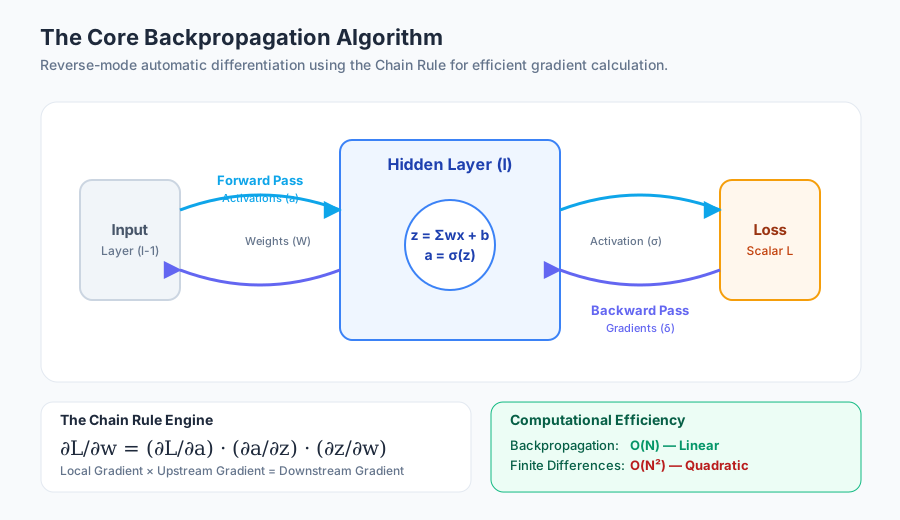
Backpropagation, short for "backward propagation of errors," is the fundamental algorithm that enables the training of deep neural networks. While often conflated with the entire learning process, backpropagation is specifically the method used to calculate the gradient of a loss function with respect to the weights of the network. It is an application of Reverse Mode Automatic Differentiation, leveraging the chain rule from calculus to efficiently assign "credit" (or blame) to each parameter for the final output error.

AI_SVGI_SVG## The Mathematical Foundation: The Chain Rule

At its heart, backpropagation is an exercise in the Chain Rule. In a multi-layer neural network, the output is a nested function of the inputs. If we have a composition of functions $y = f(g(h(x)))$, the derivative of $y$ with respect to $x$ is the product of the derivatives of each component function.

Definition: The Chain Rule If a variable $z$ depends on $y$, which in turn depends on $x$ (i.e., $y = g(x)$ and $z = f(y)$), then $z$ depends on $x$ as well, and the derivative of $z$ with respect to $x$ is given by: $$\frac{dz}{dx} = \frac{dz}{dy} \cdot \frac{dy}{dx}$$

In the context of a neural network, we are interested in $\frac{\partial \mathcal{L}}{\partial w_{ij}^{(l)}}$, where $\mathcal{L}$ is the loss function and $w_{ij}^{(l)}$ is the weight connecting the $i$-th neuron in layer $l-1$ to the $j$-th neuron in layer $l$.

The Local Gradient

Backpropagation works by computing a local gradient at each node. For any given neuron, we calculate how the loss changes with respect to the neuron's output, and then use that to find how the loss changes with respect to the neuron's inputs and parameters.

Component	Symbol	Description
Input	$x$	The raw data or output from the previous layer.
Weight	$w$	The learnable parameter scaling the input.
Bias	$b$	The learnable additive constant.
Pre-activation	$z$	The weighted sum: $z = \sum (w \cdot x) + b$.
Activation	$a$	The non-linear transformation: $a = \sigma(z)$.
Loss	$\mathcal{L}$	The scalar value representing the error.

The Mechanics of the Backward Pass

The training of a neural network consists of two distinct phases: the Forward Pass and the Backward Pass.

1. The Forward Pass

During the forward pass, data flows from the input layer through the hidden layers to the output layer. Each layer performs a linear transformation followed by a non-linear activation.

1. Compute the weighted sum: $z^{(l)} = W^{(l)} a^{(l-1)} + b^{(l)}$
2. Apply activation: $a^{(l)} = \sigma(z^{(l)})$
3. Store intermediate values ($a$ and $z$) for use during the backward pass.

2. The Backward Pass

The backward pass begins at the output layer. We calculate the error gradient and propagate it backward through the network.

1. Compute Output Error: Calculate $\delta^{(L)}$, the gradient of the loss with respect to the pre-activation of the output layer.
2. Propagate Error: For each preceding layer $l = L-1, \dots, 1$, calculate $\delta^{(l)}$ based on $\delta^{(l+1)}$.
3. Compute Parameter Gradients: Use $\delta^{(l)}$ to find the gradients for $W^{(l)}$ and $b^{(l)}$.

Theorem: The Backpropagation Equations For a layer $l$, the error $\delta^{(l)}$ is defined as $\frac{\partial \mathcal{L}}{\partial z^{(l)}}$. The four fundamental equations are:

1. $\delta^{(L)} = \nabla_a \mathcal{L} \odot \sigma'(z^{(L)})$
2. $\delta^{(l)} = ((W^{(l+1)})^T \delta^{(l+1)}) \odot \sigma'(z^{(l)})$
3. $\frac{\partial \mathcal{L}}{\partial b^{(l)}} = \delta^{(l)}$
4. $\frac{\partial \mathcal{L}}{\partial W^{(l)}} = \delta^{(l)} (a^{(l-1)})^T$

Dynamic Programming and Efficiency

One might wonder why we don't simply use symbolic differentiation or finite differences to calculate gradients. The answer lies in computational complexity.

If a network has $N$ parameters, calculating the gradient via finite differences (perturbing each weight slightly and re-running the forward pass) would require $O(N)$ forward passes. For modern models with billions of parameters, this is impossible.

Backpropagation is a Dynamic Programming algorithm. It avoids redundant calculations by caching the intermediate activations during the forward pass and the intermediate gradients during the backward pass. This allows us to compute the gradients for all parameters in a single backward pass, which has a computational cost roughly equivalent to two forward passes.

Method	Complexity	Pros	Cons
Finite Differences	$O(N^2)$	Simple to implement	Extremely slow for large $N$
Symbolic Diff.	Variable	Exact expressions	Can lead to "expression swell"
Backpropagation	$O(N)$	Highly efficient, scales to billions	Requires storing activations (memory intensive)

Implementation: Matrix Calculus and Tensors

In practice, we do not iterate over individual neurons. Instead, we use Matrix Multiplication to process entire layers and batches of data simultaneously. This leverages the highly optimized BLAS (Basic Linear Algebra Subprograms) libraries and GPU architectures.

Python Implementation (NumPy)

The following code demonstrates a single update step for a simple 2-layer MLP.

import numpy as np

def sigmoid(x):
    return 1 / (1 + np.exp(-x))

def sigmoid_derivative(x):
    return sigmoid(x) * (1 - sigmoid(x))

# Hyperparameters and Data
X = np.array([[0, 0], [0, 1], [1, 0], [1, 1]]) # Input
y = np.array([[0], [1], [1], [0]])             # Target (XOR)
learning_rate = 0.1

# Initialize weights
W1 = np.random.randn(2, 4)
b1 = np.zeros((1, 4))
W2 = np.random.randn(4, 1)
b2 = np.zeros((1, 1))

# --- Forward Pass ---
z1 = np.dot(X, W1) + b1
a1 = sigmoid(z1)
z2 = np.dot(a1, W2) + b2
a2 = sigmoid(z2)

# --- Backward Pass ---
# 1. Output layer error
loss_grad = a2 - y # Derivative of MSE loss: (a2 - y)^2
d_z2 = loss_grad * sigmoid_derivative(z2)

# 2. Gradients for W2 and b2
d_W2 = np.dot(a1.T, d_z2)
d_b2 = np.sum(d_z2, axis=0, keepdims=True)

# 3. Hidden layer error
d_a1 = np.dot(d_z2, W2.T)
d_z1 = d_a1 * sigmoid_derivative(z1)

# 4. Gradients for W1 and b1
d_W1 = np.dot(X.T, d_z1)
d_b1 = np.sum(d_z1, axis=0, keepdims=True)

# --- Update Weights ---
W2 -= learning_rate * d_W2
b2 -= learning_rate * d_b2
W1 -= learning_rate * d_W1
b1 -= learning_rate * d_b1

Backpropagation Through Time (BPTT)

Standard backpropagation is designed for feedforward networks. However, Recurrent Neural Networks (RNNs) process sequences by maintaining a hidden state that persists across time steps. To train these, we use Backpropagation Through Time (BPTT).

The Unfolding Concept

BPTT works by "unfolding" the RNN into a deep feedforward network where each layer represents a time step. The critical distinction is that the weights are shared across all time steps.

1. Unfold: Create a copy of the network for each time step in the sequence.
2. Forward Pass: Compute the hidden states and outputs for the entire sequence.
3. Backward Pass: Accumulate gradients for the shared weights across all time steps.
4. Update: Apply the accumulated gradient to the weights.

Truncated BPTT

For very long sequences, standard BPTT suffers from the Vanishing Gradient Problem and high memory usage. Truncated BPTT processes the sequence in smaller chunks (e.g., 20 time steps), stopping the gradient flow after a certain point to maintain stability and efficiency.

Backpropagation Through Structure (BPTS)

While BPTT handles sequences, Backpropagation Through Structure (BPTS) is used for Recursive Neural Networks, which operate on tree-structured data (like parse trees in linguistics or molecular graphs in chemistry).

In BPTS, the topology of the network is determined by the structure of the input data. The gradient is propagated from the root of the tree down to the leaves. This allows the model to learn distributed representations of hierarchical structures.

Algorithm	Network Type	Data Structure	Key Characteristic
Standard Backprop	Feedforward (MLP, CNN)	Fixed-size vectors/images	Direct DAG flow
BPTT	Recurrent (RNN, LSTM)	Sequences (Time)	Weight sharing across time
BPTS	Recursive	Trees/Graphs	Dynamic topology per input

Common Pitfalls and Challenges

Even with a perfect implementation, backpropagation can fail due to the mathematical properties of the network.

1. The Vanishing Gradient Problem

When using activation functions like Sigmoid or Tanh, the derivative is very small for large positive or negative inputs. As we multiply these small derivatives across many layers (via the chain rule), the gradient effectively "vanishes" by the time it reaches the early layers.

• Solution: Use ReLU (Rectified Linear Unit) activations or Batch Normalization.

2. The Exploding Gradient Problem

Conversely, if weights are initialized too large, the gradients can grow exponentially, leading to numerical instability (NaN values).

• Solution: Use Gradient Clipping or careful weight initialization (e.g., Xavier/Glorot or He initialization).

3. Local Optima and Saddle Points

In high-dimensional spaces, the loss surface is complex. While true local minima are rare in deep learning, saddle points (where the gradient is zero but it's not a minimum) are common and can slow down training.

• Solution: Use momentum-based optimizers like Adam or RMSProp.

4. The Dying ReLU

If a ReLU neuron's input is always negative, its gradient becomes zero, and it will never update again—it "dies."

• Solution: Use Leaky ReLU or lower learning rates.

Activation Functions and Their Derivatives

The choice of activation function $\sigma$ is critical because its derivative $\sigma'$ is a direct multiplier in the backpropagation formula.

Activation	Formula $\sigma(x)$	Derivative $\sigma'(x)$	Notes
Sigmoid	$\frac{1}{1+e^{-x}}$	$\sigma(x)(1-\sigma(x))$	Vanishing gradient risk; output not zero-centered.
Tanh	$\frac{e^x - e^{-x}}{e^x + e^{-x}}$	$1 - \sigma(x)^2$	Zero-centered; still prone to vanishing gradients.
ReLU	$\max(0, x)$	$1$ if $x>0$, else $0$	Efficient; solves vanishing gradient; "dying" risk.
Leaky ReLU	$\max(\alpha x, x)$	$1$ if $x>0$, else $\alpha$	Prevents dying neurons by allowing small gradient.

Summary of the Backpropagation Workflow

To summarize the entire process for a single training iteration:

1. Input: Provide a batch of training data $X$.
2. Forward Pass: Compute activations $a^{(l)}$ for every layer.
3. Loss Calculation: Compute the scalar error $\mathcal{L}$ using a loss function (e.g., Cross-Entropy).
4. Output Gradient: Calculate the error signal $\delta^{(L)}$ for the final layer.
5. Backpropagation: Iterate backward from $L-1$ to $1$ to compute $\delta^{(l)}$ for all hidden layers.
6. Weight Gradients: Calculate $\frac{\partial \mathcal{L}}{\partial W}$ and $\frac{\partial \mathcal{L}}{\partial b}$ using the stored activations and error signals.
7. Optimization: Update the weights using an optimizer (SGD, Adam, etc.): $W = W - \eta \nabla_W \mathcal{L}$.

Backpropagation remains the most successful algorithm in the history of AI, providing the mathematical bridge between high-level objectives (the loss function) and low-level parameter adjustments.

AI_STUDY_GUIDEI_STUDY_GUIDE### Flashcards: Backpropagation Essentials

• Q: What is the primary mathematical tool used in backpropagation?
  • A: The Chain Rule.
• Q: Why is backpropagation considered a dynamic programming algorithm?
  • A: Because it stores (caches) intermediate results (activations and gradients) to avoid redundant calculations.
• Q: What is the "error signal" $\delta$ in backpropagation?
  • A: The partial derivative of the loss function with respect to the pre-activation $z$ of a neuron ($\partial \mathcal{L} / \partial z$).
• Q: How does BPTT differ from standard backpropagation?
  • A: BPTT unfolds the network across time steps and accumulates gradients for shared weights.
• Q: What is the main advantage of ReLU over Sigmoid for backpropagation?
  • A: ReLU has a constant gradient of 1 for positive inputs, which helps prevent the vanishing gradient problem.

Quiz: Conceptual Understanding

1. True or False: Backpropagation is an optimization algorithm like Gradient Descent.
   • Answer: False. Backpropagation is a method for calculating gradients; Gradient Descent is an optimization algorithm that uses those gradients.
2. In a network with 10 layers, if the gradient at layer 10 is 0.5 and the derivative of the activation at layer 9 is 0.1, what happens to the error signal as it moves backward?
   • Answer: It is scaled (multiplied) by the activation derivative and the weights, typically becoming smaller (vanishing).
3. Which pass (Forward or Backward) requires more memory, and why?
   • Answer: The Backward pass indirectly requires more memory because it needs the activations stored during the Forward pass to compute gradients.
4. What happens to the weight update if the activation of a neuron is zero?
   • Answer: According to the equation $\frac{\partial \mathcal{L}}{\partial W} = \delta \cdot a^T$, if the activation $a$ is zero, the gradient for the weight $W$ will be zero, and the weight will not update.

Study Guide: Mastering Backpropagation

1. Derive the Chain Rule: Practice deriving the gradient for a single-neuron "network" ($y = \sigma(wx+b)$).
2. Matrix Dimensions: Ensure you can trace the shapes of matrices through the forward and backward pass. If $W$ is $(m, n)$, then $\nabla_W$ must also be $(m, n)$.
3. Activation Derivatives: Memorize the derivatives of Sigmoid, Tanh, and ReLU. They are the "gates" through which the gradient flows.
4. Implementation: Write a backpropagation script from scratch using only NumPy. Do not use PyTorch or TensorFlow until you can do it in raw math.
5. Vanishing Gradient: Visualize the Sigmoid curve and its derivative. Note how the derivative approaches zero at the tails—this is the visual explanation of the vanishing gradient.

Theoretical Derivations and Optimal Control

The evolution of gradient-based learning is often presented as a modern triumph of computer science, yet its roots are deeply embedded in the soil of 1960s optimal control theory and variational calculus. This section explores the rigorous mathematical foundations of backpropagation, its temporal and structural extensions, and its identity as a specific case of discrete-time optimal control.

By framing neural network training through the lens of the Kelley-Bryson optimal-control gradient formula, we move beyond simple "error correction" and into the realm of trajectory optimization. This perspective is vital for engineering systems where the "output" is not merely a classification label, but a sequence of actions in a dynamic environment.

AI_SVGI_SVG## The Fundamental Mechanics of Backpropagation

At its core, Backpropagation is an efficient algorithm for calculating the gradient of a loss function with respect to the weights of a neural network. While often conflated with optimization algorithms like Stochastic Gradient Descent (SGD), backpropagation strictly refers to the computation of the gradient, not the update itself.

1. What it is: Reverse Mode Automatic Differentiation

Mathematically, backpropagation is a specific implementation of Reverse Mode Automatic Differentiation (AD). It leverages the Chain Rule of calculus to propagate the "blame" for the error from the output layer back to the input layer.

Definition: The Backpropagation Principle Given a composite function $L(f_n(...f_1(x)))$, the gradient $\nabla L$ is computed by caching intermediate derivatives during a forward pass and accumulating products in reverse order. This reduces the computational complexity from $O(N^2)$ (for naive finite differences) to $O(N)$, where $N$ is the number of parameters.

2. The Mathematical Derivation

Consider a feedforward network where $a^{(l)}$ is the activation of layer $l$, $w^{(l)}$ are the weights, and $\sigma$ is the activation function. The forward pass is defined as: $$z^{(l)} = w^{(l)} a^{(l-1)} + b^{(l)}$$ $$a^{(l)} = \sigma(z^{(l)})$$

To find the gradient of the loss $C$ with respect to a weight $w_{jk}^{(l)}$, we apply the chain rule: $$\frac{\partial C}{\partial w_{jk}^{(l)}} = \frac{\partial C}{\partial z_j^{(l)}} \frac{\partial z_j^{(l)}}{\partial w_{jk}^{(l)}}$$

We define the error term (or "sensitivity") of node $j$ in layer $l$ as: $$\delta_j^{(l)} = \frac{\partial C}{\partial z_j^{(l)}}$$

The recursive step that defines backpropagation is: $$\delta^{(l)} = ((w^{(l+1)})^T \delta^{(l+1)}) \odot \sigma'(z^{(l)})$$ where $\odot$ denotes the Hadamard (element-wise) product.

Component	Symbol	Role in Derivation
Loss Function	$C$ or $L$	The scalar value we aim to minimize.
Activation	$a^{(l)}$	The output of a layer after the non-linearity.
Pre-activation	$z^{(l)}$	The weighted sum before the non-linearity.
Sensitivity	$\delta^{(l)}$	The partial derivative of loss w.r.t. the pre-activation.
Weight Gradient	$\nabla_w C$	The final product used by the optimizer.

3. Why it Matters: Dynamic Programming

Backpropagation is an application of Dynamic Programming. By storing the sensitivities $\delta^{(l)}$ at each layer, we avoid the redundant re-calculation of the chain rule for every single weight. In a deep network, a weight in the first layer contributes to the error through millions of paths; backpropagation collapses these paths into a single recursive calculation.

4. Implementation Example (Python/NumPy)

The following code demonstrates a non-trivial backward pass for a single dense layer, highlighting the matrix operations that mirror the theoretical derivation.

import numpy as np

def backward_pass(activations, weights, biases, z_values, target, loss_derivative_func):
    """
    Performs a single backward pass for a multi-layer perceptron.
    """
    layers = len(weights)
    deltas = [None] * layers
    grad_w = [None] * layers
    grad_b = [None] * layers
    
    # 1. Compute output error (delta for the last layer)
    # delta^L = grad_a(C) * sigma'(z^L)
    output_activation = activations[-1]
    delta = loss_derivative_func(output_activation, target) * sigmoid_prime(z_values[-1])
    deltas[-1] = delta
    
    # 2. Backpropagate the error
    for l in range(layers - 2, -1, -1):
        # delta^l = (W^{l+1}.T @ delta^{l+1}) * sigma'(z^l)
        delta = np.dot(weights[l+1].T, deltas[l+1]) * sigmoid_prime(z_values[l])
        deltas[l] = delta
        
    # 3. Compute gradients for weights and biases
    for l in range(layers):
        # grad_w = delta^l @ activation^{l-1}.T
        grad_w[l] = np.dot(deltas[l], activations[l].T)
        grad_b[l] = deltas[l]
        
    return grad_w, grad_b

def sigmoid_prime(z):
    """Derivative of the sigmoid function."""
    s = 1 / (1 + np.exp(-z))
    return s * (1 - s)

Optimal Control and the Kelley-Bryson Formula

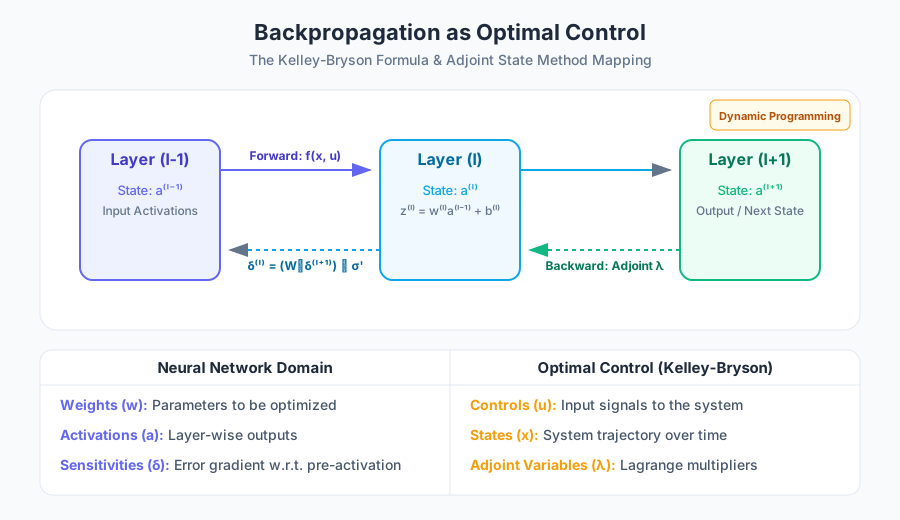
The connection between backpropagation and Optimal Control is found in the Adjoint State Method. In the 1960s, Henry J. Kelley and Arthur E. Bryson developed methods for optimizing the trajectories of rockets. Their work provided the exact mathematical framework that would later be recognized as backpropagation.

1. The Control Perspective

In optimal control, we seek a control sequence $u_t$ that minimizes a cost function $J$ subject to system dynamics $x_{t+1} = f(x_t, u_t)$. If we view a neural network as a discrete-time dynamical system:

• States ($x_t$): The activations of layer $t$.
• Controls ($u_t$): The weights of layer $t$.
• Dynamics ($f$): The layer transformation (linear sum + activation).

2. The Hamiltonian and Adjoint Variables

To solve this, we define the Hamiltonian: $$H_t = L(x_t, u_t) + \lambda_{t+1}^T f(x_t, u_t)$$ where $\lambda$ are the Lagrange Multipliers (or Adjoint Variables). The "Adjoint Equation" describes how these multipliers evolve: $$\lambda_t = \frac{\partial H_t}{\partial x_t} = \frac{\partial f^T}{\partial x_t} \lambda_{t+1} + \frac{\partial L}{\partial x_t}$$

This is precisely the backpropagation formula. The adjoint variables $\lambda$ are the sensitivities $\delta$ we use in machine learning.

Control Theory Term	Neural Network Equivalent
Adjoint State ($\lambda$)	Error Sensitivity ($\delta$)
Plant Dynamics ($f$)	Layer Transformation
Control Input ($u$)	Network Weights ($w$)
Terminal Cost	Loss Function ($C$)
Hamiltonian ($H$)	Local Objective Function

3. Why this matters: Hidden-Node Teaching

By treating the network as a control system, we can implement Hidden-Node Teaching. Instead of only providing a target at the final output, we can treat hidden layers as intermediate states with their own "desired" trajectories. This is used in Target Propagation and helps mitigate the vanishing gradient problem by providing local anchors for learning.

Backpropagation Through Time (BPTT)

When dealing with sequential data, such as speech or time-series, we use Recurrent Neural Networks (RNNs). Training these requires Backpropagation Through Time (BPTT).

1. What it is: Network Unfolding

BPTT works by "unfolding" the recurrent network into a deep feedforward network where each layer represents a time step. The key constraint is Shared Parameters: the same weight matrix $W$ is used at every time step.

2. The Mechanics of BPTT

In an unfolded RNN of $T$ steps, the total loss is the sum of losses at each time step: $L = \sum_{t=1}^T L_t$. The gradient with respect to the shared weights $W$ is the sum of the gradients at each time step: $$\frac{\partial L}{\partial W} = \sum_{t=1}^T \frac{\partial L_t}{\partial W}$$

Because the state $h_t$ depends on $h_{t-1}$, the gradient $\frac{\partial L_t}{\partial W}$ must be computed by backpropagating through all previous time steps: $$\frac{\partial L_t}{\partial W} = \sum_{k=1}^t \frac{\partial L_t}{\partial h_t} \frac{\partial h_t}{\partial h_k} \frac{\partial h_k}{\partial W}$$

3. Variations: Truncated BPTT

For very long sequences (e.g., thousands of words), standard BPTT is computationally expensive and prone to Vanishing/Exploding Gradients. Truncated BPTT processes the sequence in chunks. It performs a forward pass for $n$ steps, but only backpropagates for $k$ steps ($k \le n$).

Method	Memory Complexity	Gradient Accuracy	Use Case
Full BPTT	$O(T)$	Exact	Short sequences, high precision.
Truncated BPTT	$O(k)$	Biased/Approximate	Long sequences (NLP, Audio).
Real-Time Recurrent Learning (RTRL)	$O(N^4)$	Exact (Forward)	Online learning in small networks.

4. Common Pitfalls: The Vanishing Gradient

In BPTT, the term $\frac{\partial h_t}{\partial h_k}$ involves a product of Jacobian matrices: $$\prod_{i=k+1}^t \frac{\partial h_i}{\partial h_{i-1}}$$ If the eigenvalues of the weight matrix are less than 1, the gradient shrinks exponentially as it travels back in time, effectively "forgetting" long-term dependencies. This led to the development of Gated Architectures like LSTM and GRU.

Backpropagation Through Structure (BPTS)

While BPTT handles linear sequences, Backpropagation Through Structure (BPTS) extends gradient-based learning to Recursive Neural Networks, which operate on tree-structured or graph-structured data.

1. What it is: Recursive Learning

BPTS is used when the input is a structure, such as a parse tree in linguistics or a molecular graph in chemistry. Instead of a fixed sequence of time steps, the "unfolding" follows the topology of the input structure.

2. How it Works

1. Structural Forward Pass: The network processes nodes from the leaves up to the root. Each parent node activation is a function of its children: $h_{parent} = f(h_{child1}, h_{child2}, W)$.
2. Structural Backward Pass: The gradient is propagated from the root down to the leaves. At each branching point, the error signal is split and sent to the children according to the weights of the recursive transformation.

3. Distributed Representations

BPTS was pioneered by Goller and Küchler (1996) to learn Task-Dependent Distributed Representations. By training on structures, the network learns to map complex symbolic trees into a continuous vector space where semantic similarity is represented by spatial proximity.

4. Comparison of Backpropagation Variants

Feature	Standard Backprop	BPTT	BPTS
Topology	Fixed DAG (Layers)	Linear Chain (Time)	Tree/Graph (Structure)
Weight Sharing	No (usually)	Across time steps	Across recursive nodes
Primary Application	Image Classification	Speech, Translation	Logic, Chemistry, Parsing
Complexity	$O(Layers)$	$O(Time)$	$O(Nodes)$

Theoretical Challenges and Modern Perspectives

1. The Local Optima Myth

Early critiques of backpropagation focused on the risk of getting stuck in local optima. However, high-dimensional optimization research suggests that in large neural networks, local minima are rarely the problem. Instead, saddle points (where the gradient is zero but the point is not a minimum) are the primary obstacle. Modern optimizers like Adam and RMSProp use momentum to "slide" past these saddle points.

2. Biological Plausibility

A major debate in theoretical neuroscience is whether the brain performs backpropagation. The "Weight Transport Problem" (the need for the backward pass to know the exact weights of the forward pass) makes standard BP biologically unlikely. This has led to theories like Feedback Alignment, where random backward weights can still provide useful gradient signals.

3. Second-Order Methods

While backpropagation provides the first derivative (Jacobian), some researchers use Hessian-Free Optimization or K-FAC (Kronecker-factored Approximate Curvature) to incorporate second-order information. These methods can converge in fewer iterations but require significantly more computation per step.

Key Insight: The Duality of Learning Backpropagation is not just an algorithm; it is a bridge. It connects the discrete world of symbolic logic (through BPTS) and the continuous world of physical dynamics (through Optimal Control). Every time we train a model, we are essentially solving a high-dimensional trajectory optimization problem.

AI_STUDY_GUIDEI_STUDY_GUIDE--

Appendix: Summary of Key Formulas

1. The Adjoint State Equation (Optimal Control): $$\lambda_t = \left( \frac{\partial f}{\partial x_t} \right)^T \lambda_{t+1} + \frac{\partial L}{\partial x_t}$$

2. The BPTT Gradient (RNN): $$\frac{\partial L}{\partial W} = \sum_{t=1}^T \sum_{k=1}^t \frac{\partial L_t}{\partial h_t} \left( \prod_{i=k+1}^t \frac{\partial h_i}{\partial h_{i-1}} \right) \frac{\partial h_k}{\partial W}$$

3. The BPTS Recursive Step: $$\delta_{child} = (W_{branch}^T \delta_{parent}) \odot \sigma'(z_{child})$$

---

This article is part of the DeepWiki series on Neural Computation and Control Theory. For further reading, see the sections on "Variational Calculus in Machine Learning" and "Gated Recurrent Units."

Backpropagation for Specialized Architectures

The fundamental algorithm of modern deep learning, Backpropagation, is often misunderstood as a synonym for learning itself. In reality, it is a specific application of Reverse-Mode Automatic Differentiation (AD) designed to compute the gradient of a scalar loss function with respect to the weights of a neural network. While the standard algorithm suffices for Feedforward Neural Networks (FNNs), it encounters significant theoretical and practical hurdles when applied to architectures with temporal dependencies, structural hierarchies, or shared parameters.

To train models like Recurrent Neural Networks (RNNs) or Recursive Neural Networks, we must adapt the backpropagation algorithm to account for parameter sharing and the topology of the data. This article explores the mathematical foundations and implementation nuances of Backpropagation Through Time (BPTT) and Backpropagation Through Structure (BPTS).

AI_SVGI_SVG## The Mathematical Foundation: Chain Rule and Dynamic Programming

At its core, backpropagation is an exercise in the Chain Rule of calculus, optimized via Dynamic Programming. For a composite function $y = f(g(x))$, the derivative is $\frac{dy}{dx} = \frac{dy}{dg} \cdot \frac{dg}{dx}$. In a neural network, this allows us to propagate the "error signal" from the output layer back to the input.

Theorem: The Principle of Reverse-Mode AD Given a computational graph representing a function $f: \mathbb{R}^n \rightarrow \mathbb{R}$, the gradient $\nabla f$ can be computed in a single backward pass with a temporal complexity proportional to the forward pass. This is achieved by caching intermediate partial derivatives (the "forward" values) and multiplying them in reverse order.

Comparison of Backpropagation Paradigms

Feature	Standard Backprop (FNN)	Backpropagation Through Time (BPTT)	Backpropagation Through Structure (BPTS)
Data Topology	Fixed-size vectors	Sequences (Time-series)	Trees / Graphs
Weight Sharing	None (usually)	Across time steps	Across nodes/branches
Graph Structure	Static Directed Acyclic Graph (DAG)	Unfolded linear chain	Unfolded tree/recursive structure
Primary Challenge	Vanishing Gradients	Long-term dependencies	Structural complexity / Parsing

---

Backpropagation Through Time (BPTT)

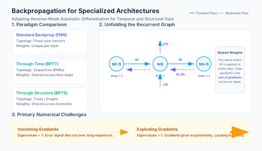
Backpropagation Through Time (BPTT) is the standard algorithm for training Recurrent Neural Networks (RNNs). Unlike feedforward networks where each layer has its own set of weights, an RNN applies the same weight matrix $W$ at every time step.

1. What it is

BPTT is a technique where the recurrent network is "unfolded" into a deep feedforward network where each layer represents a time step. Because the weights are shared across all time steps, the gradient of the loss with respect to a weight matrix is the sum of the gradients at each time step.

2. Why it matters

RNNs are designed to handle sequential data (speech, text, sensor logs). Without BPTT, we could not compute how a weight update at time $t=0$ affects the loss at time $t=100$. It allows the model to "remember" information by propagating error signals back through the hidden states across the temporal dimension.

3. How it works: The Derivation

Consider a simple RNN with hidden state $h_t$ and input $x_t$: $h_t = \sigma(W_h h_{t-1} + W_x x_t + b)$ $y_t = \text{softmax}(W_y h_t + b_y)$

The total loss $\mathcal{L}$ over $T$ time steps is: $\mathcal{L} = \sum_{t=1}^T \mathcal{L}_t$

To compute the gradient with respect to the recurrent weights $W_h$, we apply the chain rule: $\frac{\partial \mathcal{L}}{\partial W_h} = \sum_{t=1}^T \frac{\partial \mathcal{L}_t}{\partial W_h}$

For a specific time step $t$, the gradient depends on all previous states because $h_t$ is a function of $h_{t-1}$, which is a function of $h_{t-2}$, and so on. $\frac{\partial \mathcal{L}t}{\partial W_h} = \sum{k=1}^t \frac{\partial \mathcal{L}t}{\partial y_t} \frac{\partial y_t}{\partial h_t} \left( \prod{j=k+1}^t \frac{\partial h_j}{\partial h_{j-1}} \right) \frac{\partial h_k}{\partial W_h}$

4. Concrete Example: Truncated BPTT Implementation

In practice, unfolding a network for 1,000 steps leads to memory exhaustion and the Vanishing Gradient Problem. We use Truncated BPTT (TBPTT) to limit the backward pass to a fixed number of steps $k$.

import torch
import torch.nn as nn

class SimpleRNN(nn.Module):
    def __init__(self, input_size, hidden_size):
        super(SimpleRNN, self).__init__()
        self.hidden_size = hidden_size
        self.rnn_cell = nn.RNNCell(input_size, hidden_size)
        self.fc = nn.Linear(hidden_size, 1)

    def forward(self, x, h_prev):
        # x: (batch, seq_len, input_size)
        outputs = []
        h_t = h_prev
        for t in range(x.size(1)):
            h_t = self.rnn_cell(x[:, t, :], h_t)
            outputs.append(self.fc(h_t))
        return torch.stack(outputs, dim=1), h_t

# Training Loop with Truncated BPTT
def train_step(model, data, target, h_prev, k_steps=20):
    # Detach hidden state to prevent backprop beyond k_steps
    h_prev = h_prev.detach() 
    
    output, h_final = model(data, h_prev)
    loss = nn.MSELoss()(output, target)
    
    loss.backward() # This performs BPTT for the current window
    optimizer.step()
    optimizer.zero_grad()
    
    return h_final

AI_DEMOI_DEMO### 5. Common Pitfalls: Vanishing and Exploding Gradients The term $\prod_{j=k+1}^t \frac{\partial h_j}{\partial h_{j-1}}$ is the "engine" of BPTT. If the eigenvalues of the weight matrix $W_h$ are less than 1, the gradient shrinks exponentially as it travels back in time (Vanishing Gradient). If they are greater than 1, the gradient grows exponentially (Exploding Gradient).

Problem	Symptom	Solution
Exploding Gradients	Loss becomes NaN, weights overflow	Gradient Clipping (norm scaling)
Vanishing Gradients	Model fails to learn long-term dependencies	LSTM/GRU cells, Identity initialization
Memory Bottleneck	Out of Memory (OOM) on GPU	Truncated BPTT, Gradient Checkpointing

---

Backpropagation Through Structure (BPTS)

While BPTT handles linear sequences, Backpropagation Through Structure (BPTS) generalizes the concept to Recursive Neural Networks (not to be confused with Recurrent). These networks operate on tree-structured data, such as the syntactic parse tree of a sentence or the molecular structure of a chemical compound.

1. What it is

BPTS is an optimization technique for networks where the computational graph is a tree. In a recursive network, a "cell" (similar to an RNN cell) is applied to the children of a node to produce the parent's representation. BPTS propagates the error from the root of the tree down to the leaves.

2. Why it matters

Many real-world phenomena are hierarchical rather than sequential. In Natural Language Processing (NLP), the meaning of a sentence is often better captured by its hierarchical structure (Subject-Verb-Object) than by the linear order of words. BPTS allows the model to learn distributed representations that respect this hierarchy.

3. How it works: The Recursive Step

Let a node $p$ have children $c_1$ and $c_2$. The representation of the parent is: $h_p = \sigma(W [h_{c1}; h_{c2}] + b)$

Where $[h_{c1}; h_{c2}]$ is the concatenation of the children's hidden states. The weight matrix $W$ is shared across all nodes in the tree.

During the backward pass:

1. The gradient is received at node $p$ from its parent.
2. The gradient is also contributed by the local loss function at node $p$ (if applicable).
3. The gradient is backpropagated through the concatenation and the weight matrix $W$ to the children $c_1$ and $c_2$.
4. The gradients for $W$ are accumulated across all nodes in the tree.

4. Concrete Example: Sentiment Analysis on a Parse Tree

Imagine a sentence "Not good" parsed as a tree where "Not" and "good" are leaves.

# Pseudocode for BPTS logic
def backprop_through_structure(node, d_loss_d_hp):
    """
    node: current node in the tree
    d_loss_d_hp: gradient of loss w.r.t. current node's hidden state
    """
    if node.is_leaf():
        # Update leaf embeddings
        node.embedding_grad += d_loss_d_hp
        return

    # 1. Compute local gradient w.r.t. weights W
    # h_p = sigma(W * [h_left, h_right] + b)
    combined_children = concat(node.left.h, node.right.h)
    d_W = outer_product(d_loss_d_hp * sigma_prime, combined_children)
    global_W_grad += d_W

    # 2. Propagate gradient to children
    d_children = W.T @ (d_loss_d_hp * sigma_prime)
    d_left, d_right = split(d_children)

    # 3. Recursive calls
    backprop_through_structure(node.left, d_left)
    backprop_through_structure(node.right, d_right)

5. Variations: Tree-LSTMs

Standard BPTS suffers from the same vanishing gradient issues as RNNs. To solve this, researchers developed the Tree-LSTM, which applies the LSTM gating mechanism to tree structures. In a Tree-LSTM, a parent node has a "forget gate" for each child, allowing it to selectively retain or discard information from specific branches of the hierarchy.

---

Advanced Gradient Management

Training specialized architectures requires more than just the basic algorithm. Several techniques are essential to ensure convergence.

Gradient Clipping

To prevent exploding gradients in BPTT, we scale the gradient if its norm exceeds a threshold $\tau$: $\text{if } |\nabla \mathcal{L}| > \tau: \nabla \mathcal{L} \leftarrow \tau \frac{\nabla \mathcal{L}}{|\nabla \mathcal{L}|}$

Gradient Checkpointing

For extremely long sequences or massive trees, storing all intermediate activations for the backward pass is impossible. Gradient Checkpointing trades computation for memory by only storing activations for a subset of nodes (checkpoints) and re-computing the intermediate activations during the backward pass.

Complexity Analysis

Algorithm	Time Complexity (Forward)	Time Complexity (Backward)	Space Complexity
Standard Backprop	$O(N)$	$O(N)$	$O(N)$
BPTT	$O(T \times H^2)$	$O(T \times H^2)$	$O(T \times H)$
Truncated BPTT	$O(T \times H^2)$	$O(k \times H^2)$	$O(k \times H)$
BPTS	$O(N \times H^2)$	$O(N \times H^2)$	$O(\text{depth} \times H)$

(Where $N$ is nodes/layers, $T$ is time steps, $H$ is hidden size, and $k$ is truncation window.)

---

Backpropagation in Graph Neural Networks (GNNs)

Modern specialized architectures often involve graphs that are neither linear nor tree-like. GNNs use a form of backpropagation that operates on Message Passing phases.

In a GNN, the "forward pass" involves nodes aggregating features from their neighbors. The "backward pass" must propagate gradients through these aggregations. If the graph is static, this is equivalent to backpropagation through a very large, sparse computational graph. If the graph is dynamic or contains cycles, techniques similar to BPTT (iterative message passing) are used, often requiring the system to reach a fixed point or using a fixed number of iterations.

Key Insight: Backpropagation through any specialized architecture is essentially the process of defining a topological sort of the computational graph and applying the chain rule in reverse order. The "specialization" lies in how we handle shared parameters and how we manage the memory of intermediate states.

---

Summary of Best Practices

1. Initialize Carefully: For BPTT, initializing the recurrent weight matrix $W_h$ as an identity matrix or using orthogonal initialization can significantly mitigate vanishing gradients.
2. Monitor Norms: Always track the $L_2$ norm of your gradients. Sudden spikes are a precursor to divergence.
3. Use Frameworks: While understanding the derivation is crucial, use autograd engines (PyTorch, JAX, TensorFlow). They handle the complex bookkeeping of shared weights and structural unfolding more efficiently than manual implementations.
4. Batching: Batching tree structures (BPTS) is significantly harder than batching sequences (BPTT). Use libraries like DGL (Deep Graph Library) or PyTorch Geometric which implement specialized batching kernels for non-linear structures.

AI_STUDY_GUIDEI_STUDY_GUIDE### Flashcards (Conceptual)

• Q: What is the main difference between Backpropagation and BPTT?
  • A: Standard backpropagation assumes independent weights per layer, while BPTT handles shared weights across time steps by summing gradients across the temporal unfolding.
• Q: Why is Truncated BPTT used?
  • A: To reduce memory consumption and prevent the vanishing gradient problem from becoming unmanageable over very long sequences.
• Q: In BPTS, how are weight updates calculated?
  • A: The gradient is calculated at each node in the tree structure, and because the weights are shared across all nodes, the individual gradients are summed to produce the final update.
• Q: What is the "Jacobian" in the context of BPTT?
  • A: It is the matrix of partial derivatives of the hidden state at time $t$ with respect to the hidden state at time $t-1$. Its eigenvalues determine gradient stability.

Quiz: Backpropagation Mastery

1. True/False: In BPTT, the number of layers in the unfolded network is equal to the number of time steps in the input sequence.
2. Multiple Choice: Which technique is specifically designed to handle the "Exploding Gradient" problem?
   • A) Dropout
   • B) Gradient Clipping
   • C) Batch Normalization
   • D) Xavier Initialization
3. Short Answer: Explain why recursive neural networks (BPTS) are more computationally expensive to batch than recurrent neural networks (BPTT).
4. Calculation: If an RNN has a sequence length of 3, and the gradient of the loss w.r.t the hidden state at each step is $\delta_1, \delta_2, \delta_3$, write the simplified expression for the total gradient w.r.t the shared weight $W$.

Study Guide: Specialized Backpropagation

• Core Concept: Backpropagation is Reverse-Mode AD.
• BPTT Focus: Temporal unfolding, weight sharing across time, vanishing/exploding gradients, TBPTT.
• BPTS Focus: Structural unfolding (trees), recursive application of weights, hierarchical representations.
• Implementation: Use detach() for truncation, use sum() for shared weight gradients, use clip_grad_norm_ for stability.
• Further Reading: Rumelhart et al. (1986) for the original backprop; Hochreiter (1991) for vanishing gradients; Goller & Küchler (1996) for BPTS.

Advanced Optimization and Efficiency

In the landscape of machine learning, the transition from theoretical models to production-ready systems is governed by the efficiency of optimization. While the fundamental goal remains the minimization of a loss function $L(\theta)$, the path to that minimum is fraught with computational bottlenecks, vanishing signals, and memory constraints. Advanced optimization focuses on two fronts: the algorithmic efficiency of gradient computation across diverse architectures and the convergence speed provided by higher-order mathematical approximations.

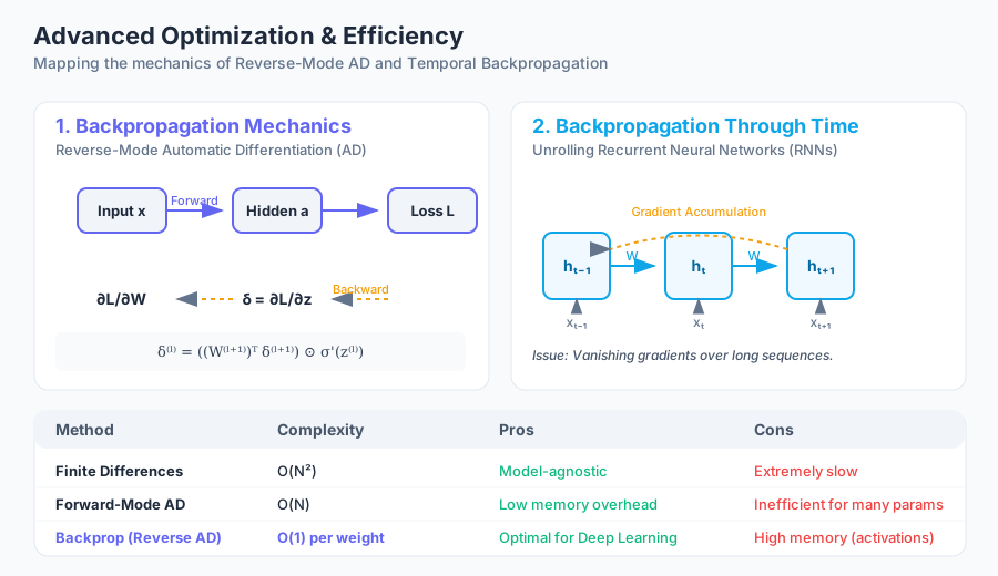
AI_SVGI_SVG## The Foundation: Backpropagation as Reverse-Mode AD

At its core, Backpropagation is an application of the chain rule from calculus, optimized through Dynamic Programming. While often conflated with the entire training process, it is strictly a method for calculating the gradient of a loss function with respect to the weights of a neural network.

1. What it is

Backpropagation is a specific case of Reverse-Mode Automatic Differentiation (AD). It computes the partial derivatives $\frac{\partial L}{\partial w_{ij}}$ by traversing the computational graph from the output back to the input.

Definition: Backpropagation is an efficient algorithm for computing the gradient of a scalar-valued function of multiple variables, specifically designed for functions represented as a directed acyclic graph (DAG) of elementary operations.

2. Why it matters

Before backpropagation became widely recognized in the mid-1980s (notably by Rumelhart, Hinton, and Williams), training deep networks was considered computationally intractable. A naive approach would require $O(N)$ forward passes to compute gradients for $N$ parameters via finite differences. Backpropagation reduces this to a single backward pass, making the complexity $O(1)$ relative to the forward pass cost per parameter.

3. How it works: The Mechanics

The algorithm operates in two distinct phases:

1. Forward Pass: Input data is propagated through the network. At each node, the intermediate activations $a^{(l)}$ and pre-activations $z^{(l)}$ are stored.
2. Backward Pass: The "error" signal $\delta^{(l)}$ is computed starting from the output layer.

Mathematically, for a layer $l$: $$z^{(l)} = W^{(l)}a^{(l-1)} + b^{(l)}$$ $$a^{(l)} = \sigma(z^{(l)})$$

The gradient for the weights is: $$\frac{\partial L}{\partial W^{(l)}} = \delta^{(l)} (a^{(l-1)})^T$$ Where the error $\delta$ is propagated backward: $$\delta^{(l)} = ((W^{(l+1)})^T \delta^{(l+1)}) \odot \sigma'(z^{(l)})$$

4. Comparison of Computational Approaches

Method	Complexity	Pros	Cons
Finite Differences	$O(N^2)$	Simple to implement, model-agnostic	Extremely slow for large $N$
Forward-Mode AD	$O(N)$	Low memory overhead	Inefficient for many parameters, one output
Backpropagation (Reverse-Mode)	$O(1)$ per weight	Highly efficient for many parameters	High memory (must store all activations)

5. Implementation Example (Python/NumPy)

import numpy as np

def sigmoid(x):
    return 1 / (1 + np.exp(-x))

def sigmoid_derivative(x):
    return x * (1 - x)

def backprop_step(x, y, weights_input_hidden, weights_hidden_output):
    # 1. Forward Pass
    hidden_layer_input = np.dot(x, weights_input_hidden)
    hidden_layer_output = sigmoid(hidden_layer_input)
    
    output_layer_input = np.dot(hidden_layer_output, weights_hidden_output)
    predicted_output = sigmoid(output_layer_input)
    
    # 2. Compute Output Error
    error = y - predicted_output
    d_predicted_output = error * sigmoid_derivative(predicted_output)
    
    # 3. Backpropagate to Hidden Layer
    error_hidden_layer = d_predicted_output.dot(weights_hidden_output.T)
    d_hidden_layer = error_hidden_layer * sigmoid_derivative(hidden_layer_output)
    
    # 4. Gradient Calculation
    grad_weights_hidden_output = hidden_layer_output.T.dot(d_predicted_output)
    grad_weights_input_hidden = x.T.dot(d_hidden_layer)
    
    return grad_weights_input_hidden, grad_weights_hidden_output

---

Temporal Dynamics: Backpropagation Through Time (BPTT)

When dealing with sequential data, standard backpropagation fails because the network's state at time $t$ depends on its state at $t-1$. Backpropagation Through Time (BPTT) solves this by "unfolding" the recurrent neural network (RNN).

1. What it is

BPTT is the application of the backpropagation algorithm to a Recurrent Neural Network that has been unrolled into a deep feedforward network where each layer represents a time step and all layers share the same parameters.

2. Why it matters

RNNs are essential for time-series, speech, and natural language. However, the shared weight matrix $W$ is applied repeatedly. This creates a deep dependency chain, leading to the Vanishing/Exploding Gradient Problem, where the gradient signal either disappears or grows exponentially as it travels back through many time steps.

3. Mechanics of Unfolding

Consider a hidden state $h_t = \sigma(W_h h_{t-1} + W_x x_t)$. To compute the gradient of the loss $L$ at time $T$ with respect to $W_h$: $$\frac{\partial L_T}{\partial W_h} = \sum_{t=1}^T \frac{\partial L_T}{\partial h_T} \frac{\partial h_T}{\partial h_t} \frac{\partial h_t}{\partial W_h}$$

The term $\frac{\partial h_T}{\partial h_t}$ involves a product of Jacobian matrices: $$\frac{\partial h_T}{\partial h_t} = \prod_{k=t+1}^T \frac{\partial h_k}{\partial h_{k-1}}$$

4. Variations of BPTT

Variation	Description	Use Case
Full BPTT	Unfolds the network for the entire sequence length.	Short sequences, high precision.
Truncated BPTT	Unfolds for a fixed number of steps $k$, then stops.	Long sequences (e.g., character-level language models).
Real-Time Recurrent Learning (RTRL)	Computes gradients forward in time.	Online learning where sequences are infinite.

5. Common Pitfalls: The Vanishing Gradient

In BPTT, if the eigenvalues of the weight matrix $W_h$ are less than 1, the product $\prod \frac{\partial h_k}{\partial h_{k-1}}$ will shrink to zero.

• Symptom: The model fails to learn long-term dependencies (e.g., the beginning of a sentence doesn't affect the end).
• Solution: Use Gated architectures (LSTM, GRU) or Gradient Clipping.

AI_DEMOI_DEMO--

Structural Generalization: Backpropagation Through Structure (BPTS)

While BPTT handles linear sequences, Backpropagation Through Structure (BPTS) extends the concept to recursive structures, such as trees or graphs.

1. What it is

BPTS is a gradient-based technique for training Recursive Neural Networks. Unlike Recurrent networks (linear), Recursive networks process data in a hierarchical fashion (e.g., a parse tree of a sentence).

2. Why it matters

In Natural Language Processing, sentences have a nested, hierarchical structure. BPTS allows the model to learn distributed representations of phrases and sentences by following the syntax tree, rather than just the word order.

3. How it works

1. Topology: The network structure is defined by the input (e.g., a binary tree).
2. Forward Pass: Nodes are computed from leaves to root.
3. Backward Pass: Gradients are propagated from the root down to the leaves. If a weight $W$ is used at multiple nodes in the tree, the total gradient is the sum of gradients at each node.

4. Comparison: BPTT vs. BPTS

Feature	BPTT (Recurrent)	BPTS (Recursive)
Data Structure	Linear Sequence	Tree / DAG
Dependency	Temporal (Time $t$)	Structural (Parent/Child)
Complexity	$O(T)$ where $T$ is length	$O(N)$ where $N$ is number of nodes
Primary Application	Speech, Sensors	NLP Parsing, Chemistry (Molecules)

---

Second-Order Optimization: The Levenberg–Marquardt (LM) Algorithm

Standard backpropagation uses first-order derivatives (the gradient). However, first-order methods can be slow to converge near local minima. Second-order methods use the Hessian matrix (second derivatives) to find the optimal step size and direction.

1. What it is

The Levenberg–Marquardt (LM) algorithm is an optimization technique that interpolates between the Gauss-Newton algorithm and the method of Gradient Descent. It is specifically designed for least-squares problems.

2. Why it matters

LM is significantly faster than standard gradient descent for small-to-medium-sized neural networks. It avoids the "zig-zagging" behavior of first-order methods in narrow valleys of the loss surface.

3. Mechanics and the Quasi-Hessian

The update rule for LM is: $$\theta_{k+1} = \theta_k - [J^T J + \mu I]^{-1} J^T e$$

Where:

• $J$ is the Jacobian matrix containing first derivatives of the errors with respect to parameters.
• $J^T J$ is the Quasi-Hessian approximation.
• $e$ is the vector of network errors.
• $\mu$ is the damping factor.

Key Insight: When $\mu$ is large, the algorithm behaves like Gradient Descent with a small step size. When $\mu$ is small (or zero), it behaves like the Gauss-Newton method, which has quadratic convergence properties.

4. Comparison of Optimization Methods

Method	Update Rule	Convergence Speed	Memory Cost
Gradient Descent	$-\alpha \nabla L$	Linear	Low ($O(N)$)
Newton's Method	$-H^{-1} \nabla L$	Quadratic	Very High ($O(N^2)$)
Levenberg-Marquardt	$-(J^T J + \mu I)^{-1} J^T e$	Super-linear	High ($O(N^2)$)

5. Memory Efficiency in LM

The primary bottleneck of LM is storing the Jacobian $J$ and inverting the matrix $J^T J$. For a network with $N$ parameters and $M$ training patterns, $J$ is an $M \times N$ matrix. Modern implementations use Jacobian-free products or Memory-Efficient LM which calculates $J^T J$ and $J^T e$ incrementally: $$J^T J = \sum_{i=1}^M j_i j_i^T$$ This allows the algorithm to run without ever storing the full Jacobian matrix in memory.

---

Synthesis: Choosing the Right Optimizer

Efficiency in deep learning is not a "one size fits all" solution. The choice of algorithm depends on the architecture and the scale of the data.

1. For Massive Scale (LLMs, Vision Transformers): First-order methods with momentum (Adam, AdamW) are preferred. The $O(N^2)$ memory cost of second-order methods like LM is prohibitive when $N$ is in the billions.
2. For High Precision (Control Systems, Shallow Networks): LM is superior. It converges in far fewer iterations and can find much more precise minima.
3. For Structured Data (Code, Syntax): BPTS is necessary to capture the recursive nature of the input, even if it is more complex to implement than BPTT.

Summary of Efficiency Trade-offs

Scenario	Recommended Approach	Reason
Real-time streaming data	Truncated BPTT	Limits memory usage and latency.
Small dataset, high accuracy needed	Levenberg-Marquardt	Faster convergence to global/local minima.
Standard Deep Learning	Backprop + Adam	Best balance of speed and memory.
Hierarchical/Nested data	BPTS	Captures structural dependencies.

AI_STUDY_GUIDEI_STUDY_GUIDE## Study Guide: Advanced Optimization and Efficiency

Core Concepts to Master

1. Reverse-Mode AD: Understand why backpropagation is a dynamic programming problem. Be able to derive the gradient for a single neuron.
2. The Unfolding Process: Visualize how an RNN becomes a deep feedforward network. Understand that $W$ is the same at every layer.
3. Vanishing Gradients: Explain why the product of many small numbers leads to zero and how this kills learning in BPTT.
4. The Jacobian vs. The Hessian: Know that the Jacobian is first-order (slopes) and the Hessian is second-order (curvature).
5. Damping Factor ($\mu$): Explain how $\mu$ in the LM algorithm switches the strategy between Gradient Descent and Gauss-Newton.

Mathematical Identities to Remember

• Chain Rule: $\frac{dz}{dx} = \frac{dz}{dy} \cdot \frac{dy}{dx}$
• LM Update: $\Delta \theta = (J^T J + \mu I)^{-1} J^T e$
• RNN State: $h_t = f(Wh_{t-1} + Ux_t)$

Practical Application Tips

• When using BPTT, always monitor the norm of the gradients. If they exceed a threshold, use Gradient Clipping.
• If your model is not converging with SGD, try a second-order approximation like L-BFGS or LM if the parameter count allows.
• For BPTS, ensure your input data is pre-processed into a consistent tree structure (e.g., using a Penn Treebank parser).