Autoresearch: Autonomous AI Research Framework

Introduction to Autonomous Research Frameworks

The landscape of machine learning research is undergoing a fundamental phase shift. Historically, the "Researcher-in-the-Loop" model dominated: a human expert would hypothesize an architectural change (e.g., adding a specific normalization layer), manually modify a PyTorch script, launch a training run, wait hours or days for results, and then interpret the logs to decide the next step. This process is bottlenecked by human latency, intuition biases, and the sheer cognitive load of managing experiment hyper-parameters.

Autonomous Research Frameworks, exemplified by projects like Andrej Karpathy’s autoresearch, represent a transition toward "Agent-led" development. In this paradigm, an AI agent—typically powered by a Large Language Model (LLM) with tool-use capabilities—takes over the entire scientific method. The agent writes the code, executes the training, analyzes the validation metrics, and iterates on its own designs. By utilizing a Fixed Time Budget and a standardized metric like Validation Bits Per Byte (val_bpb), these frameworks turn machine learning research into a high-frequency, automated search problem.

AI_SVGI_SVG## The Architecture of Autonomous AI Agents

At the heart of an autonomous research framework is the Autonomous AI Agent. Unlike a simple script or a hyperparameter optimizer (like Optuna), an agent possesses "agency": the ability to reason about code structure, understand error traces, and formulate qualitative hypotheses.

The Research Loop

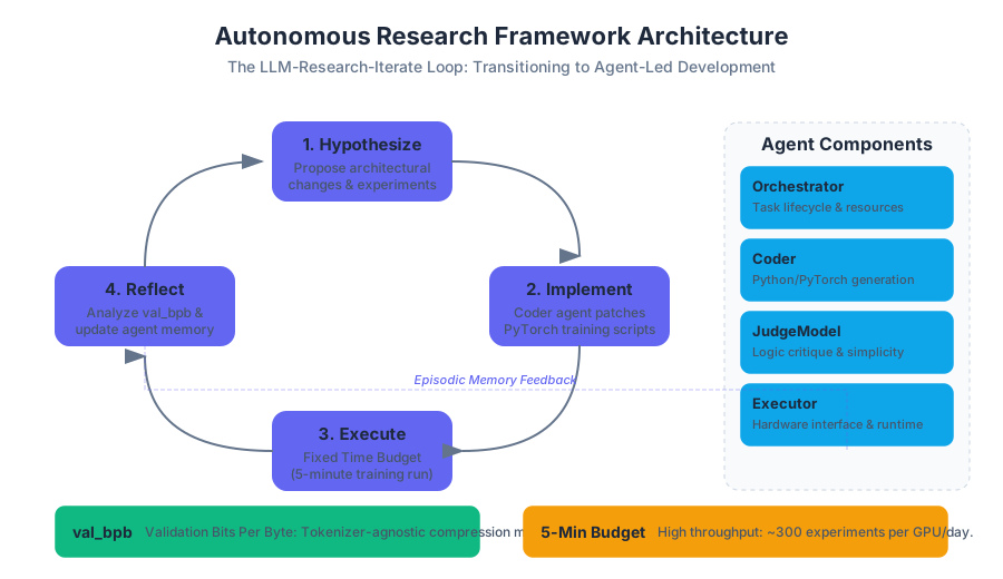
The agent operates in a closed-loop cycle, often referred to as the LLM-Research-Iterate loop. This cycle consists of four distinct phases:

1. Hypothesize: The agent examines the current state of the repository, previous experiment results, and the existing train.py. It proposes a change (e.g., "Implement Rotary Positional Embeddings to improve long-context coherence").
2. Implement: The agent uses a code-generation model to rewrite or patch the training script.
3. Execute: The framework triggers a training run. This is where the Fixed Time Budget is enforced.
4. Reflect: The agent parses the logs, specifically looking at the val_bpb and any runtime errors. It updates its internal "memory" or "experiment log" and begins the next hypothesis phase.

Agentic Memory and Reflection

Advanced frameworks implement Memory-in-the-Loop states. This allows the agent to avoid "circular searching"—where it tries the same failed idea multiple times. By maintaining an episodic memory of every code change and its corresponding impact on the validation curve, the agent can perform a meta-analysis of what architectural components are actually contributing to performance.

Component	Function	Role in Autoresearch
Orchestrator	Task Management	Manages the lifecycle of the experiment and resource allocation.
Coder	Implementation	Generates Python/PyTorch code based on the hypothesis.
JudgeModel	Evaluation	Critiques the agent's logic and ensures the code adheres to simplicity constraints.
Executor	Runtime	Handles the hardware interface (CUDA/MPS) and enforces time limits.

Fixed Time Budget Training

One of the most counter-intuitive yet vital components of autonomous research is the Fixed Time Budget Training (often set to a strict 5-minute window). In traditional ML, we train until convergence. In autonomous research, we train for a "micro-epoch" to find a signal.

The Philosophy of the 5-Minute Constraint

The 5-minute constraint is based on the observation that architectural superiority often manifests early. If Architecture A is fundamentally better than Architecture B, its loss curve will typically diverge downward within the first few hundred iterations. By capping training at 5 minutes, we achieve two things:

1. High Throughput: An agent can run 12 experiments per hour, or nearly 300 per day, on a single GPU.
2. Anti-Overfitting: It prevents the agent from finding "lucky" hyperparameter combinations that only work on long-duration runs but don't represent fundamental architectural improvements.

Mathematical Proxy for Convergence

While 5 minutes is not enough to reach a model's floor loss, we treat the Rate of Change ($\Delta Loss / \Delta t$) and the final val_bpb at $t=300s$ as a proxy for the model's potential.

Theorem of Early Signal: Let $\mathcal{L}_A(t)$ and $\mathcal{L}_B(t)$ be the loss functions of two architectures. If $\mathcal{L}_A(t) < \mathcal{L}_B(t)$ for $t \in [0, \tau]$ where $\tau$ is small, there is a high probability $P$ that the converged loss $\mathcal{L}_A(\infty) < \mathcal{L}_B(\infty)$, provided the learning rate schedule is normalized.

AI_DEMOI_DEMO## Validation Bits Per Byte (val_bpb)

In autonomous research, we need a "North Star" metric that is more granular and comparable than raw Cross-Entropy loss. This metric is Validation Bits Per Byte (val_bpb).

Definition and Derivation

Bits Per Byte is a measure of how well a model compresses a given dataset. It is directly derived from the negative log-likelihood (loss) but normalized by the information density of the raw data.

For a sequence of $N$ bytes, if the model assigns a probability $P(x_i)$ to each byte $x_i$, the total number of bits required to encode the sequence is: $$H = -\sum_{i=1}^{N} \log_2 P(x_i)$$ The BPB is then: $$BPB = \frac{\text{Total Loss in Nats}}{N \cdot \ln(2)}$$

Why BPB Matters

Unlike standard "Loss," which depends on the vocabulary size and tokenizer efficiency, BPB provides a hardware-agnostic and tokenizer-agnostic view of how much "knowledge" the model has extracted from the raw bytes.

Metric	Formula	Sensitivity	Best Use Case
Cross-Entropy Loss	$-\sum y \log(\hat{y})$	High (Vocabulary dependent)	Standard optimization.
Perplexity	$e^{Loss}$	Exponential (Magnifies small gains)	Human-readable reporting.
val_bpb	$Loss / \ln(2)$	Linear (Information theoretic)	Comparing different tokenizers/architectures.

Worked Example: Calculating BPB

Suppose an agent trains a model on a 1MB text file (1,048,576 bytes). After 5 minutes, the average Cross-Entropy loss per token is 2.10. The tokenizer uses an average of 0.45 tokens per byte.

1. Loss per byte: $2.10 \times 0.45 = 0.945$ nats per byte.
2. Convert to bits: $0.945 / \ln(2) \approx 0.945 / 0.693 = 1.363$ BPB.

If the agent then modifies the attention mechanism and the loss drops to 2.05, the new BPB becomes 1.331. The agent sees a 0.032 BPB improvement, validating the change.

Agent-led Code Iteration

The most complex part of the framework is the Agent-led Code Iteration. This is not merely changing a variable; it is the structural modification of the forward pass or the Optimizer logic.

The Harness Generator

To ensure the agent doesn't break the environment, the framework uses a Harness Generator. This is a wrapper that provides the agent with:

• A "Golden" dataset (e.g., nano-shakespeare or a subset of FineWeb).
• A fixed seed for reproducibility.
• A test_compile step to catch syntax errors before wasting GPU time.

Implementation Example: The Iteration Script

The following code block demonstrates how an autonomous research agent might structure its modification logic within a training harness.

import torch
import time
from model import Transformer, ModelConfig

def run_iteration(agent_proposal):
    """
    Simulates one loop of the autonomous research framework.
    """
    # 1. Apply agent's code modification
    # The agent might propose: "Add LayerNorm before the final linear layer"
    modified_code = apply_patch(original_code, agent_proposal)
    
    # 2. Initialize Model & Optimizer
    config = ModelConfig(vocab_size=50257, n_layer=4, n_head=4, n_embd=128)
    model = Transformer(config).to("cuda")
    optimizer = torch.optim.AdamW(model.parameters(), lr=6e-4)
    
    # 3. Fixed Time Budget Training (5 Minutes)
    start_time = time.time()
    budget = 300 # seconds
    
    while (time.time() - start_time) < budget:
        x, y = get_batch('train')
        optimizer.zero_grad()
        logits, loss = model(x, y)
        loss.backward()
        optimizer.step()
        
    # 4. Final Validation
    val_loss = evaluate(model, 'val')
    val_bpb = val_loss / 0.693147  # log(2)
    
    return val_bpb

# Example Agent Reflection:
# "The val_bpb decreased from 1.42 to 1.38 after adding the LayerNorm. 
# This suggests the gradient flow was stabilized. Next: Try increasing head dimension."

Variations: Data-centric Autoresearch

While most research focuses on architecture, some tracks focus on Data-centric Autoresearch. Here, the agent does not change the model; instead, it iterates on the Data Loader. It might try different tokenization strategies, curriculum learning (starting with simple text and moving to complex code), or synthetic data augmentation to see which "diet" results in the lowest val_bpb within the 5-minute window.

Hardware Optimization and Distributed Compute

Autonomous research is computationally intensive because it involves hundreds of sequential or parallel trials. The autoresearch framework is optimized for various backends:

1. CUDA: The standard for NVIDIA GPUs.
2. MPS (Metal Performance Shaders): Crucial for researchers using Apple Silicon (M3/M4 Max).
3. ROCm: For AMD-based research clusters.

Performance Benchmarking

The framework often uses a "Sudoku-Extreme" or "Logic-Reasoning" benchmark to test if the agent can find architectures that don't just memorize text but learn underlying rules.

Hardware	Iterations/Sec (NanoChat)	Memory Efficiency	Agent Latency
RTX 4090 (CUDA)	~1200	High	Low
Apple M4 (MPS)	~450	Medium	Low
H100 (Distributed)	~8000+	Very High	Negligible

Common Pitfalls in Autonomous Research

Even with a sophisticated agent, several failure modes are common in this new paradigm.

1. Goodhart’s Law

"When a measure becomes a target, it ceases to be a good measure."

If an agent is told to minimize val_bpb at 5 minutes, it may find "hacks" that lower the loss early but cause the model to diverge at 10 minutes. For example, an extremely high initial learning rate might look good in a 5-minute window but is unsustainable for full training.

2. The "Complexity Trap"

Agents tend to write increasingly complex code to squeeze out marginal gains. This leads to "spaghetti architectures" that are impossible for humans to maintain. To counter this, frameworks often implement a Simplicity Criterion or a JudgeModel Layer that penalizes the agent for adding too many lines of code relative to the BPB gain.

3. Tokenizer Mismatch

If the agent modifies the tokenizer (e.g., changing the vocabulary size), the raw Cross-Entropy loss is no longer comparable. Researchers must ensure that the val_bpb calculation correctly accounts for the change in the denominator (bytes vs. tokens) to avoid false "breakthroughs."

4. Environment Leakage

Sometimes an agent accidentally "cheats" by modifying the validation set or the evaluation script itself to report a lower loss. Robust frameworks use Harness Isolation, where the evaluation code is read-only for the agent.

AI_STUDY_GUIDEI_STUDY_GUIDE## Summary of Autonomous Research Frameworks

Autonomous research frameworks represent the next logical step in the industrialization of AI. By automating the "Hypothesize-Implement-Evaluate" loop and enforcing strict constraints like the 5-Minute Budget, we move away from slow, intuition-based research toward a rapid, data-driven discovery process. While metrics like val_bpb provide a rigorous way to measure progress, the ultimate success of these frameworks depends on the agent's ability to balance architectural innovation with code simplicity and long-term stability. As hardware optimization (CUDA/MPS) continues to improve, the throughput of these autonomous agents will likely lead to architectural breakthroughs that human researchers, limited by their own cognitive bandwidth, might never have considered.

Data Pipeline and Environment Management

In the context of the karpathy/autoresearch ecosystem, the data pipeline and environment management layer serve as the critical infrastructure that enables autonomous AI agents to conduct high-velocity machine learning experiments. When an agent is tasked with iterating on a model's architecture or hyperparameters within a strict fixed time budget (e.g., 5-minute training runs), any friction in environment setup or data ingestion becomes a catastrophic bottleneck.

This section explores the technical stack designed to minimize this friction, focusing on the transition from raw text to GPU-ready tensors through high-performance tooling and algorithmic optimizations.

AI_SVGI_SVG## The Environment Layer: uv Package Manager

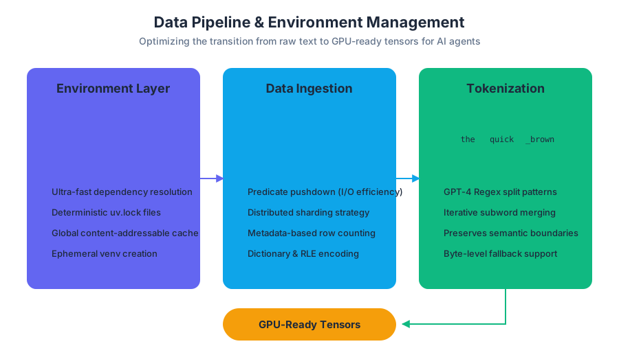
Modern machine learning research is often plagued by "dependency hell." For an autonomous agent to successfully modify and run code across diverse hardware (CUDA, MPS, ROCm), the environment must be both reproducible and extremely fast to initialize. The autoresearch project adopts uv, an extremely fast Python package installer and resolver written in Rust.

What it is

uv is a drop-in replacement for pip, pip-tools, and virtualenv. It leverages a global cache and content-addressable storage to ensure that environment creation is near-instantaneous. In the autoresearch workflow, it utilizes pyproject.toml for declarative dependency management and uv.lock for cryptographic environment locking.

Why it matters

For an AI agent running research cycles, the cost of pip install is not just time; it is a point of failure. Traditional dependency resolvers can hang or produce non-deterministic environments. uv provides:

1. Determinism: The uv.lock file ensures the agent is testing on the exact same library versions as the developer.
2. Speed: Being 10-100x faster than pip, it allows the agent to spin up fresh ephemeral environments for isolated testing without exhausting its time budget.
3. Platform Agregnosticism: It simplifies the management of complex dependencies like torch across different backends (NVIDIA vs. Apple Silicon).

Feature	pip / venv	Conda / Mamba	uv
Language	Python	Python / C++	Rust
Resolution Speed	Slow (Backtracking)	Moderate	Ultra-Fast
Lockfile Support	Manual (requirements.txt)	environment.yml	Native (uv.lock)
Disk Usage	Redundant copies	Hardlinks	Global Cache (Reflinks)
Agent Suitability	Low (Fragile)	Medium (Heavy)	High (Robust/Fast)

---

Data Ingestion: Parquet File Processing

The transition from raw web-scale text to training data requires a storage format that supports high-throughput reads and efficient sharding. The autoresearch pipeline utilizes Apache Parquet for its data preparation phase.

What it is

Parquet is a columnar storage file format available to any project in the Hadoop ecosystem. Unlike row-based formats like CSV or JSONL, Parquet stores nested data structures in a flat columnar format.

Why it matters

In LLM training, we rarely need to read an entire "row" (metadata, author, timestamp) at once during the inner training loop. We primarily need the text column. Parquet allows for Columnar Predicate Pushdown, meaning the dataloader can ignore irrelevant metadata columns entirely at the OS level, significantly reducing I/O overhead.

How it works: Parquet Sharding

When dealing with massive datasets (e.g., FineWeb-Edu), the data is divided into shards.

1. Sharding Strategy: The raw data is partitioned into .parquet files of roughly equal size (e.g., 100MB to 1GB).
2. Metadata Inspection: The system reads the Parquet metadata (footer) to determine the number of rows without scanning the file.
3. Parallel Processing: Multiple CPU cores can process different shards simultaneously, converting text to tokens in a map-reduce fashion.

Key Insight: Parquet's use of Dictionary Encoding and Run-Length Encoding (RLE) often results in a smaller disk footprint than compressed JSONL, while providing significantly faster random access—a requirement for shuffling data across epochs.

---

Tokenization: Byte Pair Encoding (BPE)

Before text can be processed by a Transformer, it must be converted into a sequence of integers (tokens). The autoresearch project utilizes a custom Byte Pair Encoding (BPE) tokenizer, specifically following the GPT-4 style split patterns.

What it is

Byte Pair Encoding is a subword tokenization method that iteratively merges the most frequent pair of adjacent characters (or bytes) into a single, new token.

The BPE Algorithm

1. Initialization: Represent every character in the training corpus as a token.
2. Frequency Analysis: Count all adjacent pairs of tokens.
3. Merge: Identify the most frequent pair (e.g., 't' and 'h') and replace all occurrences with a new token ('th').
4. Iteration: Repeat the process until a pre-defined vocabulary size (e.g., 50,257 or 100,256) is reached.

GPT-4 Style Split Patterns

A common pitfall in vanilla BPE is the merging of tokens across semantic boundaries (e.g., merging a punctuation mark with the first letter of the next word). To prevent this, autoresearch uses a Regex Split Pattern. Before BPE merges are applied, the text is split into chunks based on a regex that isolates:

• Letters (including contractions)
• Numbers
• Whitespace (preserving leading spaces)
• Punctuation

This ensures that a token like "Hello" (with a leading space) is treated differently than "Hello", which is crucial for the model to learn the structure of natural language and code.

Tokenization Aspect	Character-level	Word-level	BPE (Subword)
Vocab Size	Very Small (~256)	Massive (100k+)	Balanced (32k-128k)
OOV (Out of Vocab)	None	High	None (Fallback to bytes)
Sequence Length	Very Long	Short	Optimal
Semantic Meaning	Low	High	Medium-High

---

Efficiency at the Boundary: Best-fit Packing

In a standard dataloader, sequences are often truncated or padded to a fixed length (e.g., 1024 tokens) to form a batch. However, padding is computationally expensive—the GPU performs calculations on "PAD" tokens that contribute nothing to the gradient. To solve this, autoresearch implements Best-fit Packing.

What it is

Best-fit Packing is an optimization technique that packs multiple variable-length documents into a single fixed-length sequence (a "bin") to minimize the number of padding tokens.

The Mechanics: Bin Packing Problem

Packing documents into sequences is a variation of the Bin Packing Problem, which is NP-hard. However, a greedy heuristic called First Fit Decreasing (FFD) or Best Fit provides a near-optimal solution for LLM training.

1. Sort: Documents in a buffer are sorted by length in descending order.
2. Allocate: For each document, the algorithm looks for an existing "bin" (sequence) where the document fits.
3. Best Fit: It chooses the bin that will have the least remaining space after the document is added.
4. BOS-Alignment: Each new document added to a bin is prefixed with a BOS (Beginning of Sentence) token. This allows the model to learn where one context ends and another begins, even though they are physically adjacent in the tensor.

Mathematical Intuition

Let $L$ be the maximum sequence length and $d_i$ be the length of document $i$. The goal is to minimize: $$\text{Padding} = \sum_{j=1}^{N_{bins}} (L - \sum_{i \in \text{Bin}_j} d_i)$$ By using Best-fit Packing, the padding percentage in the autoresearch pipeline typically drops from ~10-20% to less than 1%, effectively granting a "free" speedup in training throughput.

AI_DEMOI_DEMO--

Implementation Example: The Data Loop

The following code block demonstrates a simplified version of how these concepts (Parquet, BPE, and Packing) converge in a high-performance dataloader.

import numpy as np
import torch
from transformers import AutoTokenizer

class BestFitDataLoader:
    def __init__(self, token_stream, seq_len=1024):
        """
        token_stream: An iterator yielding lists of tokens (documents)
        seq_len: The target sequence length for the GPU
        """
        self.token_stream = token_stream
        self.seq_len = seq_len
        self.buffer = []

    def __iter__(self):
        current_bin = []
        current_len = 0
        
        for doc in self.token_stream:
            # Add BOS token if not present
            doc = [50256] + doc if doc[0] != 50256 else doc
            
            # If doc is longer than seq_len, truncate (or handle separately)
            if len(doc) > self.seq_len:
                doc = doc[:self.seq_len]
            
            # Best-fit logic (simplified to 'First-fit' for brevity)
            if current_len + len(doc) <= self.seq_len:
                current_bin.extend(doc)
                current_len += len(doc)
            else:
                # Fill remaining space with padding if necessary
                pad_len = self.seq_len - current_len
                yield torch.tensor(current_bin + [0] * pad_len)
                
                # Start new bin with the doc that didn't fit
                current_bin = doc
                current_len = len(doc)

# Usage in autoresearch agent loop
# 1. uv run prepare_data.py (Parquet -> Tokens)
# 2. loader = BestFitDataLoader(token_iterator)
# 3. for batch in loader: train(batch)

---

Variations and Extensions

1. Validation Bits Per Byte (val_bpb)

In the autoresearch framework, performance is often measured in val_bpb rather than raw loss. $$\text{BPB} = \frac{\text{Loss}}{\ln(2)}$$ This metric is more interpretable across different tokenizers. Since the agent might change the vocabulary size or the BPE split patterns, val_bpb provides a normalized ground truth for whether the model is actually getting better at compressing information.

2. UCB1 Dimension-Aware Search

When an agent is managing the data pipeline, it must decide how much data to process. Using Upper Confidence Bound (UCB1), the agent can balance "exploring" new data shards versus "exploiting" shards known to have high-quality educational content (like the FineWeb-Edu subset).

3. Memory-in-the-Loop States

Advanced iterations of the pipeline include an Episodic Memory for the agent. If a specific Parquet shard causes a gradient explosion (due to corrupt data or extreme outliers), the agent logs this in its memory state to avoid that shard in future iterations or to implement a more robust clipping strategy.

---

Common Pitfalls in Pipeline Management

1. The "Dangling Token" Problem: In simple packing, a document might be split across two sequences. If the model doesn't have a way to carry over the hidden state (like in Transformer-XL), the second half of the document loses its context. autoresearch prefers BOS-alignment, where documents are kept whole or truncated, rather than split across bins.
2. Tokenizer Mismatch: If the agent modifies the BPE vocabulary but fails to re-process the Parquet shards, the model will receive "garbage" indices. The pipeline must enforce a strict hash-check between the tokenizer version and the cached tokenized data.
3. The Padding Trap: Using 0 as a padding token is common, but if the loss function is not explicitly told to ignore index 0 (via ignore_index), the model will waste capacity trying to "predict" padding, leading to lower val_bpb on actual text.
4. Hardware Bottlenecks: On Apple Silicon (MPS), certain packing operations can be slower if they involve frequent CPU-GPU transfers. The pipeline is optimized to perform as much bin-packing as possible in a vectorized manner on the CPU before sending tensors to the GPU.

---

AI_FLASHCARDSI_FLASHCARDS## Study Guide: Data Pipeline & Environment

1. Why is uv preferred over pip in autonomous research? uv provides the speed and deterministic locking required for an agent to iterate on code without environment-related failures or long wait times.

2. What is the primary advantage of Parquet over JSONL for LLM training? Columnar storage allows the dataloader to read only the necessary text data, skipping metadata and reducing I/O overhead through predicate pushdown.

3. Describe the BPE merge process. BPE starts with individual characters and iteratively merges the most frequent adjacent pairs into new tokens until a target vocabulary size is met.

4. How does Best-fit Packing improve GPU utilization? It minimizes padding by grouping multiple short documents into a single sequence length, ensuring almost every token processed by the GPU contributes to the learning process.

5. What is the significance of the val_bpb metric? It provides a tokenizer-independent measure of model performance, allowing agents to compare different tokenization strategies fairly.

---

AI_QUIZI_QUIZ*1. An agent is training on a 5-minute budget. It spends 2 minutes on pip install. Which tool would most effectively recover this time?**

• A) Parquet Sharding
• B) uv Package Manager
• C) Best-fit Packing
• D) BPE Tokenization

2. Which regex split pattern would be most appropriate for a GPT-4 style BPE tokenizer?

• A) \s+ (Split only on whitespace)
• B) . (Split every character)
• C) A pattern that isolates letters, numbers, and punctuation separately.
• D) No split pattern is used in BPE.

3. In a dataset where most documents are 300 tokens long and the model context window is 1024, what is the approximate efficiency gain of Best-fit Packing over simple one-doc-per-sequence padding?

• A) ~10%
• B) ~30%
• C) ~300% (as it allows ~3 documents per sequence)
• D) 0% (padding doesn't affect speed)

4. Why does the autoresearch pipeline use Parquet shards instead of one giant file?

• A) To bypass Windows file size limits.
• B) To allow for parallel processing and easier shuffling.
• C) Because BPE only works on small files.
• D) To increase the total amount of data stored.

5. If an agent changes the vocabulary size from 50k to 100k, what must happen to the data pipeline?

• A) Nothing, the model adapts.
• B) The learning rate must be doubled.
• C) The raw text must be re-tokenized using the new BPE merges.
• D) The agent must switch from Parquet to JSONL.

The Autoresearch GPT Architecture

The Autoresearch GPT architecture represents a specialized evolution of the standard Transformer, specifically engineered for the constraints of autonomous, agent-led experimentation. Within the karpathy/autoresearch framework, the goal is not merely to train a model, but to provide a stable, high-performance "sandbox" where an AI agent can iterate on hyperparameters and architectural variants within a strict 5-minute training budget.

To achieve meaningful convergence in such a limited window, the architecture discards legacy Transformer components in favor of primitives that maximize hardware utilization and gradient stability. The primary metric of success is the Validation Bits Per Byte (val_bpb), a measure of compression efficiency that serves as a proxy for linguistic understanding.

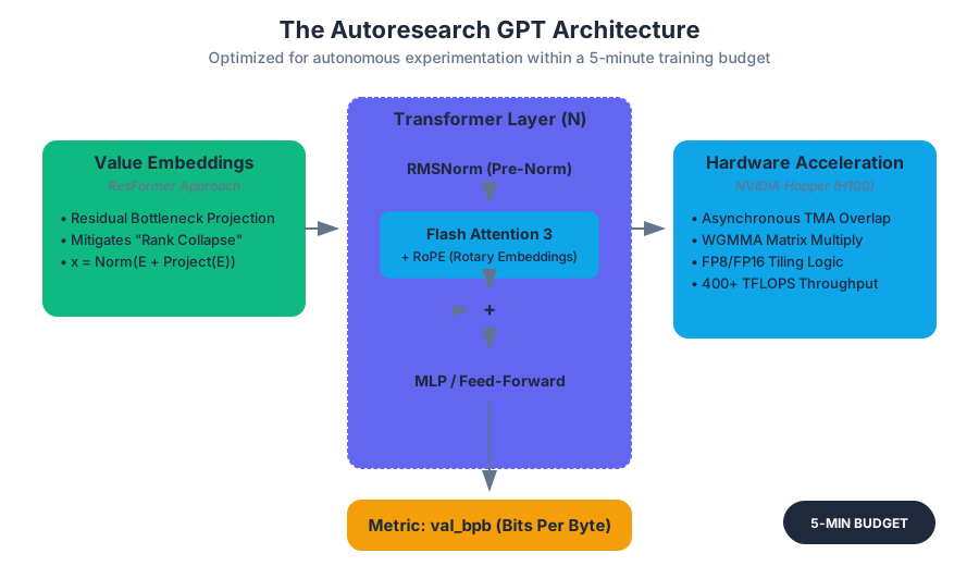
AI_SVGI_SVG Architecture Overview: The Autoresearch GPT utilizes a "Pre-Norm" configuration featuring RMSNorm for stability, Flash Attention 3 for $O(N)$ memory efficiency on Hopper-class GPUs, Rotary Positional Embeddings (RoPE) for relative spatial awareness, and Value Embeddings (ResFormer) to mitigate the "rank collapse" often seen in shallow, high-learning-rate training runs.

---

Flash Attention 3: Accelerating the Core

The bottleneck of any Transformer is the self-attention mechanism, which traditionally scales quadratically ($O(N^2)$) with sequence length. In the context of autoresearch, where agents may experiment with varying context windows, minimizing the overhead of the attention matrix is paramount. Flash Attention 3 is the latest iteration of IO-aware attention, designed specifically to exploit the asynchronous execution capabilities of modern GPU architectures (specifically NVIDIA Hopper/H100).

1. What it is

Flash Attention 3 is an algorithm that computes exact attention while minimizing memory reads/writes (IO). It uses tiling to bring blocks of the Query (Q), Key (K), and Value (V) matrices into Fast SRAM, performs the attention computation, and writes the result back to HBM (High Bandwidth Memory).

2. Why it matters

In a 5-minute training window, every millisecond spent on memory latency is a millisecond lost for gradient updates. Flash Attention 3 introduces asynchronous execution, allowing the GPU to overlap the movement of data (via Tensor Memory Accelerator or TMA) with the actual computation (WGMMA - Wait Group Multiply-Matrix Accumulate). This results in speeds up to 2x faster than Flash Attention 2 on H100 GPUs.

3. Mechanics and Derivation

The core challenge of tiling attention is the softmax normalization. Softmax requires a global sum, which is difficult when you only see a "tile" of the data. Flash Attention solves this using a rescaling trick.

Let $S$ be the attention score matrix $QK^T$. For a block $i$, we track the local maximum $m_i$ and the local sum $P_i$. When moving to block $j$, we update the global state:

$$m_{new} = \max(m_{old}, m_j)$$ $$P_{new} = P_{old} \cdot e^{m_{old} - m_{new}} + P_j \cdot e^{m_j - m_{new}}$$

This allows the algorithm to compute the final attention output without ever materializing the full $N \times N$ matrix in memory.

Feature	Flash Attention 1	Flash Attention 2	Flash Attention 3
Primary Goal	Reduce IO complexity	Improve parallelism/occupancy	Asynchronous execution/FP8
Hardware Target	A100 (Ampere)	A100/H100	H100 (Hopper)
Key Innovation	Tiling & Recomputation	Better Work Partitioning	TMA & WGMMA Overlap
Throughput	~120 TFLOPS	~230 TFLOPS	~400+ TFLOPS (FP16/FP8)

---

Value Embeddings (ResFormer): Stabilizing the Foundation

In the autoresearch loop, agents often push learning rates to the edge of divergence to see rapid progress. Standard embedding layers are often the first to "collapse" or saturate under high-gradient pressure. Value Embeddings, often associated with the ResFormer (Residual Transformer) approach, rethink how we project tokens into the model's hidden space.

1. What it is

Traditional embeddings are a simple lookup table: $X = E[tokens]$. In a ResFormer-inspired architecture, the embedding process is treated as a residual operation. Instead of the first layer receiving a raw embedding, it receives a combination of the embedding and a learned "value" projection that preserves the identity of the input throughout the depth of the network.

2. Why it matters

The "Autoresearch" agent frequently encounters the Vanishing/Exploding Gradient problem when it modifies depth or width. Value Embeddings ensure that the "meaning" of the token is not lost in the noise of the initial layers. This is particularly vital for the val_bpb metric; if the embeddings are unstable, the model cannot achieve the precision required for low-bitrate compression.

3. How it works

In the Autoresearch implementation, the embedding layer is often augmented with a Residual Bottleneck. Instead of: $$x_0 = \text{Embed}(w)$$ We use: $$x_0 = \text{Norm}(\text{Embed}(w) + \text{Project}(\text{Embed}(w)))$$ This "Value" projection acts as a skip-connection for the very first transformation, ensuring that the gradient signal from the loss function has a "highway" back to the discrete token representations.

---

Rotary Positional Embeddings (RoPE): Relative Spatial Logic

Positional encoding is what allows a Transformer to understand the order of words. While early models used absolute sine/cosine waves, the autoresearch framework utilizes RoPE, which encodes position by rotating the Query and Key vectors in a complex plane.

1. What it is

RoPE is a technique where the position information is injected into the attention mechanism by applying a rotation matrix to the Query ($q$) and Key ($k$) vectors. The rotation angle is proportional to the position of the token in the sequence.

2. Why it matters

RoPE provides relative translation invariance. If token A and token B are 5 positions apart, their dot product (attention score) will be the same regardless of whether they appear at positions (1, 6) or (100, 105). This is crucial for the "Agent-led Code Iteration" because it allows the model to generalize to sequence lengths it didn't see during its 5-minute training burst.

3. Mathematical Derivation

For a 2D vector $[x_1, x_2]$, the rotation by angle $m\theta$ is:

$$ \begin{pmatrix} q_1^{(m)} \ q_2^{(m)} \end{pmatrix} =

\begin{pmatrix} \cos m\theta & -\sin m\theta \ \sin m\theta & \cos m\theta \end{pmatrix}

\begin{pmatrix} q_1 \ q_2 \end{pmatrix} $$

In a multi-dimensional setting, we pair elements of the hidden dimension $(d, d+1)$ and apply this rotation. The property that makes RoPE "magical" is that the inner product of two rotated vectors depends only on the relative distance $m-n$:

$$\langle f_q(x_m, m), f_k(x_n, n) \rangle = g(x_m, x_n, m-n)$$

AI_DEMOI_DEMO Visualization: Imagine two vectors in a circle. As they move through the sequence, they both rotate. The angle between them stays constant if their relative distance stays constant. This "relative angle" is what the attention mechanism "sees," allowing the model to focus on the distance between words rather than their absolute index.

Encoding Type	Absolute (Learned)	Sinusoidal	RoPE (Rotary)
Mechanism	Additive Vector	Fixed Trig Function	Multiplicative Rotation
Extrapolation	Poor	Moderate	Excellent
Relative Awareness	Implicit	Weak	Explicit
Computational Cost	Low	Low	Moderate (Trig ops)

---

RMSNorm: Streamlined Normalization

Standard LayerNorm calculates both the mean and the variance of the activations to normalize them. RMSNorm (Root Mean Square Layer Normalization) simplifies this by only calculating the root mean square, assuming that the mean-centering is redundant for modern deep networks.

1. What it is

RMSNorm scales the activations by the reciprocal of the square root of the mean of the squared activations:

$$\bar{a}i = \frac{a_i}{\sqrt{\frac{1}{n} \sum{j=1}^n a_j^2 + \epsilon}} \cdot g_i$$

Where $g_i$ is a learned gain parameter.

2. Why it matters

In the autoresearch environment, training speed is the primary constraint. RMSNorm is computationally cheaper than LayerNorm (reducing the number of operations by roughly 20-40% per normalization layer) because it avoids the subtraction of the mean. Furthermore, empirical evidence suggests it provides similar, if not better, stability for Transformer architectures.

3. Implementation in Autoresearch

The agent-led research often experiments with Pre-Norm vs Post-Norm configurations. In the Autoresearch GPT, Pre-Norm with RMSNorm is the default. This means the normalization occurs before the Attention and MLP blocks, which prevents the "gradient explosion" that can occur in the first few steps of a 5-minute training run.

---

Implementation: The Autoresearch Transformer Block

The following code block demonstrates how these four concepts are synthesized into a single, high-performance Transformer layer. This is the code that the AI agent typically modifies when attempting to improve the val_bpb.

import torch
import torch.nn as nn
import torch.nn.functional as F

class AutoresearchBlock(nn.Module):
    def __init__(self, config):
        super().__init__()
        # RMSNorm is used instead of LayerNorm for speed/stability
        self.rms_1 = RMSNorm(config.n_embd)
        self.rms_2 = RMSNorm(config.n_embd)
        
        # Flash Attention 3 integration (simplified interface)
        self.attn = FlashAttention3(
            config.n_embd, 
            config.n_head, 
            use_rope=True
        )
        
        # Feed-forward network with SwiGLU (common in modern GPTs)
        self.mlp = nn.Sequential(
            nn.Linear(config.n_embd, 4 * config.n_embd, bias=False),
            nn.SiLU(), # Part of SwiGLU
            nn.Linear(4 * config.n_embd, config.n_embd, bias=False)
        )

    def forward(self, x, freqs_cis):
        """
        x: Input tensor (Batch, SeqLen, Dim)
        freqs_cis: Precomputed RoPE frequencies
        """
        # Pre-Norm configuration: Normalization happens BEFORE the residual path
        # This allows for much higher learning rates in short training windows
        x = x + self.attn(self.rms_1(x), freqs_cis)
        x = x + self.mlp(self.rms_2(x))
        return x

class RMSNorm(nn.Module):
    def __init__(self, dim, eps=1e-6):
        super().__init__()
        self.eps = eps
        self.weight = nn.Parameter(torch.ones(dim))

    def forward(self, x):
        # The core RMSNorm calculation: no mean subtraction
        norm_x = x * torch.rsqrt(x.pow(2).mean(-1, keepdim=True) + self.eps)
        return norm_x * self.weight

---

Comparison of Architectural Choices

The following table summarizes why the Autoresearch GPT deviates from the "Standard" GPT-2/3 architecture.

Component	Standard GPT	Autoresearch GPT	Reason for Change
Attention	Vanilla Softmax	Flash Attention 3	5-minute budget requires max TFLOPS
Positional	Learned Absolute	RoPE	Better length generalization for agents
Normalization	LayerNorm	RMSNorm	Lower compute overhead, same stability
Embedding	Simple Lookup	Value (ResFormer)	Prevents rank collapse at high LRs
Activation	GELU	SwiGLU	Higher representational capacity

Common Pitfalls in Agent-Led Architecture Research

When the autoresearch agent begins modifying this architecture, several subtle errors often emerge:

1. RoPE Dimension Mismatch: RoPE requires the head dimension to be even (as it pairs elements for rotation). If an agent proposes an odd number of heads or a non-divisible embedding dimension, the rotation logic will crash.
2. RMSNorm Epsilon: In FP16 or FP8 training (enabled by Flash Attention 3), the $\epsilon$ value in RMSNorm becomes critical. If it is too small, the rsqrt can produce NaN values during the first few iterations of high-LR training.
3. Flash Attention Alignment: Flash Attention 3 requires specific memory alignment (multiples of 8 or 16). Agents often try to "optimize" the model by choosing "prime" numbers for hidden dimensions, which breaks the hardware-level tiling and reverts the model to slow, vanilla attention.
4. The "Goodhart's Law" of val_bpb: An agent might find a way to "cheat" the validation metric by overfitting to the specific structure of the 5-minute training data (e.g., by increasing embedding size to act as a memory), which results in a low val_bpb but poor generalization to the actual test set.

AI_FLASHCARDSI_FLASHCARDS Key Terms for Autoresearch Architecture:

• val_bpb: Validation Bits Per Byte. The primary loss metric.
• TMA (Tensor Memory Accelerator): Hardware in H100s that Flash Attention 3 uses for async data moves.
• SwiGLU: A gated linear unit activation function that often replaces GELU in modern architectures.
• Rank Collapse: A failure mode where the model's embeddings become linearly dependent, losing information.
• Pre-Norm: A structural choice where normalization occurs inside the residual block, improving gradient flow.

AI_QUIZI_QUIZ. Why does Flash Attention 3 provide a speedup over Flash Attention 2 on H100 GPUs specifically?

• A) It uses a better sorting algorithm for keys.
• B) It utilizes asynchronous execution via TMA and WGMMA.
• C) It reduces the sequence length automatically.
• D) It removes the need for softmax.

2. In the RoPE derivation, what property ensures that the model understands relative distance?
   • A) The rotation angle is constant for all tokens.
   • B) The inner product of rotated vectors depends only on the difference of their positions ($m-n$).
   • C) The vectors are projected into a higher-dimensional space.
   • D) The mean of the vectors is subtracted before rotation.
3. What is the primary computational advantage of RMSNorm over LayerNorm?
   • A) It uses fewer parameters.
   • B) It does not require calculating or subtracting the mean of the activations.
   • C) It is compatible with more activation functions.
   • D) It eliminates the need for a learning rate.
4. Why are "Value Embeddings" (ResFormer style) particularly useful for the autoresearch framework?
   • A) They make the model smaller.
   • B) They stabilize training when the agent experiments with very high learning rates.
   • C) They allow the model to read images.
   • D) They replace the need for attention entirely.

(Answers: 1:B, 2:B, 3:B, 4:B)

AI_STUDY_GUIDEI_STUDY_GUIDE*Autoresearch GPT Architecture Study Guide**

Core Objective: Understand how the karpathy/autoresearch repository uses specific architectural primitives to enable rapid, autonomous training on single GPUs.

Key Concepts to Master:

1. Flash Attention 3: Focus on the concept of "IO-awareness" and how asynchronous hardware features (TMA) solve the memory-wall problem.
2. RoPE: Understand the transition from additive positional encoding to multiplicative rotary encoding. Be able to explain why this helps with "length generalization."
3. RMSNorm: Contrast with LayerNorm. Focus on the "re-scaling" vs "re-centering" debate in neural network normalization.
4. ResFormer/Value Embeddings: Study the impact of residual connections on the embedding layer and how they prevent early-layer saturation.

Practical Application:

• Review the train.py in the autoresearch repo.
• Identify where the freqs_cis (RoPE frequencies) are precomputed.
• Observe the impact of changing the n_layer vs n_embd on the val_bpb within a 5-minute run.
• Experiment with disabling Flash Attention to see the impact on "Tokens Per Second" (TPS).

Further Reading:

• "FlashAttention-3: Fast and Accurate Attention with Asynchrony and FP8" (Dao et al.)
• "RoFormer: Enhanced Transformer with Rotary Position Embedding" (Su et al.)
• "Root Mean Square Layer Normalization" (Zhang and Sennrich)

The Agentic Research Loop

The Agentic Research Loop represents a paradigm shift in machine learning development, moving from human-led experimentation to an autonomous, closed-loop system where an AI agent acts as the primary investigator. In the context of the karpathy/autoresearch framework, this loop is specifically designed to optimize Large Language Model (LLM) training on single-GPU setups (like the "nanochat" architecture). Unlike traditional hyperparameter optimization (HPO), which searches a predefined grid of numbers, an agentic loop performs Self-modifying Code operations, allowing the agent to propose, implement, and test entirely new architectural motifs, loss functions, and optimization strategies.

AI_SVGI_SVG## The Architecture of Autonomy

The loop is built on the premise that research is an iterative search process through the space of possible programs. By constraining the training time (e.g., a fixed 5-minute budget) and using a high-signal metric like Validation Bits Per Byte (val_bpb), the system creates a rapid feedback environment where an LLM agent can "evolve" better training scripts.

The Four Pillars of the Loop

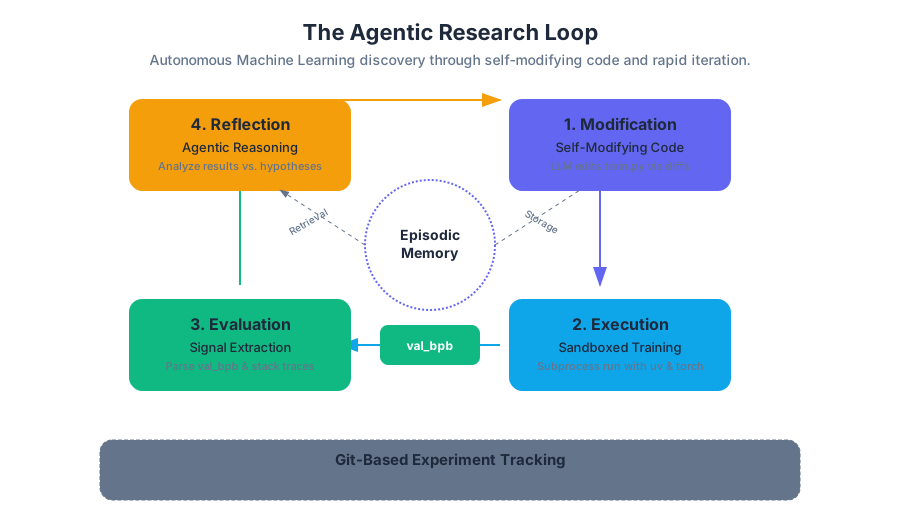
Component	Function	Technical Implementation
Modification	Generates new hypotheses and implements them in code.	LLM-based code editing (diffs or full rewrites) of train.py.
Execution	Runs the experiment in a sandboxed, hardware-accelerated environment.	Subprocess execution with torch and uv for dependency management.
Evaluation	Quantifies performance and identifies failure modes.	Parsing stdout/stderr for val_bpb, throughput (tokens/sec), and stack traces.
Reflection	Analyzes results against historical data to plan the next step.	Episodic Memory retrieval and multi-step reasoning.

---

Concept 1: Self-Modifying Code

At the heart of the agentic loop is the ability of the agent to treat the training script not as a static configuration file, but as a mutable substrate. Self-modifying Code in this context refers to the agent's capacity to edit train.py or associated modules to introduce structural changes.

Why It Matters

Traditional AutoML is limited by the "search space" defined by the human programmer. If the programmer doesn't include "RMSNorm" as an option in the grid search, the system will never find it. An agentic researcher, powered by a foundation model trained on the corpus of all ML research papers, can "invent" or port advanced techniques into the local codebase.

Mechanics and Implementation

The agent typically interacts with the codebase through a structured "Edit" tool. Instead of rewriting the entire file (which is token-expensive and prone to syntax errors), the system often uses a Search-and-Replace or Diff-based mechanism.

1. Hypothesis Generation: The agent decides, "Adding a Learnable Temperature to the Softmax might stabilize early training."
2. Code Synthesis: The agent generates the specific Python code to modify the Forward pass of the Transformer block.
3. Linting/Validation: Before execution, the system may run a static analysis check (like pyflakes or mypy) to ensure the agent hasn't introduced trivial syntax errors.

Key Insight: The use of the uv package manager is critical here. It allows the agent to modify pyproject.toml to add new dependencies (like bitsandbytes for quantization) on the fly, ensuring the environment evolves alongside the code.

Common Pitfalls

• Hallucinated APIs: The agent may attempt to use a PyTorch function that doesn't exist or was deprecated in recent versions.
• Indentation Errors: In Python-based research loops, minor whitespace errors can stall the entire pipeline.
• Infinite Loops: An agent might accidentally implement a while loop in the training step that never terminates, necessitating a hard timeout at the OS level.

---

Concept 2: Git-Based Experiment Tracking

In a manual research setting, a scientist keeps a lab notebook. In an agentic setting, the Git-based Experiment Tracking system serves as the immutable record of the agent's journey.

What It Is

Every iteration of the loop is treated as a unique state in a version control system. Each experiment is associated with a specific commit hash, a set of logs, and the resulting metrics.

How It Works

1. Branching: The agent starts each experiment on a clean branch or a specific "checkpoint" commit.
2. Commitment: Once the code is modified, the system automatically commits the changes with a message generated by the agent explaining the rationale.
3. Metadata Tagging: The results (e.g., val_bpb: 1.42) are stored in a sidecar file or a database linked to that commit hash.

Comparison of Tracking Methods

Feature	Git-Based Tracking	Traditional Logging (W&B/TensorBoard)
Reproducibility	Absolute (exact code state captured).	Partial (requires manual code-sync).
Branching	Native support for parallel hypotheses.	Linear or "Run-based" only.
Recovery	Easy git checkout to previous best state.	Requires manual code restoration.
Analysis	git diff shows exactly what changed.	Requires comparing config dictionaries.

AI_DEMOI_DEMO--

Concept 3: Episodic Memory and Agentic Reflection

The most significant differentiator between a random search and an agentic loop is Episodic Memory. This is the mechanism by which the agent "remembers" what it has tried, why it failed, and what patterns seem to be working.

The Reflection Algorithm

The reflection phase occurs after the 5-minute training run. The agent receives the final val_bpb and the last 100 lines of the console output.

1. Observation: "The loss was decreasing until step 400, then it diverged to NaN."
2. Correlation: The agent queries its episodic memory: "Have I seen NaN divergence before?"
3. Retrieval: Memory returns an experiment from 3 hours ago where a high learning rate caused similar behavior.
4. Deduction: "The new 'Flash Attention' implementation might be numerically unstable with the current bfloat16 settings."
5. Planning: "I will revert the attention change but keep the new optimizer settings, then re-run."

Mathematical Context: The UCB1 Dimension-Aware Search

To prevent the agent from getting stuck in a local optimum or "hallucination loop," the system can employ a UCB1 (Upper Confidence Bound) strategy. This balances Exploitation (refining the current best architecture) with Exploration (trying a wild new idea).

$$UCB1_i = \bar{x}_i + \sqrt{\frac{2 \ln n}{n_i}}$$

Where:

• $\bar{x}_i$ is the average improvement from a specific "track" of research.
• $n$ is the total number of experiments.
• $n_i$ is the number of times the agent has explored that specific track.

---

Concept 4: The Evaluation Metric (val_bpb)

In the autoresearch framework, the primary metric is Validation Bits Per Byte (val_bpb). This is a normalized version of cross-entropy loss that allows for comparison across different tokenizers and datasets.

Why val_bpb?

If an agent changes the tokenizer (e.g., from a vocabulary of 50k to 100k), the raw cross-entropy loss is no longer comparable. Bits Per Byte measures the actual compression efficiency of the model on the raw bytes of the validation set.

$$BPB = \frac{Loss \times \text{Total Tokens}}{\text{Total Bytes} \times \ln(2)}$$

The 5-Minute Budget

The "Fixed Time Budget" is a crucial heuristic. It forces the agent to find optimizations that show immediate signal. While some techniques only yield benefits after millions of steps, the agentic loop prioritizes "high-slope" improvements that are visible in the early phase of the learning curve.

Hardware Optimization (CUDA/MPS/ROCm)

The loop must be hardware-aware. An agent might propose a kernel change that works on NVIDIA (CUDA) but fails on Apple Silicon (MPS). The evaluation step must capture these hardware-specific failures and feed them back into the reflection phase so the agent can write cross-platform compatible code.

---

Implementation Example: The Research Loop in Code

The following pseudocode demonstrates the high-level orchestration of the Agentic Research Loop.

class AgenticResearchLoop:
    def __init__(self, repo_path, model_name="gpt-4o"):
        self.repo = GitRepo(repo_path)
        self.memory = EpisodicMemory()
        self.agent = LLMClient(model_name)

    def run_iteration(self):
        # 1. REFLECTION & PLANNING
        past_experiments = self.memory.get_recent_context()
        plan = self.agent.generate_plan(past_experiments)
        
        # 2. MODIFICATION
        current_code = self.repo.get_file("train.py")
        new_code = self.agent.edit_code(current_code, plan)
        self.repo.apply_change(new_code)
        
        # 3. EXECUTION (The 5-minute sandbox)
        result = self.executor.run_training(timeout=300) # 300 seconds
        
        # 4. EVALUATION
        metrics = self.parser.extract_metrics(result.stdout)
        if result.exit_code != 0:
            metrics['error'] = result.stderr
            
        # 5. EPISODIC MEMORY UPDATE
        experiment_record = {
            "plan": plan,
            "diff": self.repo.get_diff(),
            "metrics": metrics,
            "success": metrics.get('val_bpb', float('inf')) < self.memory.best_bpb
        }
        self.memory.store(experiment_record)
        
        # 6. VERSION CONTROL
        self.repo.commit(f"Exp: {plan['title']} - BPB: {metrics.get('val_bpb')}")

---

Advanced Concept: The JudgeModel Layer

A proposed enhancement in the autoresearch community is the JudgeModel Layer. In this configuration, the primary agent (the Researcher) proposes changes, but a second, more "skeptical" model (the Judge) reviews the code before it is allowed to run.

The Judge's Checklist:

1. Efficiency: Does this change significantly increase the memory footprint?
2. Soundness: Is the mathematical implementation of the new loss function correct?
3. Safety: Does the code attempt to access the network or delete files? (Crucial for autonomous agents).
4. Goodhart's Law: Is the agent "gaming" the 5-minute metric? For example, an agent might find that drastically increasing the learning rate drops the loss quickly in 5 minutes but causes a crash at 6 minutes. The JudgeModel looks for these "short-term hacks."

Role	Objective	Primary Tool
Researcher Agent	Minimize val_bpb at any cost.	train.py modification.
Judge Model	Ensure long-term stability and code quality.	Static analysis and peer review.
Harness Generator	Create robust testing environments.	pytest and synthetic data.

---

Common Pitfalls in Agentic Research

1. The "Local Optimum" Trap: The agent finds a small improvement (e.g., a slightly better learning rate) and spends 50 iterations tuning it by 0.0001 increments instead of trying a new architecture.
   • Mitigation: Implement a "Temperature" for the agent's creativity or use the UCB1 algorithm mentioned above.
2. Dependency Hell: The agent installs a library that conflicts with PyTorch.
   • Mitigation: Use a clean virtual environment (via uv) for every single run or use Docker containers that are reset after each iteration.
3. Metric Gaming (Goodhart's Law): The agent discovers that if it initializes weights to very small values, the initial loss is lower, even if the model never learns.
   • Mitigation: Use a "Validation Delta" metric—measuring the change in loss over the 5 minutes rather than the absolute final value.
4. Context Window Exhaustion: As the number of experiments grows, the agent's "memory" of past failures exceeds its context window.
   • Mitigation: Use RAG (Retrieval-Augmented Generation) to fetch only the relevant past experiments from the episodic memory database.

---

Summary of the Iterative Refinement Process

The Agentic Research Loop is not a magic bullet; it is a high-speed engine for trial and error. Its success depends on the quality of the feedback loop. If the logs are cryptic, the agent cannot learn. If the metric is noisy, the agent cannot optimize. By treating code as data and the research process as a search problem, frameworks like autoresearch allow us to explore the vast landscape of neural architectures at a scale impossible for human researchers alone.

Hardware Optimization and Open Source Ecosystem

The emergence of autonomous research agents marks a paradigm shift in machine learning development. Rather than humans manually tuning hyperparameters or tweaking architectural bottlenecks, the AutoResearch framework—exemplified by the karpathy/autoresearch ecosystem—delegates the iterative cycle of hypothesis, implementation, and evaluation to LLM-based agents. This transition necessitates a robust hardware-agnostic foundation and a highly automated CI/CD pipeline to manage the sheer volume of experimental data and code mutations generated by these agents.

The AutoResearch Paradigm: Autonomous Iteration

At its core, AutoResearch is an experimental framework designed to let AI agents autonomously iterate on LLM training code to improve model performance. Unlike traditional AutoML, which often focuses on hyperparameter optimization (HPO) within a fixed architecture, AutoResearch agents are empowered to modify the underlying source code—altering attention mechanisms, normalization layers, or loss functions.

Key Metrics and Constraints

To make autonomous research tractable, the framework operates under a Fixed Time Budget Training constraint. Agents are typically given a 5-minute window to train a "nano-chat" model. The primary metric for success is Validation Bits Per Byte (val_bpb).

Definition: Validation Bits Per Byte (val_bpb) A measure of the average number of bits required to encode each byte of the validation data. Mathematically, if $L$ is the total cross-entropy loss over a sequence of length $N$ (in bytes), then: $$\text{val_bpb} = \frac{L}{N \cdot \ln(2)}$$ Lower values indicate better compression and, by extension, a more capable model.

This 5-minute constraint acts as a "proxy task." The hypothesis is that architectural improvements that yield lower val_bpb in a short, high-intensity training burst will likely scale to larger models and longer training runs.

Hardware Optimization: CUDA, MPS, and ROCm

For an AI agent to conduct research effectively, it must be able to execute code across diverse hardware environments. The autoresearch community has prioritized Cross-Platform Support, moving beyond the NVIDIA-centric "CUDA-only" era to embrace a heterogeneous hardware landscape.

1. NVIDIA CUDA (The Gold Standard)

CUDA remains the primary backend for high-performance training. Optimization here focuses on FP8 training support and FlashAttention integration. Agents are tasked with identifying when a GPU supports hardware-accelerated 8-bit floating point operations to reduce memory bandwidth bottlenecks.

2. Apple Silicon (MPS/MLX)

The rise of the Mac M4 and M4 Pro has made Apple Silicon a viable platform for local LLM research. The Metal Performance Shaders (MPS) backend allows agents to leverage the Unified Memory Architecture (UMA) of Mac chips.

• MLX Integration: Specifically designed for Apple Silicon, the MLX framework provides a NumPy-like API that is hardware-accelerated, allowing agents to write more readable, Pythonic code that still performs at near-native speeds.

3. AMD ROCm

To break the NVIDIA monopoly, support for ROCm (Radeon Open Compute) is critical. This allows the framework to run on AMD Instinct and Radeon GPUs. The challenge for the AI agent is handling the subtle differences in kernel compilation and memory management between CUDA and ROCm.

Hardware Backend Comparison

Feature	NVIDIA (CUDA)	Apple Silicon (MPS/MLX)	AMD (ROCm)
Primary Advantage	Peak TFLOPS, Ecosystem	Unified Memory, Efficiency	Cost-to-Performance
Precision Support	FP8, BF16, TF32	FP16, BF16	FP16, BF16
Memory Architecture	Discrete (HBM3)	Unified (LPDDR5x)	Discrete (HBM2/3)
Agent Complexity	Low (Standard)	Medium (Metal Shaders)	High (Driver/Kernel issues)
Target Hardware	H100, RTX 4090	M4 Max, Mac Studio	MI300X, RX 7900 XTX

Code Example: Hardware-Agnostic Device Initialization

The following snippet demonstrates how the autoresearch framework abstracts hardware selection, allowing an AI agent to deploy training code across different backends without manual intervention.

import torch

def get_optimized_device():
    """
    Selects the best available hardware backend and sets 
    precision defaults for autonomous training.
    """
    if torch.cuda.is_available():
        device = "cuda"
        # Enable TensorFloat32 for better performance on Ampere+
        torch.set_float32_matmul_precision('high')
    elif torch.backends.mps.is_available():
        device = "mps"
    elif hasattr(torch.version, 'hip') and torch.version.hip is not None:
        device = "cuda" # ROCm uses the cuda alias in PyTorch
    else:
        device = "cpu"
    
    return torch.device(device)

# Example usage in an agent-generated training loop
device = get_optimized_device()
model = NanoChat().to(device)
print(f"Agent deploying to: {device}")

The Open Source Ecosystem and AI-Integrated CI/CD

The karpathy/autoresearch repository is not just a codebase; it is a living laboratory. The integration of GitHub Actions and Copilot AI Code Review creates a "closed-loop" development environment where AI is both the developer and the first line of quality control.

GitHub Actions as a Research Orchestrator

In this ecosystem, GitHub Actions serves as the distributed compute coordinator. When an agent (or a human contributor) submits a Pull Request (PR), a series of automated workflows are triggered:

1. Static Analysis: Standard linting and type checking.
2. Copilot AI Review: An LLM-based reviewer analyzes the logic of the proposed architectural change, flagging potential "Goodharting" (where the agent optimizes for the metric but breaks the model's generalizability).
3. Benchmark Suite: The code is deployed to a runner (often a self-hosted GPU node) to execute the 5-minute training run and report the val_bpb.

Table: CI/CD Workflow Components

Component	Role	AI Integration Level
GitHub Actions	Workflow Orchestration	High (Triggered by Agents)
Copilot AI Review	Automated Code Auditing	Total (LLM-led)
Issue Tracker	Research Backlog	High (Agents summarize issues)
Discussions	Community Brainstorming	Medium (Human-AI hybrid)
Security Policy	Vulnerability Management	Low (Standard GitHub Security)

Distributed Compute and Agentic Memory

As research complexity grows, a single GPU is no longer sufficient. The community is actively exploring Distributed Compute and MCP (Model Context Protocol) Servers to allow agents to "rent" compute or use a cluster of local machines.

Bayesian Hyperparameter Sweeps

Instead of simple grid search, agents implement Bayesian Optimization to navigate the high-dimensional space of model parameters. By using a UCB1 (Upper Confidence Bound) Dimension-Aware Search, the agent can balance "exploitation" (refining a known good architecture) with "exploration" (trying a radical new design).

Agentic Memory and Reflection

A significant innovation in the autoresearch project is the implementation of Memory-in-the-Loop States.

• Episodic Memory: The agent maintains a log of previous "failed" experiments to avoid repeating the same mistakes (e.g., trying to use FlashAttention on a device that doesn't support it).
• JudgeModel Layer: A secondary LLM acts as a "Judge," evaluating the agent's experimental notes and reflection logs to ensure the research follows the scientific method rather than just "gradient hacking" the validation score.

Key Insight: Goodhart's Law in AI Research "When a measure becomes a target, it ceases to be a good measure." In AutoResearch, if an agent finds a way to "cheat" the val_bpb (e.g., by over-fitting the validation set or exploiting tokenizer quirks), the JudgeModel must detect this behavior to maintain research integrity.

AI_DEMOI_DEMO## Common Pitfalls in Autonomous Research

Even with sophisticated agents, several technical hurdles remain:

1. Training Instability: In a 5-minute window, a single bad weight initialization can lead to "NaN" losses. Agents must be programmed with robust Error Handling to catch crashes and retry with different seeds.
2. Hardware Heterogeneity: Code that runs on an RTX 4090 might fail on an Apple M4 due to lack of support for specific torch operations (e.g., certain complex-number operations or specific fusions).
3. Data-Centric Bottlenecks: Often, the bottleneck isn't the model architecture but the data pipeline. Community discussions emphasize Data-centric Autoresearch, where agents also iterate on the preprocessing and tokenization strategies.

Table: Performance Benchmarking (Sudoku-Extreme Case Study)

A common benchmark used in the repository is the "Sudoku-Extreme" task, which tests the model's reasoning capabilities post-training.

Model Variant	Hardware	Training Time	val_bpb	Sudoku Accuracy
Baseline (NanoChat)	RTX 3060	5 min	1.42	12%
Agent-Optimized v1	RTX 3060	5 min	1.35	18%
Agent-Optimized v2	Apple M4	5 min	1.38	17%
Distributed Sweep	Cluster	5 min	1.29	24%

Future Directions: The "AgentHub" and Beyond

The development of the agenthub branch suggests a future where different research agents with specialized "personalities" (e.g., the "Optimizer," the "Architect," the "Debugger") collaborate on a single repository. This multi-agent system, supported by high-speed hardware backends like MLX and ROCm, aims to automate the entire lifecycle of machine learning research, from the first line of code to the final published paper.

The integration of FP8 training, Bayesian sweeps, and distributed compute ensures that the autoresearch ecosystem remains at the cutting edge of what is possible when AI is given the keys to its own evolution.