Applied Linear Algebra and Least Squares
Institution: MIT
1 study materials · 9 sections
This course provides a practical introduction to linear algebra, focusing on the core concepts of vectors, matrices, and least squares methods. It emphasizes real-world applications such as machine learning, control systems, and data fitting while maintaining a streamlined mathematical framework. Students will explore how to represent data, solve systems of linear equations, and optimize models using QR factorization and iterative algorithms.
Course Sections
Vector Fundamentals and Inner Products
Key concepts: Scalar-vector multiplication · Unit vector · Sparse vector · Inner product · Complexity (flops)
Covers basic vector notation, scalar-vector multiplication, addition, and the definition of the inner product.
Vector Fundamentals and Inner Products
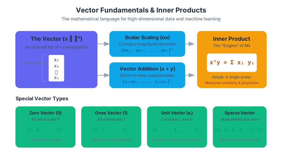
In the landscape of modern computational science, the vector is the fundamental atom of data. Whether representing a point in physical space, a sequence of stock prices over time, or the high-dimensional embedding of a word in a large language model, vectors provide a unified mathematical language for describing the world. This article explores the foundational mechanics of vectors, moving from basic arithmetic to the inner product—the engine that powers nearly all of machine learning and signal processing.
Vector Basics: The Geometry of Data
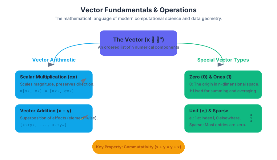
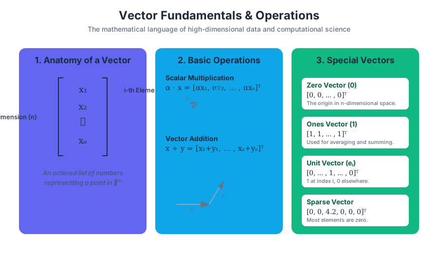
A vector is an ordered list of $n$ numbers, typically written as a column. In the context of applied linear algebra, we denote a vector $x$ as belonging to the set $\mathbb{R}^n$, where $n$ is the dimension or size of the vector. The individual numbers within the vector, $x_1, x_2, \dots, x_n$, are referred to as its entries, components, or elements.
What it is
Mathematically, a vector $x$ is defined as: $$x = \begin{bmatrix} x_1 \ x_2 \ \vdots \ x_n \end{bmatrix}$$ While we often visualize vectors as arrows in 2D or 3D space, in high-dimensional applications (where $n$ might be millions), we treat them as abstract points in an $n$-dimensional manifold.
Why it matters
Vectors allow us to group related quantities into a single mathematical object. This "chunking" of data enables us to perform operations on entire datasets simultaneously rather than iterating through individual numbers. In engineering, a vector might represent the state of a system (position, velocity, acceleration); in economics, it might represent a portfolio of assets.
Common Vector Notations and Types
| Term | Notation | Description |
|---|---|---|
| Dimension | $n$ | The number of elements in the vector. |
| $i$-th element | $x_i$ | The scalar value at position $i$. |
| Block Vector | $[a; b]$ | A vector formed by stacking vectors $a$ and $b$. |
| Transpose | $x^T$ | The row-vector representation of a column vector. |
Scalar-Vector Multiplication
Scalar-vector multiplication is the process of scaling a vector by a single real number (a scalar).
What it is
Given a scalar $\alpha$ and a vector $x$, the product $\alpha x$ is a vector of the same dimension as $x$, where each entry is multiplied by $\alpha$: $$\alpha x = \begin{bmatrix} \alpha x_1 \ \alpha x_2 \ \vdots \ \alpha x_n \end{bmatrix}$$
How it works
This operation is "element-wise." If you have a vector representing a physical force and you double the magnitude of that force without changing its direction, you are performing scalar-vector multiplication where $\alpha = 2$.
The Scaling Property: Scalar multiplication changes the magnitude of the vector but preserves its direction (unless $\alpha$ is negative, in which case the direction is exactly reversed).
Concrete Example
Consider a 3D velocity vector $v = [10, -2, 5]^T$ representing meters per second. To convert this to kilometers per hour, we multiply by the scalar $\alpha = 3.6$: $$3.6 \times \begin{bmatrix} 10 \ -2 \ 5 \end{bmatrix} = \begin{bmatrix} 36 \ -7.2 \ 18 \end{bmatrix}$$
Common Pitfalls
- Dimension Confusion: Beginners sometimes confuse scalar-vector multiplication with the inner product. Remember: Scalar-vector multiplication results in a vector; the inner product results in a scalar.
- Zero Scaling: Multiplying any vector by the scalar $0$ results in the zero vector ($0$), not the scalar $0$.
Vector Addition and Subtraction
Vector addition is the primary method for combining data streams or shifting points in space.
What it is
Two vectors $x$ and $y$ can be added if and only if they have the same dimension $n$. The sum $x+y$ is a vector where each entry is the sum of the corresponding entries: $$x + y = \begin{bmatrix} x_1 + y_1 \ \vdots \ x_n + y_n \end{bmatrix}$$
Why it matters
Addition represents the "superposition" of effects. In physics, if two forces act on an object, the resulting force is the vector sum. In data science, adding a "bias" vector to a "feature" vector shifts the data in a specific direction in the feature space.
Properties of Vector Addition
Vector addition follows the same fundamental laws as real-number addition, which makes it highly intuitive for algebraic manipulation.
| Property | Formula | Description |
|---|---|---|
| Commutativity | $x + y = y + x$ | Order of addition does not matter. |
| Associativity | $(x + y) + z = x + (y + z)$ | Grouping does not matter. |
| Additive Identity | $x + 0 = x$ | Adding the zero vector leaves $x$ unchanged. |
| Distributivity | $\alpha(x + y) = \alpha x + \alpha y$ | Scaling a sum is the same as summing the scaled parts. |
Special Vectors
In linear algebra, certain vectors appear so frequently that they are given standard names and symbols. Recognizing these is crucial for reading technical literature.
1. The Zero Vector ($0$)
A vector where all entries are zero. It acts as the origin in $n$-dimensional space.
2. The Ones Vector ($1$)
A vector where all entries are 1. This is frequently used to calculate sums or averages. For example, the sum of all elements in $x$ can be written as the inner product $1^T x$.
3. Unit Vectors ($e_i$)
The $i$-th standard unit vector $e_i$ is a vector where the $i$-th entry is 1 and all other entries are 0.
- In $\mathbb{R}^3$, $e_1 = [1, 0, 0]^T$, $e_2 = [0, 1, 0]^T$, and $e_3 = [0, 0, 1]^T$.
- These are the building blocks of any vector; any $x$ can be written as $x = x_1 e_1 + x_2 e_2 + \dots + x_n e_n$.
4. Sparse Vectors
A vector is sparse if most of its entries are zero.
Why Sparse Vectors Matter
In modern applications like natural language processing (NLP) or large-scale graph analysis, vectors can have dimensions in the billions, but only a few hundred entries might be non-zero. Storing these as dense arrays would be a catastrophic waste of memory.
- nnz(x): This notation represents the "number of non-zeros" in vector $x$.
- Efficiency: Computational libraries use specialized data structures (like compressed sparse rows) to only store and compute with the non-zero elements.
Insight: A vector with $1,000,000$ entries where only $10$ are non-zero is "mostly empty." Operations on such vectors should take time proportional to the number of non-zeros, not the total dimension.
The Inner Product
The inner product (also known as the dot product) is the most critical operation in vector calculus. It provides a way to multiply two vectors to produce a single scalar value.
What it is
The inner product of two vectors $a$ and $b$ of the same dimension is the sum of the products of their corresponding entries: $$a^T b = a_1 b_1 + a_2 b_2 + \dots + a_n b_n = \sum_{i=1}^n a_i b_i$$
Why it matters
The inner product measures "alignment."
- Similarity: If $a$ and $b$ point in the same direction, their inner product is large and positive.
- Orthogonality: If $a$ and $b$ are perpendicular, their inner product is $0$.
- Weighted Sums: If $w$ is a vector of weights and $x$ is a vector of features, $w^T x$ is the weighted sum, which is the core calculation of a neuron in a neural network.
Geometric Interpretation
While the algebraic definition is a sum of products, the geometric definition is: $$a^T b = |a| |b| \cos(\theta)$$ where $|a|$ is the length of the vector and $\theta$ is the angle between them. This connects the raw numbers in the vector to the physical concept of an angle.
Properties of the Inner Product
| Property | Formula | Name |
|---|---|---|
| Symmetry | $a^T b = b^T a$ | Commutative property of inner products. |
| Linearity | $(\gamma a)^T b = \gamma (a^T b)$ | Scaling one vector scales the result. |
| Distributivity | $(a + b)^T c = a^T c + b^T c$ | The inner product distributes over addition. |
| Sum of Squares | $x^T x = x_1^2 + \dots + x_n^2$ | The inner product of a vector with itself is the sum of squares. |
Computational Complexity (FLOPs)
In high-performance computing, we measure the "cost" of an operation in FLOPs (Floating Point Operations). A FLOP is typically one addition or one multiplication of two decimal numbers.
Complexity of Vector Operations
When a senior engineer optimizes a system, they look at the algorithmic complexity to ensure the system scales.
| Operation | Dimension | Multiplications | Additions | Total FLOPs | Complexity |
|---|---|---|---|---|---|
| Scalar Multiplication | $n$ | $n$ | $0$ | $n$ | $O(n)$ |
| Vector Addition | $n$ | $0$ | $n$ | $n$ | $O(n)$ |
| Inner Product | $n$ | $n$ | $n-1$ | $2n-1$ | $O(n)$ |
Why $2n-1$?
To compute $a^T b$:
- We perform $n$ multiplications ($a_1 b_1, a_2 b_2, \dots$).
- We perform $n-1$ additions to sum those $n$ products.
- Total: $n + (n-1) = 2n-1$.
Real-World Impact
On a modern processor, inner products are often accelerated using FMA (Fused Multiply-Add) instructions. An FMA instruction performs $a \times b + c$ in a single clock cycle. This effectively cuts the perceived time of an inner product in half, as the multiplication and addition happen simultaneously at the hardware level.
Concrete Example: Portfolio Valuation
Imagine you are managing a small investment portfolio.
- Vector $q$ (Quantities): The number of shares you own in three companies: Apple, Google, and Tesla. $$q = \begin{bmatrix} 100 \ 50 \ 20 \end{bmatrix}$$
- Vector $p$ (Prices): The current price per share of each company. $$p = \begin{bmatrix} 150 \ 2800 \ 700 \end{bmatrix}$$
The total value of your portfolio is the inner product $p^T q$: $$p^T q = (150 \times 100) + (2800 \times 50) + (700 \times 20)$$ $$p^T q = 15,000 + 140,000 + 14,000 = 169,000$$
If the market drops and all prices decrease by 10%, we can find the new value using scalar-vector multiplication: $$p_{new} = 0.9 p$$ $$Value_{new} = (0.9 p)^T q = 0.9 (p^T q) = 0.9 \times 169,000 = 152,100$$
This demonstrates how the properties of linearity ($(\alpha p)^T q = \alpha (p^T q)$) allow us to quickly calculate changes in complex systems.
Common Pitfalls and Edge Cases
- Dimension Mismatch: The most common error in vector programming. You cannot add a vector in $\mathbb{R}^3$ to a vector in $\mathbb{R}^4$. In code, this usually triggers a
ValueErrororShapeMismatch. - Row vs. Column Vectors: Mathematically, $a^T b$ assumes $a$ and $b$ are column vectors. If you are using a library like NumPy, you must be careful about the "shape" of your arrays (e.g.,
(n, 1)vs(1, n)vs(n,)). - Floating Point Precision: Because the inner product involves summing many products, small rounding errors in each multiplication can accumulate. In extremely high dimensions ($n > 10^7$), the order in which you add the numbers (summing from smallest to largest vs. largest to smallest) can actually change the result slightly.
- Sparse vs. Dense Performance: Using a dense inner product function on sparse vectors is a "silent" performance killer. It will work, but it will be orders of magnitude slower than it needs to be.
Summary of Key Connections
The concepts in this section form a hierarchy of complexity:
- Scalars are the simplest units.
- Vectors organize scalars into meaningful lists (points in space).
- Scalar Multiplication and Addition allow us to move and scale these points.
- Special Vectors (Zero, Ones, Unit) provide the coordinate system and utility tools.
- Inner Products allow us to compare vectors, find angles, and calculate weighted sums.
Understanding these fundamentals is not just about memorizing formulas; it is about developing an intuition for how data "moves" and "interacts" in high-dimensional space. Whether you are calculating the trajectory of a rocket or the attention mechanism in a Transformer model, these are the tools you will use.
Linear Functions, Norms, and Distance
Key concepts: Superposition · Euclidean norm · Triangle inequality · Cauchy-Schwarz inequality · RMS value
Explores linear functions via superposition and measures of magnitude and distance using the Euclidean norm.
Linear Functions, Norms, and Distance
In the study of applied linear algebra, the transition from basic vector arithmetic to functional analysis marks a critical shift in perspective. While vectors can be viewed simply as lists of numbers, their true power is unlocked when we treat them as inputs to linear functions and measure their geometric properties through norms and distances. This section establishes the rigorous mathematical foundation for understanding how vectors interact within a space, how we quantify their magnitude, and how we define the "closeness" of data points—concepts that underpin everything from signal processing to modern machine learning.
Linear Functions
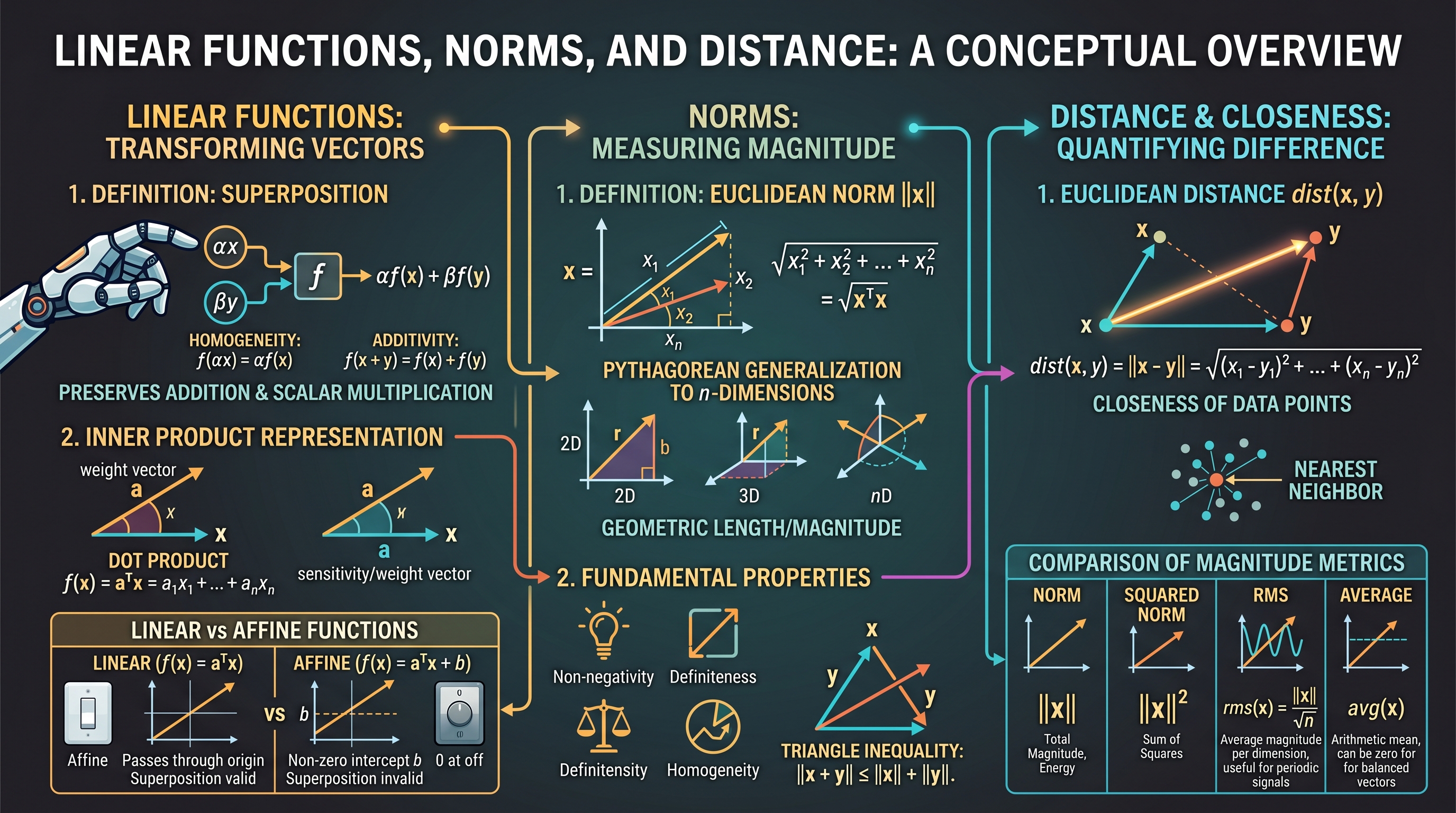
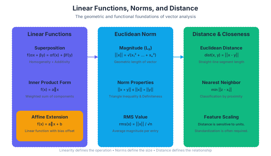
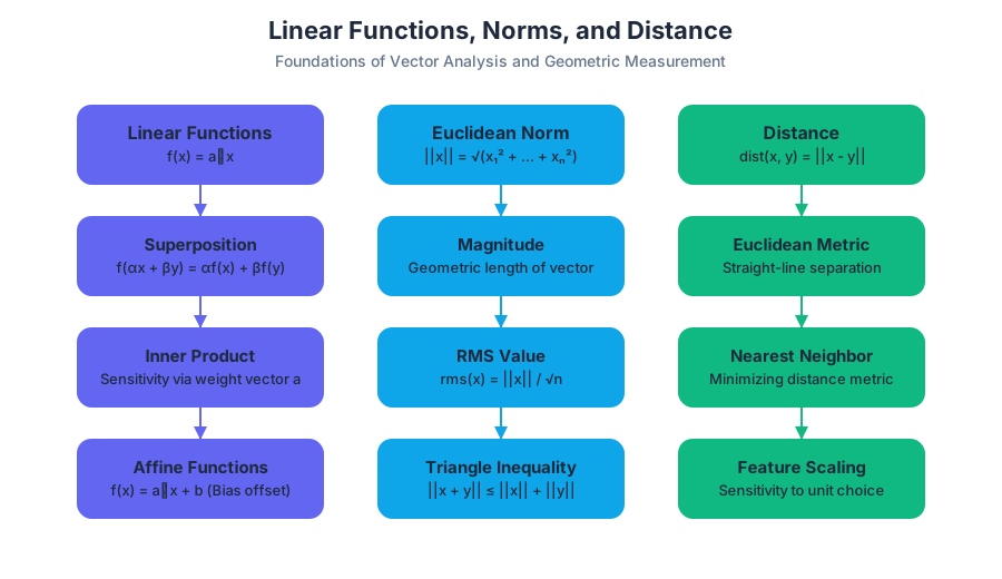
A function $f: \mathbb{R}^n \to \mathbb{R}$ is considered linear if it preserves the operations of addition and scalar multiplication. This is captured by the superposition property, which is the defining characteristic of linearity in any system.
The Superposition Property
The principle of superposition states that the response of a linear system to a weighted sum of inputs is the same as the weighted sum of the responses to those individual inputs. Mathematically, a function $f$ is linear if for all vectors $x, y$ and all scalars $\alpha, \beta$:
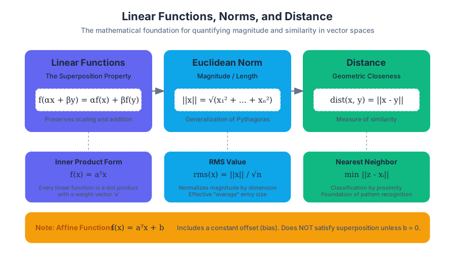
Definition: Superposition $$f(\alpha x + \beta y) = \alpha f(x) + \beta f(y)$$
This property can be decomposed into two distinct requirements:
- Homogeneity: $f(\alpha x) = \alpha f(x)$ (scaling the input scales the output).
- Additivity: $f(x + y) = f(x) + f(y)$ (the output of a sum is the sum of the outputs).
Inner Product Representation
One of the most profound results in finite-dimensional linear algebra is that every linear function $f: \mathbb{R}^n \to \mathbb{R}$ can be expressed as an inner product with some fixed vector $a$. This means that for any linear function, there exists a unique vector $a$ such that: $$f(x) = a^Tx = a_1x_1 + a_2x_2 + \dots + a_nx_n$$ In this context, the vector $a$ is often called the weight vector or the coefficient vector. Each component $a_i$ represents the sensitivity of the function's output to changes in the corresponding input $x_i$.
Affine Functions
In practice, many functions we encounter are not strictly linear but are affine. An affine function is a linear function plus a constant offset: $$f(x) = a^Tx + b$$ where $b$ is a scalar called the bias or offset. While affine functions do not satisfy the superposition property (unless $b=0$), they are often colloquially referred to as "linear" in fields like regression and neural networks.
| Feature | Linear Function ($f(x) = a^Tx$) | Affine Function ($f(x) = a^Tx + b$) |
|---|---|---|
| Passes through origin? | Yes ($f(0) = 0$) | No (unless $b=0$) |
| Superposition? | Valid | Invalid |
| Homogeneity? | Valid | Invalid |
| Additivity? | Valid | Invalid |
| Constant Term? | Always 0 | Any real number $b$ |
The Euclidean Norm
While the inner product gives us a way to relate two vectors, the norm gives us a way to measure a single vector. The Euclidean norm (also known as the $L_2$ norm) is the standard geometric measure of a vector's "length" or "magnitude."
Definition and Calculation
The Euclidean norm of an $n$-vector $x$ is denoted by $|x|$ and is defined as the square root of the sum of the squares of its components:
Definition: Euclidean Norm $$|x| = \sqrt{x_1^2 + x_2^2 + \dots + x_n^2} = \sqrt{x^Tx}$$
This definition is a direct generalization of the Pythagorean theorem from 2D and 3D space to $n$-dimensional space.
Fundamental Properties of Norms
For any vector $x$ and scalar $\alpha$, the Euclidean norm satisfies several critical properties:
- Non-negativity: $|x| \ge 0$.
- Definiteness: $|x| = 0$ if and only if $x = 0$.
- Homogeneity: $|\alpha x| = |\alpha| |x|$.
- Triangle Inequality: $|x + y| \le |x| + |y|$.
Root Mean Square (RMS) Value
In many engineering applications, particularly those involving periodic signals or large datasets, the norm can become very large as the dimension $n$ increases. To normalize for the number of components, we use the RMS value: $$rms(x) = \frac{|x|}{\sqrt{n}} = \sqrt{\frac{x_1^2 + \dots + x_n^2}{n}}$$ The RMS value provides a measure of the "typical" size of an entry in the vector. For example, if a vector represents a voltage signal over time, the RMS value represents the effective constant voltage that would deliver the same power.
| Metric | Formula | Interpretation |
|---|---|---|
| Norm $|x|$ | $\sqrt{\sum x_i^2}$ | Total magnitude / "Length" |
| Squared Norm $|x|^2$ | $\sum x_i^2$ | Energy / Sum of Squares |
| RMS $rms(x)$ | $|x| / \sqrt{n}$ | Average magnitude per dimension |
| Average $avg(x)$ | $(\sum x_i) / n$ | Arithmetic mean (can be zero for large $x$) |
Distance and Closeness
The concept of "distance" allows us to quantify how similar or different two vectors are. In the Euclidean framework, the distance between two vectors $x$ and $y$ is simply the norm of their difference.
Euclidean Distance
The distance $dist(x, y)$ is defined as: $$dist(x, y) = |x - y| = \sqrt{(x_1 - y_1)^2 + \dots + (x_n - y_n)^2}$$ This represents the length of the straight-line segment connecting the points $x$ and $y$ in $n$-dimensional space.
Applications: Nearest Neighbor Classification
Distance is the fundamental metric used in Nearest Neighbor (NN) algorithms. Given a set of "training" vectors $x_1, \dots, x_N$ with known labels, and a new "test" vector $z$, the NN algorithm finds the training vector $x_i$ that minimizes $|z - x_i|$.
- Feature Vectors: In this context, vectors represent "features" of an object (e.g., height, weight, age).
- Scaling: It is crucial to note that distance is sensitive to the units of the components. If one component is measured in millimeters and another in kilometers, the kilometer-scale component will dominate the distance calculation. This necessitates feature scaling or standardization.
The Cauchy-Schwarz Inequality
The Cauchy-Schwarz inequality is one of the most important inequalities in all of mathematics. It relates the inner product of two vectors to the product of their norms.
Theorem: Cauchy-Schwarz Inequality For any $n$-vectors $a$ and $b$: $$|a^Tb| \le |a| |b|$$
Implications and Equality Conditions
The inequality tells us that the absolute value of the inner product can never exceed the product of the lengths of the vectors.
- Equality: The equality $|a^Tb| = |a| |b|$ holds if and only if $a$ and $b$ are linearly dependent (i.e., one is a scalar multiple of the other, $a = \beta b$ or $b = \beta a$).
- Upper Bound: It provides a way to bound the output of a linear function. If $f(x) = a^Tx$, then $|f(x)| \le |a| |x|$.
The Triangle Inequality
A direct consequence of the Cauchy-Schwarz inequality is the Triangle Inequality: $$|x + y| \le |x| + |y|$$ Geometrically, this states that the length of one side of a triangle cannot exceed the sum of the lengths of the other two sides. In the context of vectors, it means that the "shortcut" (the vector sum $x+y$) is always shorter than or equal to the path taken by traveling along $x$ and then along $y$.
| Inequality | Mathematical Statement | Geometric/Physical Meaning |
|---|---|---|
| Cauchy-Schwarz | $ | x^Ty |
| Triangle Inequality | $|x+y| \le |x| + |y|$ | The straight line is the shortest path. |
| Reverse Triangle | $|x-y| \ge | |x| - |y| |
Angles and Orthogonality
By combining the inner product and the norm, we can define the angle between two vectors in $\mathbb{R}^n$, extending our 3D intuition to arbitrary dimensions.
Defining the Angle
The angle $\theta$ between two non-zero vectors $a$ and $b$ is defined as: $$\cos \theta = \frac{a^Tb}{|a| |b|}$$ Because of the Cauchy-Schwarz inequality, the term on the right is always between $-1$ and $1$, ensuring that a unique angle $\theta \in [0, \pi]$ always exists.
Orthogonality
Two vectors are said to be orthogonal if their inner product is zero: $$a^Tb = 0 \iff a \perp b$$ In geometric terms, orthogonal vectors are at a $90^\circ$ angle to each other. This is a central concept in linear algebra, leading to the development of orthonormal bases and projections.
Correlation Coefficient
In statistics, the correlation coefficient $\rho$ between two vectors of data (with zero mean) is exactly the cosine of the angle between them.
- If $\theta = 0$ ($\cos \theta = 1$), the vectors are perfectly correlated.
- If $\theta = \pi$ ($\cos \theta = -1$), the vectors are perfectly negatively correlated.
- If $\theta = \pi/2$ ($\cos \theta = 0$), the vectors are uncorrelated (orthogonal).
Common Pitfalls and Misconceptions
Even experienced practitioners can stumble on the nuances of norms and linear functions.
- Linear vs. Affine Confusion: In many software libraries (like scikit-learn), a "Linear Regression" model actually fits an affine function ($y = ax + b$). Forgetting the bias term $b$ in a purely linear model can lead to poor fits if the data does not pass through the origin.
- The "Square Root" Oversight: When calculating the Euclidean norm, beginners often forget to take the square root of the sum of squares, resulting in the squared norm $|x|^2$. While the squared norm is useful (and computationally cheaper), it does not satisfy the triangle inequality or the homogeneity property of a true norm.
- Dimensionality and Distance: In very high dimensions, the concept of "distance" becomes counter-intuitive. In a phenomenon known as the curse of dimensionality, the distance between any two random points in a high-dimensional cube tends to become almost equal, making "nearest neighbor" searches less effective.
- RMS vs. Average: The RMS value is always greater than or equal to the absolute value of the average. $rms(x) \ge |avg(x)|$. Using the average to describe the "magnitude" of a signal like a sine wave is useless (as the average is zero), whereas the RMS provides the correct physical context of power.
Summary of Key Formulas
| Concept | Formula |
|---|---|
| Linear Function | $f(x) = a^Tx$ |
| Euclidean Norm | $|x| = \sqrt{\sum x_i^2}$ |
| RMS Value | $rms(x) = |x| / \sqrt{n}$ |
| Distance | $dist(x, y) = |x - y|$ |
| Cauchy-Schwarz | $ |
| Angle ($\theta$) | $\cos \theta = (x^Ty) / (|x| |y|)$ |
Clustering and Linear Independence
Key concepts: K-means algorithm · Linear independence · Basis · Orthonormal vectors · Gram-Schmidt algorithm
Introduces the K-means algorithm for data grouping and the concept of linear independence and bases.
Clustering and Linear Independence
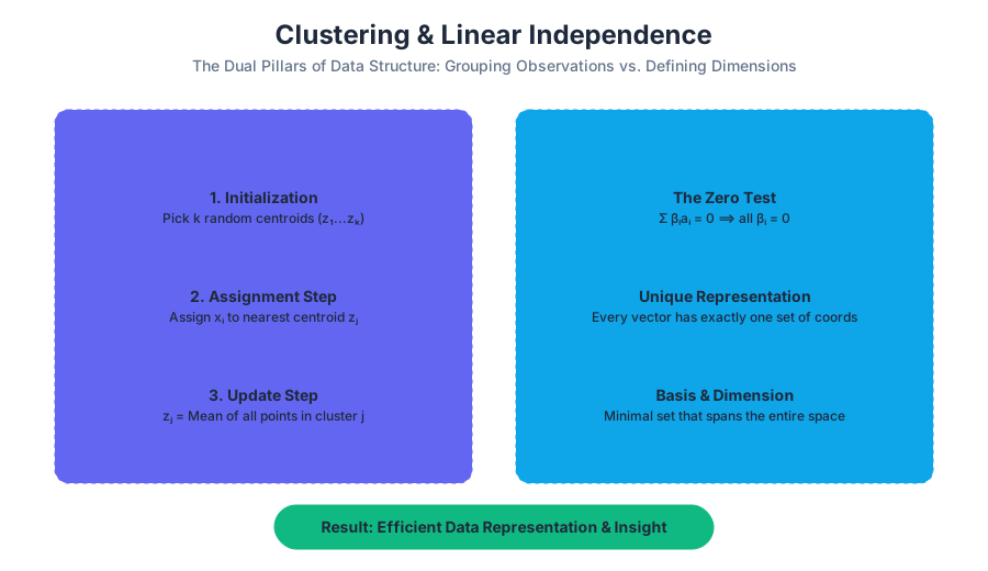
In the landscape of applied linear algebra, the transition from raw data to actionable insight requires two fundamental pillars: a method for discovering latent structure (Clustering) and a rigorous framework for defining the "dimensions" of a data space (Linear Independence). While clustering allows us to group similar observations, linear independence and the resulting concept of a basis allow us to decompose and reconstruct those observations without redundancy.
K-Means Clustering: The Geometry of Grouping
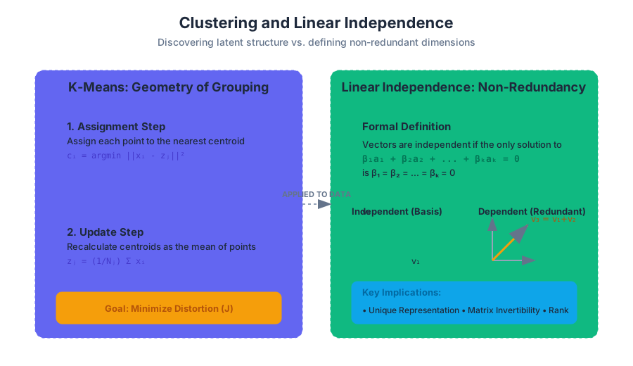
At its core, clustering is the task of partitioning a set of $N$ vectors $x_1, \dots, x_N$ into $k$ groups or "clusters." The goal is to ensure that vectors within the same group are closer to each other than they are to vectors in other groups. This is the foundational problem of unsupervised learning.
What it is
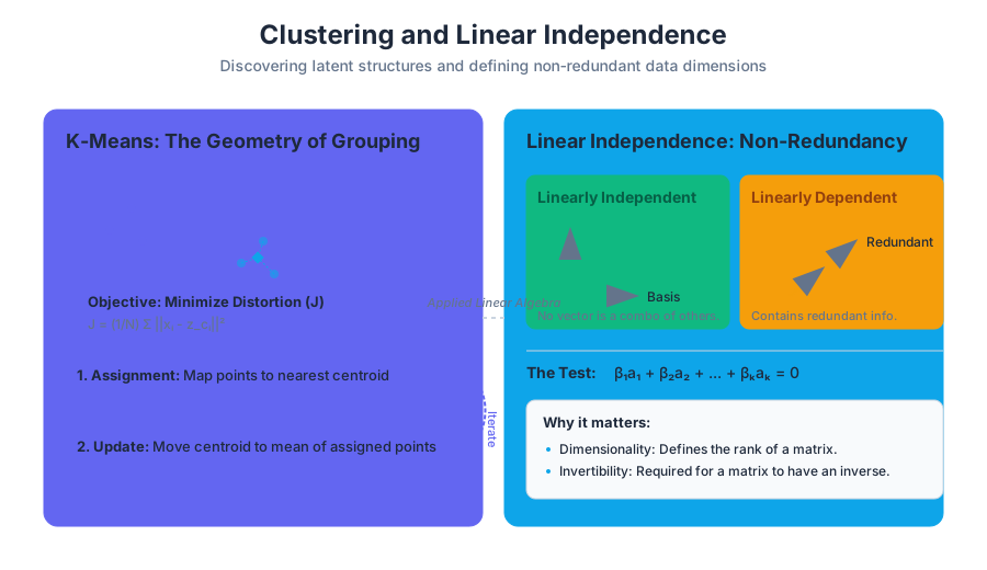
The K-means algorithm (often referred to as Lloyd’s algorithm) is an iterative procedure used to minimize the clustering objective (or distortion), which is the mean squared distance from each data point to its assigned cluster representative.
Mathematically, we seek to find:
- Assignments: $c_1, \dots, c_N \in {1, \dots, k}$, where $c_i$ is the index of the cluster to which $x_i$ is assigned.
- Representatives: $z_1, \dots, z_k$, which are the "centroids" of each cluster.
The objective function $J$ is defined as: $$J = \frac{1}{N} \sum_{i=1}^N |x_i - z_{c_i}|^2$$
Why it matters
Clustering is the "Swiss Army Knife" of data science. It is used for:
- Customer Segmentation: Grouping users by behavior for targeted marketing.
- Data Compression: Representing a large set of vectors by a small set of representatives (Vector Quantization).
- Feature Engineering: Using cluster assignments as inputs for other machine learning models.
- Anomaly Detection: Identifying points that are unusually far from any cluster representative.
How it works: Lloyd's Algorithm
The algorithm alternates between two steps until the assignments no longer change:
- Assignment Step: For each data point $x_i$, find the closest representative $z_j$ and assign $c_i = j$. $$c_i = \text{argmin}_{j=1, \dots, k} |x_i - z_j|^2$$
- Update Step: For each cluster $j$, compute the new representative $z_j$ as the mean of all points assigned to that cluster. $$z_j = \frac{1}{N_j} \sum_{i: c_i = j} x_i$$ where $N_j$ is the number of points in cluster $j$.
| Feature | Description |
|---|---|
| Input | A set of $N$ vectors and the number of clusters $k$. |
| Initialization | Randomly choose $k$ points or use K-means++. |
| Convergence | Guaranteed to reach a local minimum, but not necessarily the global minimum. |
| Complexity | $O(N \cdot k \cdot d \cdot i)$ where $d$ is dimension and $i$ is iterations. |
| Distance Metric | Typically Euclidean distance ($L_2$ norm). |
Concrete Example: K-Means in Python
The following implementation demonstrates the iterative nature of the algorithm using numpy.
import numpy as np

def k_means(X, k, max_iters=100):
    # 1. Initialization: Randomly pick k points from X as initial centroids
    centroids = X[np.random.choice(X.shape[0], k, replace=False)]

    for i in range(max_iters):
        # 2. Assignment Step: Compute distances and assign clusters
        # Distances: (N, k) matrix
        distances = np.linalg.norm(X[:, np.newaxis] - centroids, axis=2)
        labels = np.argmin(distances, axis=1)

        # 3. Update Step: Compute new centroids
        new_centroids = np.array([X[labels == j].mean(axis=0) for j in range(k)])

        # Check for convergence
        if np.all(centroids == new_centroids):
            break
        centroids = new_centroids

    return centroids, labels

# Example Usage
data = np.array([[1, 2], [1, 4], [1, 0], [10, 2], [10, 4], [10, 0]])
centers, assignments = k_means(data, k=2)
print(f"Centroids:\n{centers}")
Common Pitfalls
- The $k$ Problem: Choosing the right number of clusters is non-trivial. Using the "Elbow Method" (plotting $J$ vs. $k$) is a common heuristic.
- Local Minima: Since the algorithm is greedy, it can get stuck. Running the algorithm multiple times with different initializations (K-means++) is standard practice.
- Outliers: A single point very far from the rest can significantly pull the centroid away from the dense part of the cluster.
Linear Independence: The Logic of Non-Redundancy
If clustering is about finding patterns, linear independence is about the fundamental "ingredients" of a vector space. It tells us whether a set of vectors contains redundant information.
What it is
A set of $k$ vectors $a_1, \dots, a_k$ is linearly independent if the only way to form the zero vector using a linear combination of these vectors is to set all coefficients to zero.
Definition: The vectors $a_1, \dots, a_k$ are linearly independent if: $$\beta_1 a_1 + \beta_2 a_2 + \dots + \beta_k a_k = 0 \implies \beta_1 = \beta_2 = \dots = \beta_k = 0$$
If there exists a set of coefficients (not all zero) that results in the zero vector, the set is linearly dependent. This means at least one vector in the set can be expressed as a linear combination of the others.
Why it matters
Linear independence is the gatekeeper for several critical concepts:
- Dimensionality: A set of $n$ independent $n$-vectors is enough to reach any point in $\mathbb{R}^n$.
- Unique Representation: If a set of vectors is independent, any vector in their span can be represented by exactly one unique set of coefficients.
- Invertibility: In matrix algebra, a square matrix is invertible if and only if its columns are linearly independent.
Comparison: Independent vs. Dependent Sets
| Property | Linearly Independent | Linearly Dependent |
|---|---|---|
| Redundancy | Zero redundancy; every vector adds a new dimension. | Contains at least one redundant vector. |
| Zero Vector | Cannot form $0$ unless all weights are $0$. | Can form $0$ with non-zero weights. |
| Span | Spans a space of dimension $k$. | Spans a space of dimension $< k$. |
| Geometric Intuition | Vectors point in "different" directions. | At least one vector lies in the "plane" of others. |
The Independence-Dimension Inequality
A crucial theorem in linear algebra states that if a set of $k$ vectors in $\mathbb{R}^n$ is linearly independent, then $k$ must be less than or equal to $n$.
- If $k > n$, the set must be linearly dependent.
- You cannot have 4 independent vectors in a 3D space.
Basis and Orthonormal Vectors
When a set of vectors is both linearly independent and spans a particular space, we call it a basis. However, not all bases are created equal. In engineering and physics, we prefer bases that are "clean"—where every vector is at a right angle to the others and has a length of one.
What it is: Orthonormal Sets
A set of vectors $q_1, \dots, q_k$ is orthonormal if:
- Orthogonal: Every pair of distinct vectors has an inner product of zero ($q_i^T q_j = 0$ for $i \neq j$).
- Normalized: Every vector has a norm (length) of one ($|q_i| = 1$).
The Orthonormal Advantage: If $q_1, \dots, q_k$ are orthonormal, they are automatically linearly independent.
Why it matters
Orthonormal bases simplify calculations immensely. To find the coefficients of a vector $x$ in an orthonormal basis $q_1, \dots, q_n$, you don't need to solve a system of equations. You simply use the inner product: $$x = (q_1^T x)q_1 + (q_2^T x)q_2 + \dots + (q_n^T x)q_n$$ The coefficient for $q_i$ is just the projection of $x$ onto $q_i$.
| Basis Type | Orthogonal? | Unit Length? | Independence? |
|---|---|---|---|
| Standard Basis ($e_i$) | Yes | Yes | Yes |
| General Basis | No | No | Yes |
| Orthogonal Basis | Yes | No | Yes |
| Orthonormal Basis | Yes | Yes | Yes |
The Gram-Schmidt Algorithm: Constructing Orthogonality
How do we take a "messy" set of linearly independent vectors and turn them into a "clean" orthonormal basis? We use the Gram-Schmidt process.
How it works
Given independent vectors $a_1, \dots, a_k$, we produce orthonormal vectors $q_1, \dots, q_k$ through a process of successive projection and subtraction.
The Algorithm Steps:
- Step 1: Take the first vector $a_1$ and normalize it. $$\tilde{q}_1 = a_1, \quad q_1 = \tilde{q}_1 / |\tilde{q}_1|$$
- Step 2: Take $a_2$, subtract its projection onto $q_1$ (to make it orthogonal), then normalize. $$\tilde{q}_2 = a_2 - (q_1^T a_2)q_1, \quad q_2 = \tilde{q}_2 / |\tilde{q}_2|$$
- Step $i$: Take $a_i$, subtract its projections onto all previously calculated $q_1, \dots, q_{i-1}$, then normalize. $$\tilde{q}i = a_i - \sum{j=1}^{i-1} (q_j^T a_i)q_j, \quad q_i = \tilde{q}_i / |\tilde{q}_i|$$
Gram-Schmidt Complexity and Logic
| Step Component | Mathematical Operation | Purpose |
|---|---|---|
| Projection | $(q_j^T a_i)q_j$ | Finds the "shadow" of $a_i$ on the existing basis. |
| Orthogonalization | $a_i - \text{projections}$ | Removes the parts of $a_i$ that are already "covered." |
| Normalization | $\tilde{q}_i / |\tilde{q}_i|$ | Ensures the resulting vector has unit length. |
| Failure Case | $|\tilde{q}_i| = 0$ | Occurs if and only if the input vectors were linearly dependent. |
Concrete Example: Gram-Schmidt in Python
This implementation follows the "Classical Gram-Schmidt" (CGS) approach.
import numpy as np

def gram_schmidt(A):
    """
    Returns an orthonormal basis for the columns of A.
    A: (n, k) matrix where columns are independent vectors.
    """
    n, k = A.shape
    Q = np.zeros((n, k))

    for i in range(k):
        # Start with the original vector
        v = A[:, i]

        # Subtract projections onto all previous vectors in Q
        for j in range(i):
            v = v - np.dot(Q[:, j], A[:, i]) * Q[:, j]

        # Normalize the resulting vector
        norm = np.linalg.norm(v)
        if norm < 1e-10:
            raise ValueError("Vectors are linearly dependent.")
        Q[:, i] = v / norm

    return Q

# Example
A = np.array([[1.0, 1.0], [1.0, 0.0], [0.0, 1.0]])
Q = gram_schmidt(A)
print(f"Orthonormal Basis Q:\n{Q}")
print(f"Check Orthogonality (Q^T Q):\n{np.dot(Q.T, Q)}")
Common Pitfalls in Gram-Schmidt
- Numerical Instability: In floating-point arithmetic, the "Classical" Gram-Schmidt (shown above) can lose orthogonality due to rounding errors. The Modified Gram-Schmidt (MGS) algorithm is more stable and is used in professional libraries like LAPACK.
- Linear Dependence: If the input vectors are not independent, the algorithm will eventually produce a zero vector $\tilde{q}_i$, making normalization (division by zero) impossible.
Synthesis: Connecting Clustering and Independence
While they seem like disparate topics, clustering and linear independence often interact in high-dimensional data analysis.
- Dimensionality Reduction: Before clustering, we often use techniques like Principal Component Analysis (PCA). PCA relies on finding an orthonormal basis (eigenvectors) that captures the most variance. We project data onto this basis to reduce noise before running K-means.
- Rank and Clusterability: If a dataset of 1,000 points actually lies on a 2D plane in a 100D space, the "rank" of the data matrix is only 2. This linear dependence (or near-dependence) tells us that the data is highly structured, making it a prime candidate for clustering.
- The Centroid Space: The representatives $z_1, \dots, z_k$ found by K-means define a subspace. The linear independence of these centroids determines whether the clusters are truly distinct or if some clusters are redundant "mixtures" of others.
Summary of Key Formulas
| Concept | Formula / Property |
|---|---|
| K-means Objective | $J = \frac{1}{N} \sum |x_i - z_{c_i}|^2$ |
| Linear Independence | $\sum \beta_i a_i = 0 \implies \beta_i = 0$ |
| Orthogonality | $q_i^T q_j = 0$ |
| Gram-Schmidt Step | $q_i = \text{unit}(a_i - \sum \text{proj}_{q_j} a_i)$ |
Matrix Basics and Geometric Examples
Key concepts: Transpose · Matrix-vector multiplication · Incidence matrix · Convolution
Defines matrix dimensions, multiplication with vectors, and applications in geometry and graph theory.
Matrix Basics and Geometric Examples
In the landscape of applied linear algebra, a matrix is far more than a static rectangular grid of numbers. It is a linear operator—a mathematical machine that transforms vectors from one space to another. While a vector represents a point or a direction in $n$-dimensional space, a matrix represents a relationship between spaces. This section explores the fundamental mechanics of matrices, their geometric interpretations, and their specialized applications in graph theory and signal processing.
The Matrix as a Linear Operator
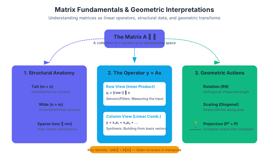
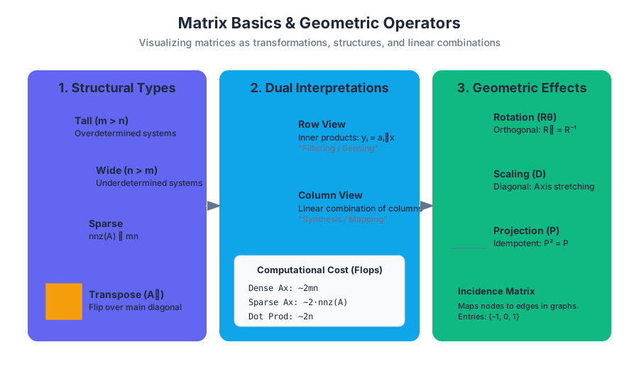
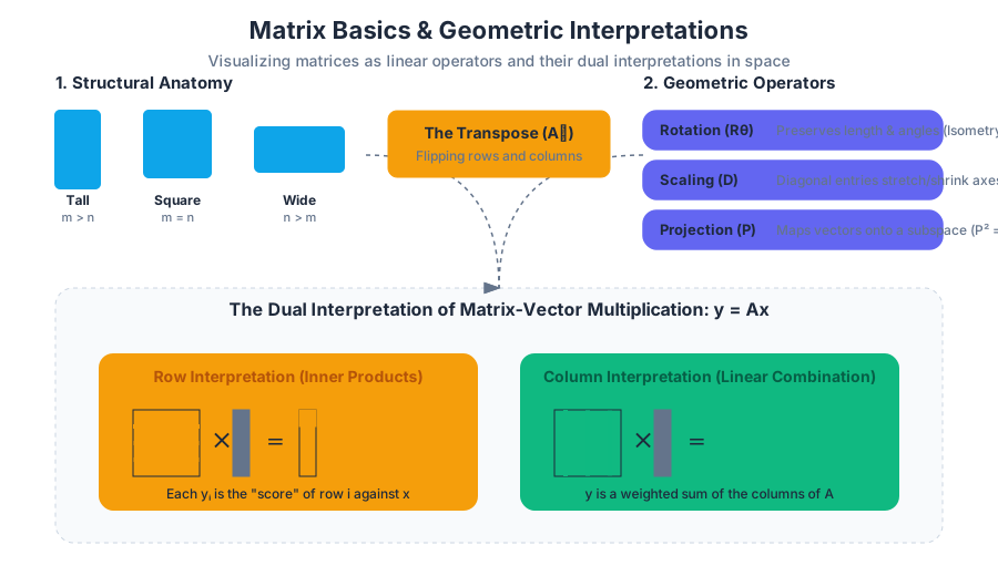
A matrix $A \in \mathbb{R}^{m \times n}$ consists of $m$ rows and $n$ columns. We refer to $m \times n$ as the dimensions of the matrix. If $m = n$, the matrix is square; if $m > n$, it is tall; and if $n > m$, it is wide.
Definition: A matrix $A$ is a collection of $n$ vectors $a_1, \dots, a_n \in \mathbb{R}^m$ arranged side-by-side: $$A = [a_1 \quad a_2 \quad \dots \quad a_n]$$ Alternatively, it can be viewed as a stack of $m$ row vectors.
Matrix Anatomy and Types
Understanding the structure of a matrix is the first step in determining the efficiency of the algorithms applied to it.
| Matrix Type | Condition | Significance |
|---|---|---|
| Square | $m = n$ | Represents transformations within the same dimensional space. |
| Tall | $m > n$ | Often represents overdetermined systems (more equations than variables). |
| Wide | $n > m$ | Often represents underdetermined systems (more variables than equations). |
| Sparse | $nnz(A) \ll mn$ | Most entries are zero; allows for specialized, high-speed computation. |
| Diagonal | $A_{ij} = 0$ for $i \neq j$ | Represents simple scaling along the axes. |
The Transpose Operation
The transpose of a matrix $A$, denoted $A^T$, is the matrix obtained by flipping $A$ over its main diagonal. Formally, $(A^T){ij} = A{ji}$.
Why it Matters
The transpose is not merely a reorientation of data; it is fundamental to the concept of duality. In optimization and physical systems, if $A$ represents a transformation from input to output, $A^T$ often represents the relationship between the sensitivities or forces in the reverse direction.
Mechanics and Properties
The transpose satisfies several algebraic identities that are essential for deriving complex linear models:
- $(A^T)^T = A$
- $(A + B)^T = A^T + B^T$
- $(\alpha A)^T = \alpha A^T$
- $(AB)^T = B^T A^T$ (Note the reversal of order)
Common Pitfalls
A frequent mistake is assuming that $A^T A = A A^T$. This is only true for normal matrices. For a tall matrix $A$, $A^T A$ is an $n \times n$ matrix (often the Gram matrix), while $A A^T$ is a much larger $m \times m$ matrix.
Matrix-Vector Multiplication
The operation $y = Ax$ is the cornerstone of linear algebra. It can be interpreted in two distinct, equally important ways.
1. The Row Interpretation (Inner Products)
In this view, each entry $y_i$ of the resulting vector is the inner product of the $i$-th row of $A$ with the vector $x$: $$y_i = \sum_{j=1}^n A_{ij} x_j$$ This perspective is useful when $A$ represents a set of sensors or filters, and $x$ is the input signal. Each $y_i$ is the "score" or "response" of the $i$-th filter to the input.
2. The Column Interpretation (Linear Combination)
This is the "geometric" view favored in modern data science. Here, $y$ is a linear combination of the columns of $A$, weighted by the entries of $x$: $$y = x_1 a_1 + x_2 a_2 + \dots + x_n a_n$$ This tells us that $y$ lies in the span of the columns of $A$. If $x$ is a vector of coefficients, $Ax$ is the process of synthesizing a new signal from the basis vectors stored in $A$.
Complexity and Performance
The computational cost of matrix-vector multiplication is a key constraint in large-scale systems.
| Operation | Flops (Floating Point Operations) |
|---|---|
| Inner product ($n$-vector) | $2n - 1$ |
| $Ax$ (where $A \in \mathbb{R}^{m \times n}$) | $\approx 2mn$ |
| $Ax$ (where $A$ is sparse) | $\approx 2 \cdot nnz(A)$ |
Geometric Transformations in 2D and 3D
Matrices act as geometric operators. By multiplying a vector (representing a point) by a specific matrix, we can rotate, scale, or project that point.
Scaling and Reflection
A diagonal matrix $D$ scales space along the principal axes. If $D = \text{diag}(2, 0.5)$, every $x$-coordinate doubles, and every $y$-coordinate is halved. Reflection across the $y$-axis is achieved by the matrix: $$ \text{Ref}_y = \begin{bmatrix} -1 & 0 \ 0 & 1 \end{bmatrix} $$
Rotation
To rotate a vector in $\mathbb{R}^2$ counter-clockwise by an angle $\theta$, we use the rotation matrix: $$ R_\theta = \begin{bmatrix} \cos \theta & -\sin \theta \ \sin \theta & \cos \theta \end{bmatrix} $$ This matrix is orthogonal, meaning $R_\theta^T = R_\theta^{-1}$, which implies that rotation preserves the length of vectors (isometry).
Projections
A projection matrix $P$ maps a vector onto a subspace. For example, projecting onto the $x$-axis in 2D: $$ P_x = \begin{bmatrix} 1 & 0 \ 0 & 0 \end{bmatrix} $$ Note that $P^2 = P$. Once you have projected a point onto a line, projecting it again changes nothing.
The Incidence Matrix
In graph theory and network analysis, the incidence matrix $A$ is a mathematical representation of a directed graph. It maps the relationship between $n$ nodes and $m$ edges.
Definition and Construction
For a graph with $n$ nodes and $m$ directed edges, the incidence matrix $A \in \mathbb{R}^{n \times m}$ is defined as:
- $A_{ij} = 1$ if edge $j$ enters node $i$.
- $A_{ij} = -1$ if edge $j$ leaves node $i$.
- $A_{ij} = 0$ otherwise.
Physical Interpretation: Flow and Potential
The incidence matrix is the bridge between local interactions (edges) and global states (nodes).
- Flow Conservation ($Ax = s$): If $x$ is a vector of flows on each edge, then $Ax$ is a vector where each entry $(Ax)_i$ represents the net flow out of node $i$. If $(Ax)_i = 0$, the node satisfies Kirchhoff's Current Law (flow in = flow out).
- Potential Difference ($v = A^T u$): If $u$ is a vector of potentials at each node (e.g., voltage or pressure), then $A^T u$ is a vector of potential differences across each edge.
Example: A Simple Triangle Graph
Consider a graph with 3 nodes and 3 edges forming a triangle:
- Edge 1: Node 1 $\to$ Node 2
- Edge 2: Node 2 $\to$ Node 3
- Edge 3: Node 3 $\to$ Node 1
The incidence matrix $A$ would be: $$ A = \begin{bmatrix} -1 & 0 & 1 \ 1 & -1 & 0 \ 0 & 1 & -1 \end{bmatrix} $$
| Feature | Interpretation in $Ax = b$ |
|---|---|
| Rows | Represent nodes; sum of row entries is always 0. |
| Columns | Represent edges; each column has exactly one $1$ and one $-1$. |
| Nullspace | The vector $\mathbf{1}$ (all ones) is always in the nullspace of $A^T$. |
Convolution as a Matrix Operation
Convolution is a fundamental operation in signal processing and deep learning. While often defined using a sliding window summation, it can be elegantly represented as a matrix-vector multiplication.
The Toeplitz Structure
When we convolve a signal $x$ with a filter $h$, we are essentially performing a weighted moving average. This can be written as $y = Hx$, where $H$ is a Toeplitz matrix. A Toeplitz matrix has the property that each descending diagonal from left to right is constant.
Example: 1D Moving Average
Suppose we have a 3-point moving average filter $h = [1/3, 1/3, 1/3]$. For an input signal $x \in \mathbb{R}^4$, the convolution (with zero padding) can be represented as: $$ \begin{bmatrix} y_1 \ y_2 \ y_3 \ y_4 \end{bmatrix} = \begin{bmatrix} 1/3 & 0 & 0 & 0 \ 1/3 & 1/3 & 0 & 0 \ 1/3 & 1/3 & 1/3 & 0 \ 0 & 1/3 & 1/3 & 1/3 \end{bmatrix} \begin{bmatrix} x_1 \ x_2 \ x_3 \ x_4 \end{bmatrix} $$
Why it Matters in Deep Learning
In Convolutional Neural Networks (CNNs), the "convolution" layer is actually a cross-correlation operation. However, the principle remains: the layer applies a sparse, weight-shared matrix to the input data. The sparsity and the Toeplitz-like structure allow CNNs to learn local features with far fewer parameters than a "fully connected" (dense) matrix.
Summary of Matrix Operations
To wrap up the basics, we compare the primary ways matrices interact with vectors and other matrices.
| Operation | Mathematical Form | Primary Application |
|---|---|---|
| Transformation | $y = Ax$ | Computer graphics, robotics, coordinate shifts. |
| System of Equations | $Ax = b$ | Solving for unknowns, engineering statics. |
| Change of Basis | $x = B\tilde{x}$ | Data compression (PCA), frequency analysis (DFT). |
| Graph Mapping | $b = Ax$ | Network flow, circuit analysis, logistics. |
| Filtering | $y = Hx$ | Audio processing, image blurring, trend extraction. |
Common Pitfalls in Matrix Basics
- Dimension Mismatch: The most common error in matrix-vector multiplication $Ax$ is attempting to multiply an $m \times n$ matrix by a vector of size $m$. The vector must be size $n$ (matching the number of columns).
- Non-Commutativity: In matrix-matrix multiplication, $AB \neq BA$ in general. Geometrically, this means the order of transformations matters—rotating then translating is not the same as translating then rotating.
- Interpreting Zero Net Flow: In incidence matrices, a net flow of zero at a node doesn't mean there is no activity; it means the system is in steady-state equilibrium.
- Transpose of a Product: Forgetting to reverse the order: $(AB)^T = B^T A^T$. This is vital when calculating gradients in machine learning (the "Backpropagation" rule).
Linear Equations and Dynamical Systems
Key concepts: Affine functions · Systems of linear equations · State-space model · Population dynamics
Covers the representation of systems of equations and the modeling of time-varying states.
Linear Equations and Dynamical Systems
The transition from static vector operations to the study of Linear Equations and Dynamical Systems represents the shift from data representation to functional modeling. In this domain, we move beyond simply storing numbers in arrays to understanding how those numbers interact through transformations and how they evolve over time. By leveraging the structured properties of matrices, we can solve complex systems of constraints and predict the trajectory of physical, economic, and biological systems with high precision.
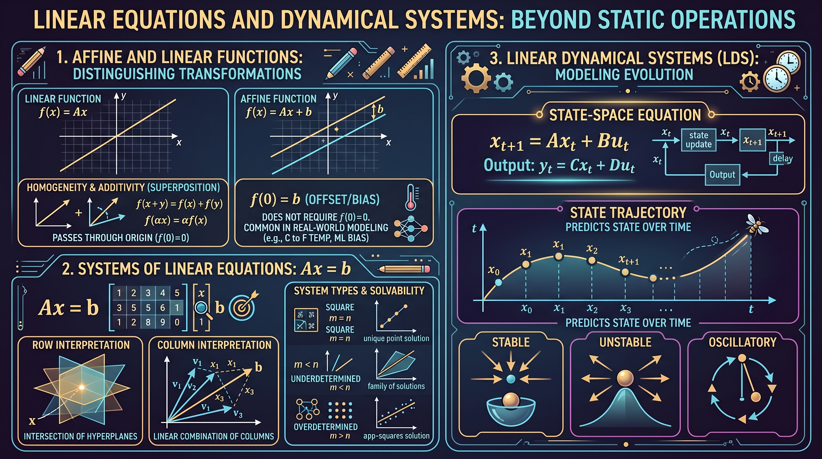
1. Affine and Linear Functions
At the core of linear modeling is the distinction between Linear Functions and Affine Functions. While often used interchangeably in casual conversation, their mathematical distinction is critical for accurate system modeling, particularly in data fitting and control theory.
What it is
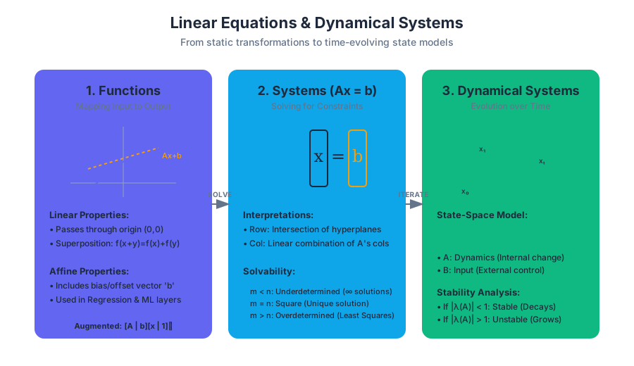
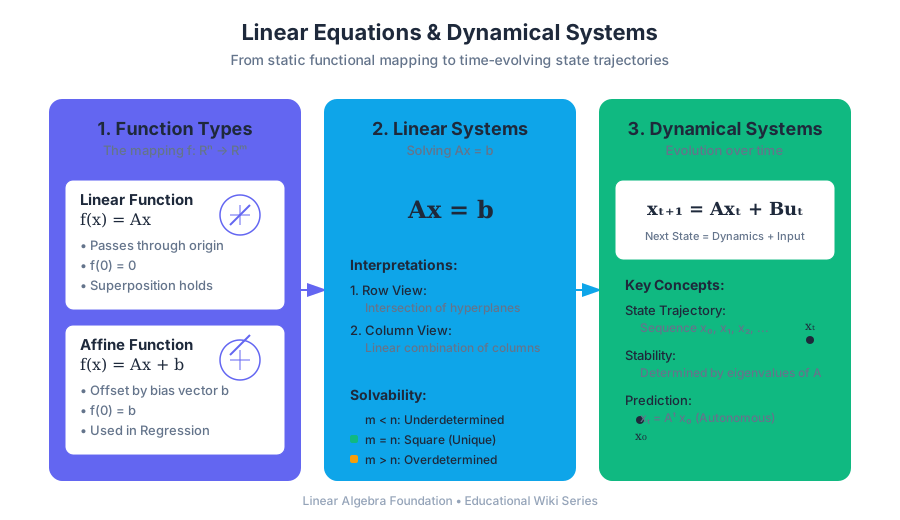
A function $f: \mathbb{R}^n \to \mathbb{R}^m$ is linear if it satisfies the properties of homogeneity and additivity (superposition). Mathematically, $f(x) = Ax$ for some matrix $A$. An affine function is a linear function plus a constant offset.
Definition: Affine Function A function $f: \mathbb{R}^n \to \mathbb{R}^m$ is affine if it can be expressed in the form: $$f(x) = Ax + b$$ where $A$ is an $m \times n$ matrix and $b$ is an $m$-vector (the offset or bias).
Why it matters
Most real-world relationships are not strictly linear; they do not pass through the origin $(0,0)$. For example, a temperature conversion from Celsius to Fahrenheit is affine ($F = 1.8C + 32$), not linear. In machine learning, the "weights" represent the linear transformation $A$, while the "bias" represents the affine offset $b$.
How it works
- Linearity Check: A function is linear if $f(0) = 0$. If $f(0) \neq 0$, the function is affine.
- Superposition: Linear functions satisfy $f(\alpha x + \beta y) = \alpha f(x) + \beta f(y)$. Affine functions do not satisfy this unless the sum of coefficients $\alpha + \beta = 1$.
- Matrix Representation: Any linear function can be represented as a matrix-vector product. To represent an affine function as a pure matrix-vector product, we often use augmented coordinates (adding a 1 to the vector $x$).
Comparison of Function Types
| Property | Linear Function ($Ax$) | Affine Function ($Ax + b$) |
|---|---|---|
| Passes through origin? | Yes ($f(0) = 0$) | No (unless $b=0$) |
| Superposition? | Always | Only if weights sum to 1 |
| Complexity (FLOPs) | $2mn$ | $2mn + m$ |
| Common Use Case | Physical scaling, rotations | Regression, Neural Network layers |
2. Systems of Linear Equations
A system of linear equations is a collection of $m$ equations involving $n$ variables. This is the "bread and butter" of applied linear algebra, represented compactly as $Ax = b$.
What it is
The equation $Ax = b$ represents a search for a vector $x$ that, when transformed by the matrix $A$, results in the vector $b$.
The Fundamental Problem Given $A \in \mathbb{R}^{m \times n}$ and $b \in \mathbb{R}^m$, find $x \in \mathbb{R}^n$ such that: $$ \sum_{j=1}^n A_{ij}x_j = b_i, \quad i = 1, \dots, m $$
Why it matters
Solving $Ax=b$ is the computational engine behind GPS positioning, structural engineering, circuit analysis, and economic equilibrium models. It allows us to reverse-engineer a cause ($x$) from an effect ($b$) given a known mechanism ($A$).
Interpretations of $Ax = b$
- Row Interpretation: Each row of $A$ represents a hyperplane in $n$-dimensional space. The solution $x$ is the intersection point of all these hyperplanes.
- Column Interpretation: $Ax$ is a linear combination of the columns of $A$. We are looking for the weights $x_1, \dots, x_n$ that combine the columns to produce $b$.
Solvability and System Types
| System Type | Relation | Interpretation | Typical Outcome |
|---|---|---|---|
| Square | $m = n$ | Same number of equations and unknowns | Unique solution (usually) |
| Underdetermined | $m < n$ | More unknowns than equations | Infinitely many solutions |
| Overdetermined | $m > n$ | More equations than unknowns | No exact solution (requires Least Squares) |
Common Pitfalls
- Singularity: A square matrix $A$ might not have a solution if its columns are linearly dependent (the matrix is "singular").
- Ill-conditioning: Small changes in $b$ can lead to massive changes in $x$ if the matrix $A$ is nearly singular, leading to numerical instability.
3. Linear Dynamical Systems (LDS)
A Linear Dynamical System describes how a state vector $x$ evolves over discrete time steps. It is the primary tool for modeling systems that change, from the cooling of a coffee cup to the fluctuations of the stock market.
What it is
An LDS is defined by a state-space equation where the next state is a linear function of the current state.
State-Space Model (Discrete Time) $$x_{t+1} = Ax_t + Bu_t$$ Where:
- $x_t$: State vector at time $t$ (the "memory" of the system).
- $A$: Dynamics matrix (describes internal evolution).
- $u_t$: Input vector (external forces or control signals).
- $B$: Input matrix (how external forces affect the state).
Why it matters
Dynamical systems allow for prediction and control. If we know the current state $x_0$ and the dynamics $A$, we can predict the state at any future time $T$ by calculating $x_T = A^T x_0$.
How it works: The Trajectory
The sequence of states $x_0, x_1, x_2, \dots$ is called the trajectory of the system.
- Autonomous Systems: If there are no inputs ($u_t = 0$), the system is $x_{t+1} = Ax_t$.
- Evolution: The state at time $t$ is $x_t = A^t x_0$.
- Stability:
- If the eigenvalues of $A$ are all less than 1 in magnitude, the system is stable ($x_t \to 0$).
- If any eigenvalue is greater than 1, the system explodes ($x_t \to \infty$).
Components of a State-Space Model
| Component | Symbol | Role |
|---|---|---|
| State | $x_t$ | Minimum information needed to predict the future. |
| Dynamics Matrix | $A$ | Determines the "physics" or "rules" of the system. |
| Input | $u_t$ | External control (e.g., accelerator pedal, medicine dosage). |
| Output | $y_t$ | What we actually observe (often $y_t = Cx_t$). |
4. Population Dynamics: A Concrete Case Study
One of the most intuitive applications of LDS is Population Dynamics, specifically using the Leslie Matrix model to track age-structured populations.
The Scenario
Imagine a population of animals divided into three age groups: Young, Juvenile, and Adult. We want to model how this population changes every year.
The Mechanics
The state vector is $x_t = [x_{1,t}, x_{2,t}, x_{3,t}]^T$, representing the number of individuals in each group. The dynamics are governed by:
- Birth rates ($b_i$): How many offspring each group produces.
- Survival rates ($s_i$): The probability of moving to the next age group.
The matrix $A$ (Leslie Matrix) looks like this: $$ A = \begin{bmatrix} b_1 & b_2 & b_3 \ s_1 & 0 & 0 \ 0 & s_2 & 0 \end{bmatrix} $$
Worked Example
Suppose:
- Birth rates: $b_1=0, b_2=0.5, b_3=2.0$
- Survival rates: $s_1=0.8, s_2=0.5$
- Initial population: $x_0 = [100, 50, 20]^T$
Step 1: Calculate $x_1$ $$ x_1 = Ax_0 = \begin{bmatrix} 0 & 0.5 & 2.0 \ 0.8 & 0 & 0 \ 0 & 0.5 & 0 \end{bmatrix} \begin{bmatrix} 100 \ 50 \ 20 \end{bmatrix} = \begin{bmatrix} (0.5 \times 50) + (2 \times 20) \ 0.8 \times 100 \ 0.5 \times 50 \end{bmatrix} = \begin{bmatrix} 65 \ 80 \ 25 \end{bmatrix} $$
Step 2: Analysis The total population changed from 170 to 170. However, the distribution shifted. Over many iterations, the population will either stabilize to a specific age distribution or grow/shrink exponentially depending on the dominant eigenvalue of $A$.
Population Dynamics Parameters
| Parameter | Symbol | Impact on System |
|---|---|---|
| Fecundity | $b_i$ | Increases the first entry of $x_{t+1}$ (births). |
| Survivorship | $s_i$ | Shifts population from $x_i$ to $x_{i+1}$. |
| Growth Factor | $\lambda$ | The rate at which the total population scales per step. |
5. Computational Complexity and FLOPs
Understanding the cost of these operations is vital for large-scale engineering.
Matrix-Vector Multiplication
To compute $y = Ax$ where $A \in \mathbb{R}^{m \times n}$:
- Each of the $m$ rows requires $n$ multiplications and $n-1$ additions.
- Total FLOPs (Floating Point Operations) $\approx 2mn$.
Dynamical System Simulation
To simulate $T$ steps of an autonomous LDS $x_{t+1} = Ax_t$:
- Each step is one matrix-vector multiply ($2n^2$ flops).
- Total complexity: $O(T \cdot n^2)$.
Insight: Sparsity In many real-world systems (like power grids or social networks), the matrix $A$ is sparse (mostly zeros). If $A$ has only $nnz$ non-zero entries, the complexity drops to $O(T \cdot nnz)$, which is significantly faster.
6. Summary of Extensions
Linear equations and dynamical systems serve as the foundation for more advanced topics:
- Least Squares: When $Ax=b$ has no solution (overdetermined), we find $x$ that minimizes $|Ax - b|^2$.
- Control Theory: Finding a sequence of inputs $u_0, u_1, \dots$ to drive the state $x_T$ to a desired target.
- Markov Chains: A special case of LDS where $x_t$ represents probabilities and the columns of $A$ sum to 1.
- Linear Regression: An affine modeling problem where we solve for the matrix $A$ and bias $b$ given observed data.
Study Guide: Linear Equations and Dynamical Systems
1. Core Definitions
- Linear Function: $f(x) = Ax$. Must satisfy $f(0)=0$ and superposition.
- Affine Function: $f(x) = Ax + b$. A linear transformation plus a translation.
- State Vector ($x_t$): A vector representing the condition of a system at time $t$.
- Dynamics Matrix ($A$): A square matrix defining how the state transitions from $t$ to $t+1$.
2. Solving $Ax=b$
- If $A$ is invertible, $x = A^{-1}b$.
- If $A$ is overdetermined, use the Normal Equations: $x = (A^T A)^{-1} A^T b$.
- If $A$ is underdetermined, there are infinitely many solutions; we often seek the one with the minimum norm.
3. Dynamical System Properties
- Autonomous: $x_{t+1} = Ax_t$.
- Input-Driven: $x_{t+1} = Ax_t + Bu_t$.
- Stability: Determined by the eigenvalues of $A$. If $\max|\lambda_i| < 1$, the system is stable.
- Leslie Matrix: A specific LDS used in biology to model age-structured population growth.
4. Computational Efficiency
- Matrix-vector multiplication: $2mn$ flops.
- Sparse matrices significantly reduce the cost of simulating high-dimensional dynamical systems.
- Solving $Ax=b$ via Gaussian elimination or QR factorization typically costs $O(n^3)$ for an $n \times n$ matrix.
5. Common Pitfalls to Avoid
- Confusing linear and affine functions in models where the offset $b$ is non-zero.
- Ignoring the "curse of dimensionality" when the state vector $x$ becomes extremely large.
- Assuming a system is stable without checking the properties of the dynamics matrix $A$.
Matrix Multiplication and Inverses
Key concepts: Matrix multiplication · QR Factorization · Left and Right Inverses · Pseudo-inverse
Explains matrix-matrix multiplication, QR factorization, and the conditions for matrix invertibility.
Matrix Multiplication and Inverses
Overview
In the landscape of applied linear algebra, matrix multiplication and inversion represent the transition from static data structures to dynamic operations. While a vector might represent a state, a matrix represents a transformation—a "verb" that acts upon the "noun" of the vector. This section explores the mechanics of composing these transformations through multiplication and the sophisticated methods required to reverse them. We move beyond the elementary view of matrices as grids of numbers, treating them instead as operators, basis changes, and systems of linear equations.
Matrix Multiplication: The Composition of Operators
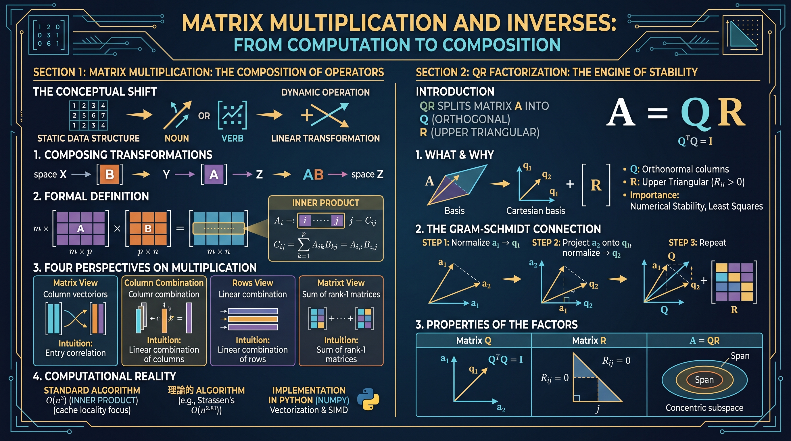
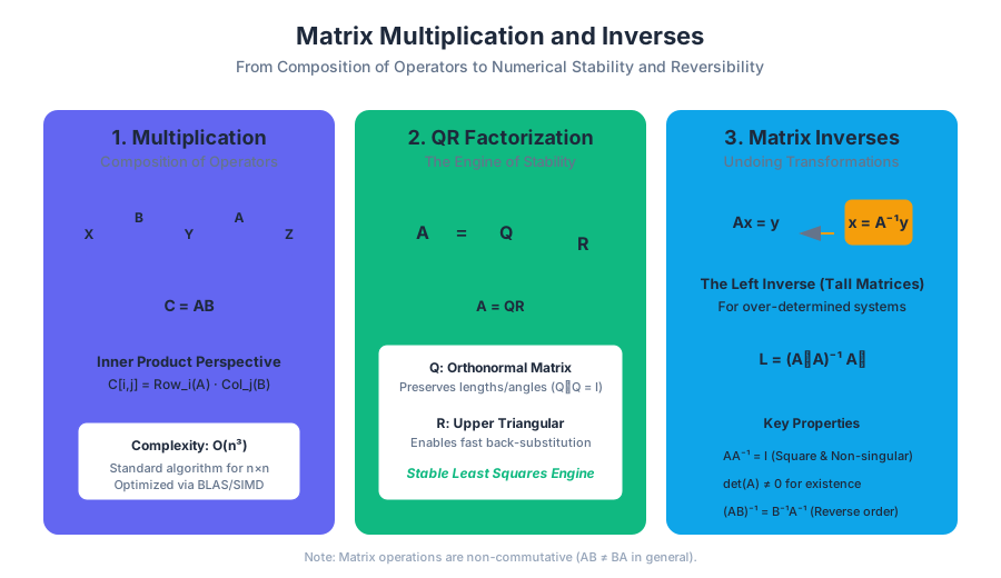
Matrix multiplication is the fundamental operation for composing linear transformations. If a matrix $B$ represents a transformation from space $\mathcal{X}$ to $\mathcal{Y}$, and a matrix $A$ represents a transformation from $\mathcal{Y}$ to $\mathcal{Z}$, then the product $C = AB$ represents the direct transformation from $\mathcal{X}$ to $\mathcal{Z}$.
1. Formal Definition
For an $m \times p$ matrix $A$ and a $p \times n$ matrix $B$, the product $C = AB$ is an $m \times n$ matrix. The entry in the $i$-th row and $j$-th column is defined as the inner product of the $i$-th row of $A$ and the $j$-th column of $B$:
Definition: Matrix-Matrix Product $$C_{ij} = \sum_{k=1}^{p} A_{ik}B_{kj} = A_{i,:} B_{:,j}$$ where $A_{i,:}$ is the $i$-th row of $A$ and $B_{:,j}$ is the $j$-th column of $B$.
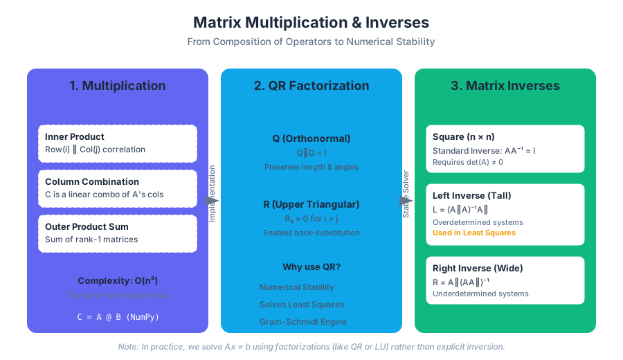
2. Four Perspectives on Multiplication
To truly master matrix multiplication, one must be able to switch between different mental models of the operation:
| Perspective | Mathematical View | Intuition |
|---|---|---|
| Inner Product | $C_{ij} = \text{row}_i(A) \cdot \text{col}_j(B)$ | Each entry is a correlation between a row and a column. |
| Column Combination | $\text{col}_j(C) = A \cdot \text{col}_j(B)$ | Each column of $C$ is a linear combination of the columns of $A$. |
| Row Combination | $\text{row}_i(C) = \text{row}_i(A) \cdot B$ | Each row of $C$ is a linear combination of the rows of $B$. |
| Outer Product Sum | $C = \sum_{k=1}^{p} A_{:,k} B_{k,:}$ | $C$ is the sum of $p$ rank-1 matrices. |
3. Computational Complexity
The standard algorithm for multiplying an $m \times p$ matrix by a $p \times n$ matrix requires $m \cdot n \cdot p$ multiplications and $m \cdot n \cdot (p-1)$ additions. In asymptotic notation, for square $n \times n$ matrices, this is $O(n^3)$. While theoretical algorithms like Strassen's ($O(n^{2.81})$) exist, the "inner product" approach optimized for cache locality remains the standard in high-performance libraries like BLAS (Basic Linear Algebra Subprograms).
4. Implementation in Python (NumPy)
In modern engineering, we rarely implement the triple-nested loop. Instead, we use vectorized libraries that leverage SIMD instructions.
import numpy as np

# Define two matrices
A = np.array([[1, 2], [3, 4]])
B = np.array([[5, 6], [7, 8]])

# Matrix multiplication (Operator @ or np.matmul)
C = A @ B

# Verification of the Row-Column rule for C[0,0]
# C[0,0] = A[0,0]*B[0,0] + A[0,1]*B[1,0] = 1*5 + 2*7 = 19
print(f"Resulting Matrix C:\n{C}")
assert C[0,0] == 19
QR Factorization: The Engine of Stability
QR Factorization is the decomposition of a matrix $A$ into the product of an orthogonal matrix $Q$ and an upper triangular matrix $R$. It is the practical workhorse behind solving least squares problems and eigenvalue computations.
1. What it is
For an $m \times n$ matrix $A$ with linearly independent columns, the QR factorization is: $$A = QR$$
- $Q$ ($m \times n$): Has orthonormal columns ($Q^TQ = I$).
- $R$ ($n \times n$): An upper triangular matrix with positive diagonal entries ($R_{ii} > 0$).
2. Why it matters
Solving systems via the standard inverse is numerically risky. $R$, being triangular, allows for back-substitution, which is computationally efficient and stable. $Q$, being orthonormal, preserves lengths and angles, ensuring that rounding errors do not explode during computation.
3. The Gram-Schmidt Connection
The QR factorization is essentially the Gram-Schmidt orthogonalization process recorded in matrix form.
- Take the first column of $A$ ($a_1$) and normalize it to get $q_1$.
- Take the second column ($a_2$), subtract its projection onto $q_1$, and normalize the result to get $q_2$.
- Repeat for all $n$ columns.
- The coefficients used to "build" the original $a_i$ from the new $q_i$ form the matrix $R$.
4. Properties of the Factors
| Matrix | Property | Significance |
|---|---|---|
| $Q$ | $Q^T Q = I$ | $Q$ is a rigid transformation (rotation/reflection). |
| $R$ | $R_{ij} = 0$ for $i > j$ | Encapsulates the "dependency" structure of the columns. |
| $A=QR$ | $\text{span}(a_1 \dots a_k) = \text{span}(q_1 \dots q_k)$ | $Q$ provides an orthonormal basis for the same space. |
Matrix Inverses: Undoing Transformations
The inverse of a matrix $A$, denoted $A^{-1}$, is a matrix that "reverses" the effect of $A$. If $Ax = y$, then $x = A^{-1}y$.
1. The Square Case (Standard Inverse)
A square matrix $A$ has an inverse if and only if it is non-singular (its determinant is non-zero, or it has full rank).
- $AA^{-1} = I$
- $A^{-1}A = I$
2. Left and Right Inverses
In many real-world applications (like sensor fusion or over-determined control), matrices are not square. We then look for "one-sided" inverses.
3. Left Inverse (Tall Matrices)
If $A$ is $m \times n$ with $m > n$ (more equations than variables) and has full column rank, it has a left inverse $L$ such that $LA = I_n$.
- Formula: $L = (A^T A)^{-1} A^T$
- Application: This is the core of the Least Squares solution. It finds the $x$ that minimizes $|Ax - b|^2$.
4. Right Inverse (Wide Matrices)
If $A$ is $m \times n$ with $m < n$ (more variables than equations) and has full row rank, it has a right inverse $R$ such that $AR = I_m$.
- Formula: $R = A^T (AA^T)^{-1}$
- Application: This is used for Minimum Norm problems. Among all $x$ that satisfy $Ax = b$, the right inverse finds the one with the smallest magnitude ($|x|$).
| Inverse Type | Shape | Condition | Formula ($A^\dagger$) | Result |
|---|---|---|---|---|
| Standard | Square ($n \times n$) | Full Rank | $A^{-1}$ | $AA^{-1} = A^{-1}A = I$ |
| Left | Tall ($m \times n$) | Full Col Rank | $(A^T A)^{-1} A^T$ | $A^\dagger A = I$ |
| Right | Wide ($m \times n$) | Full Row Rank | $A^T (AA^T)^{-1}$ | $AA^\dagger = I$ |
The Pseudo-inverse (Moore-Penrose)
When a matrix is singular or not square, the Moore-Penrose Pseudo-inverse ($A^\dagger$) provides a generalized solution. It is the unique matrix that satisfies four criteria (the Moore-Penrose conditions), the most intuitive being that $AA^\dagger A = A$ and $A^\dagger A A^\dagger = A^\dagger$.
1. Computation via QR
Using the QR factorization $A = QR$, the pseudo-inverse (for a full-rank tall matrix) can be computed as: $$A^\dagger = R^{-1} Q^T$$ This is significantly more stable than calculating $(A^TA)^{-1}A^T$ directly, as forming $A^TA$ squares the condition number of the problem, potentially doubling the loss of precision.
2. Numerical Example
Consider a simple tall matrix: $$A = \begin{bmatrix} 1 \ 2 \end{bmatrix}$$ The left inverse is: $$A^\dagger = (A^T A)^{-1} A^T = ([1, 2] \begin{bmatrix} 1 \ 2 \end{bmatrix})^{-1} [1, 2] = (5)^{-1} [1, 2] = [0.2, 0.4]$$ Verification: $$A^\dagger A = [0.2, 0.4] \begin{bmatrix} 1 \ 2 \end{bmatrix} = 0.2(1) + 0.4(2) = 1$$
Common Pitfalls and Engineering Considerations
1. The "Never Invert" Rule
In numerical computing, there is a famous adage: "Never compute the inverse of a matrix explicitly."
- Why? Computing $A^{-1}$ is more expensive and less stable than solving the system $Ax = b$ using decompositions like QR or LU.
- Exception: When you need to update the solution for many different $b$ vectors very quickly and can tolerate slight precision loss, or in specific theoretical derivations.
2. Rank Deficiency
If a matrix does not have full rank, $(A^TA)$ or $(AA^T)$ will be non-invertible (singular).
- Symptom: A "Singular Matrix" error in code.
- Solution: Use the Singular Value Decomposition (SVD) to compute the pseudo-inverse, which handles rank deficiency by zeroing out the singular values below a certain threshold.
3. Non-Commutativity
A frequent mistake is assuming $AB = BA$. In the context of transformations, this is obvious: rotating a cube then sliding it is not the same as sliding it then rotating it.
- Algebraic Trap: $(AB)^{-1} = B^{-1}A^{-1}$. Note the reversal of order. This is the "Shoes and Socks" principle: to undo the process of putting on socks then shoes, you must first take off the shoes, then the socks.
4. Complexity Comparison
| Operation | Complexity | Notes |
|---|---|---|
| Matrix-Vector Mult | $O(n^2)$ | Highly parallelizable. |
| Matrix-Matrix Mult | $O(n^3)$ | The bottleneck of deep learning. |
| QR Factorization | $O(mn^2)$ | Stable, used for Least Squares. |
| Inversion (Square) | $O(n^3)$ | Generally avoided in favor of solve. |
Summary of Connections
Matrix multiplication allows us to build complex models by stacking simpler ones. QR factorization provides the surgical precision needed to look inside those models and see which components are truly independent. Inverses and pseudo-inverses give us the power to work backward from observations to causes. Together, these tools form the mathematical backbone of everything from GPS positioning to the training of large language models.
The Least Squares Problem and Data Fitting
Key concepts: Residual norm · Normal equations · Feature engineering · Overfitting · Least squares classifier
Focuses on minimizing the residual norm and applying least squares to regression and classification.
The Least Squares Problem and Data Fitting
In the landscape of applied mathematics and engineering, few tools are as ubiquitous or as foundational as the Least Squares method. At its core, the least squares problem addresses a fundamental conflict: how do we "solve" a system of linear equations when no exact solution exists? This situation, known as an overdetermined system, occurs whenever we have more constraints (equations) than degrees of freedom (variables).
Whether it is a satellite determining its position from noisy GPS signals, a machine learning model predicting housing prices, or a control system stabilizing an aircraft, least squares provides the mathematical framework for finding the "best fit" solution by minimizing the discrepancy between observation and prediction.
1. The Least Squares Problem
The least squares problem is defined by an overdetermined system of linear equations $Ax = b$, where $A$ is an $m \times n$ matrix with $m > n$. In such cases, the vector $b$ is typically not in the range (column space) of $A$, meaning there is no $x$ such that $Ax$ exactly equals $b$.
1.1 The Residual Norm
To find the best approximation, we define the residual vector $r$, which represents the error between our prediction $Ax$ and the actual data $b$:
Definition: Residual Vector For a given $x$, the residual $r$ is defined as: $$r = Ax - b$$ The "size" of this error is measured using the Euclidean norm (or $L_2$ norm), and the goal of least squares is to find the $x$ that minimizes the square of this norm: $$\text{minimize } |Ax - b|^2 = \sum_{i=1}^m (a_i^T x - b_i)^2$$
By squaring the norm, we ensure the objective function is differentiable and penalize larger errors more heavily than smaller ones.
1.2 The Objective Function
The function $f(x) = |Ax - b|^2$ is a convex quadratic function. Because it is convex, any local minimum is also a global minimum. The point $\hat{x}$ that minimizes this function is called the least squares solution.
| Component | Symbol | Dimension | Description |
|---|---|---|---|
| Feature Matrix | $A$ | $m \times n$ | The data matrix containing $m$ observations and $n$ features. |
| Parameter Vector | $x$ | $n \times 1$ | The unknown coefficients we seek to estimate. |
| Target Vector | $b$ | $m \times 1$ | The observed outcomes or measurements. |
| Residual | $r$ | $m \times 1$ | The difference $Ax - b$; the "unexplained" part of the data. |
| Residual Norm | $|r|$ | Scalar | The total magnitude of error. |
2. The Normal Equations
To find the minimum of $|Ax - b|^2$, we can use multivariable calculus. By setting the gradient of the objective function with respect to $x$ to zero, we derive the Normal Equations.
2.1 Derivation and Mechanics
Expanding the squared norm gives: $$|Ax - b|^2 = (Ax - b)^T(Ax - b) = x^T A^T A x - 2b^T A x + b^T b$$
Taking the derivative with respect to $x$ and setting it to zero results in: $$2A^T A x - 2A^T b = 0$$ Which simplifies to the standard form of the normal equations:
The Normal Equations $$A^T A \hat{x} = A^T b$$ If the columns of $A$ are linearly independent, then the matrix $A^T A$ (the Gram matrix) is invertible, and the unique solution is: $$\hat{x} = (A^T A)^{-1} A^T b$$
2.2 Geometric Interpretation: The Orthogonality Principle
Geometrically, the least squares solution $\hat{x}$ has a profound property: the optimal residual vector $\hat{r} = A\hat{x} - b$ is orthogonal to the column space of $A$. This means that the error is perpendicular to every feature vector in our model. In other words, $A\hat{x}$ is the orthogonal projection of $b$ onto the subspace spanned by the columns of $A$.
3. Solving Least Squares in Practice
While the formula $\hat{x} = (A^T A)^{-1} A^T b$ is theoretically elegant, it is often numerically unstable to compute $(A^T A)^{-1}$ directly, especially if $A$ is "ill-conditioned" (meaning some columns are nearly linearly dependent).
3.1 QR Factorization
The preferred method for solving least squares in modern software is QR Factorization. We decompose $A$ into an $m \times n$ matrix $Q$ with orthonormal columns and an $n \times n$ upper triangular matrix $R$: $$A = QR$$
Substituting this into the normal equations: $$(QR)^T (QR) x = (QR)^T b$$ $$R^T Q^T Q R x = R^T Q^T b$$ Since $Q^T Q = I$ (identity matrix) and $R$ is invertible: $$R x = Q^T b$$
This system can be solved efficiently using back-substitution because $R$ is upper triangular.
| Method | Complexity (Flops) | Stability | Best For |
|---|---|---|---|
| Normal Equations | $n^2 m + \frac{1}{3}n^3$ | Lower | Small, well-conditioned problems. |
| QR Factorization | $2n^2 m - \frac{2}{3}n^3$ | High | General purpose, robust engineering. |
| SVD (Pseudo-inverse) | $O(mn^2)$ | Highest | Rank-deficient matrices (redundant features). |
import numpy as np

# Example: Solving Least Squares using NumPy
# A is 100x3 (100 observations, 3 features)
# b is 100x1 (100 targets)
A = np.random.randn(100, 3)
b = np.random.randn(100)

# Method 1: Direct solver (uses QR or SVD internally)
x_hat, residuals, rank, s = np.linalg.lstsq(A, b, rcond=None)

# Method 2: Manual Normal Equations (Not recommended for production)
x_normal = np.linalg.inv(A.T @ A) @ A.T @ b

print(f"Least Squares Coefficients: {x_hat}")
4. Data Fitting and Feature Engineering
Least squares is the engine behind Data Fitting, where we attempt to find a mathematical function $f(u)$ that maps an input $u$ to an output $y$.
4.1 From Linear to Non-linear Fitting
Even though the method is called "linear" least squares, it can fit highly non-linear relationships. The "linear" refers to the parameters $x$, not the input data $u$. We achieve this through feature engineering—transforming the raw input $u$ into a vector of features $a = \phi(u)$.
The model takes the form: $$y \approx x_1 \phi_1(u) + x_2 \phi_2(u) + \dots + x_n \phi_n(u)$$
4.2 Common Basis Functions
To fit complex data, we choose a set of basis functions that we believe represent the underlying physical or statistical process.
| Basis Type | Transformation $\phi(u)$ | Application |
|---|---|---|
| Linear | $[1, u]$ | Simple trend lines. |
| Polynomial | $[1, u, u^2, \dots, u^p]$ | Curves, non-linear growth. |
| Sinusoidal | $[\sin(u), \cos(u)]$ | Seasonal data, periodic signals. |
| Logarithmic | $[\log(u)]$ | Diminishing returns, saturation effects. |
| Radial Basis | $\exp(-|u - c|^2 / \sigma^2)$ | Localized fitting, non-parametric shapes. |
5. Overfitting and Validation
A common pitfall in data fitting is overfitting. This occurs when a model is so complex (e.g., a high-degree polynomial) that it fits the noise in the training data rather than the underlying pattern.
5.1 The Training vs. Test Split
To detect overfitting, we never evaluate a model solely on the data used to train it. Instead, we split our data into two or three sets:
- Training Set: Used to solve the least squares problem and find $\hat{x}$.
- Validation Set: Used to choose "hyperparameters," such as the degree of the polynomial or the number of features.
- Test Set: Used for a final, unbiased evaluation of the model's performance on unseen data.
5.2 Generalization Error
If the residual norm on the training set is very low, but the residual norm on the test set is very high, the model has failed to generalize.
Key Insight: The Complexity Tradeoff As model complexity (number of features $n$) increases:
- Training Error always decreases (or stays the same).
- Test Error initially decreases but eventually starts to increase as the model begins to "memorize" noise.
| Metric | Training Error | Test Error | Interpretation |
|---|---|---|---|
| High / High | High | High | Underfitting: Model is too simple. |
| Low / High | Low | High | Overfitting: Model is too complex/noisy. |
| Low / Low | Low | Low | Good Fit: Model has captured the pattern. |
6. The Least Squares Classifier
While least squares is primarily a regression tool (predicting continuous numbers), it can be adapted for classification (predicting categories).
6.1 Binary Classification
Suppose we want to classify data into two groups, labeled $+1$ and $-1$. We can fit a linear function $f(u) = a^T x + b$ such that:
- $f(u) \approx +1$ for class 1
- $f(u) \approx -1$ for class 2
To classify a new point $u$, we simply look at the sign of the prediction: $$\hat{y} = \text{sign}(a^T \hat{x} + \hat{b})$$
6.2 The Decision Boundary
The set of points where $a^T \hat{x} + \hat{b} = 0$ defines the decision boundary. For a 2D input, this is a line; for 3D, a plane; and for higher dimensions, a hyperplane. Points on one side are classified as positive, and points on the other as negative.
6.3 Multi-class Classification (One-vs-All)
To classify data into $K$ classes, we can train $K$ separate least squares classifiers. For each class $k$, we create a target vector $b^{(k)}$ where $b_i = 1$ if observation $i$ belongs to class $k$, and $b_i = -1$ otherwise. To classify a new point, we run it through all $K$ models and choose the class that yields the highest (most positive) value.
7. Common Pitfalls and Best Practices
- Ignoring the Intercept: Always include a "ones" column in your matrix $A$ (unless your data is centered). Without it, your model is forced to pass through the origin $(0,0)$, which rarely fits real-world data.
- Multi-collinearity: If two features are highly correlated (e.g., height in inches and height in centimeters), the matrix $A^T A$ becomes nearly singular. This leads to massive, unstable values in $\hat{x}$.
- Outliers: Because least squares minimizes the squared error, a single outlier (a data point very far from the rest) can pull the entire model toward it, ruining the fit for the majority of the data. In such cases, robust regression or $L_1$ minimization might be preferred.
- Feature Scaling: While theoretically not required for the basic least squares solution, scaling features to have similar ranges (e.g., between 0 and 1) is crucial for numerical stability and when adding regularization.
Summary of the Least Squares Pipeline
- Data Collection: Gather $m$ pairs of inputs $u_i$ and outputs $y_i$.
- Feature Engineering: Choose basis functions $\phi(u)$ to form the feature matrix $A$.
- Partitioning: Split data into training and test sets.
- Optimization: Solve $A^T A \hat{x} = A^T b$ using QR factorization on the training set.
- Validation: Evaluate the residual norm on the test set.
- Iteration: Adjust features or model complexity if the test error is too high.
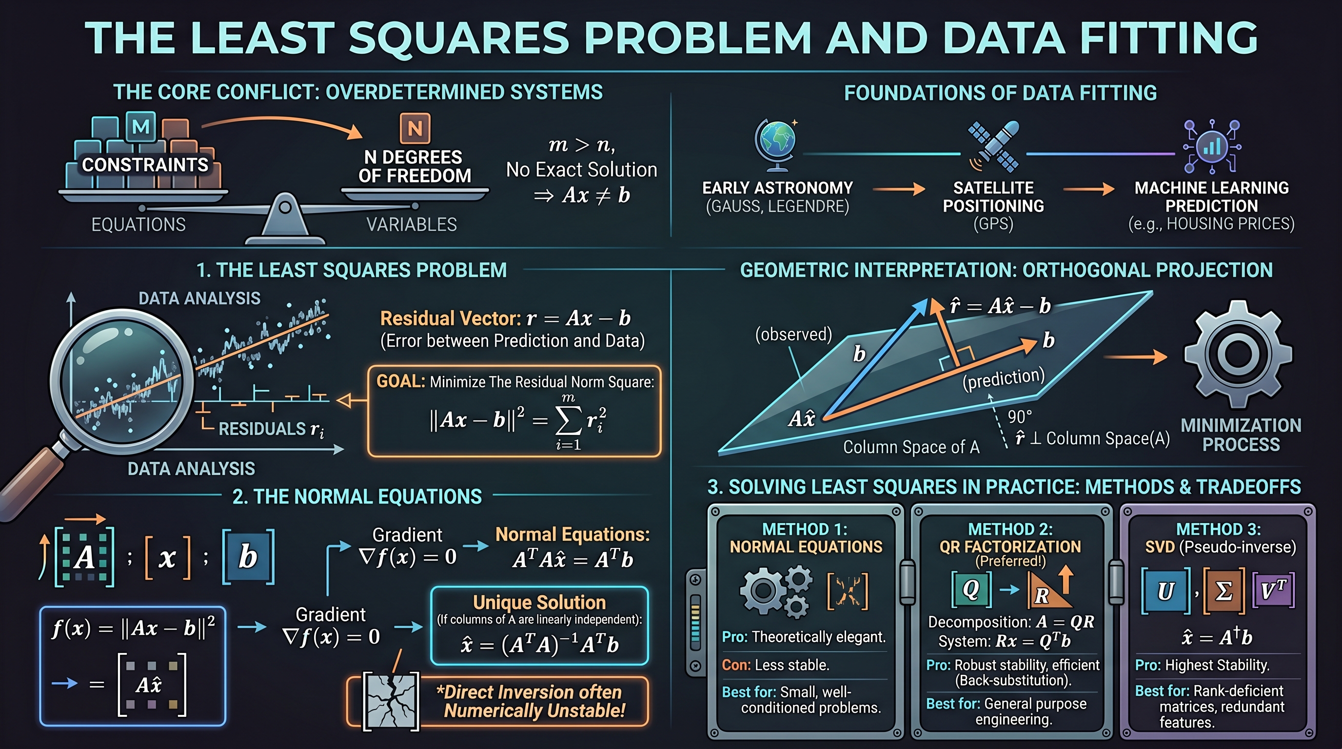
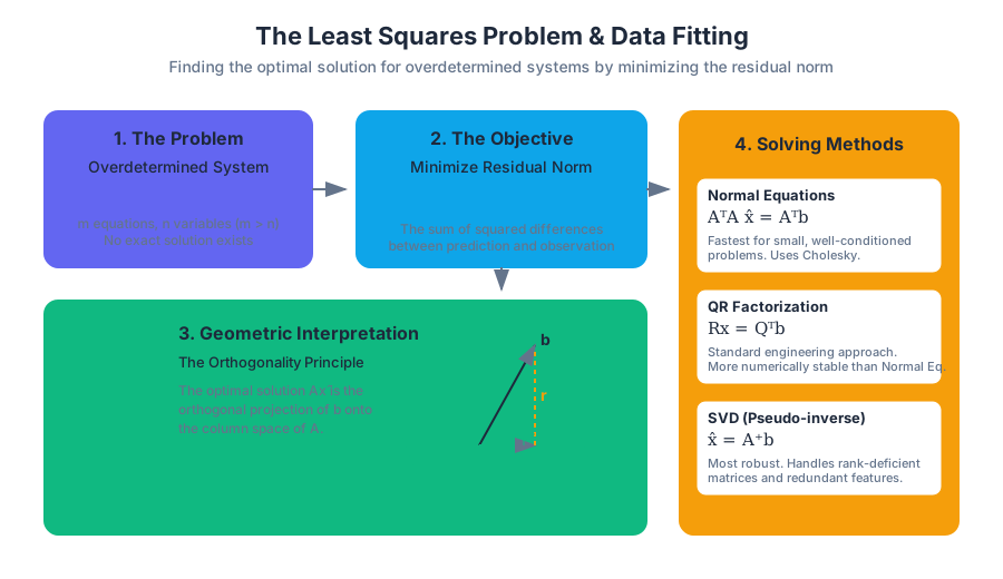
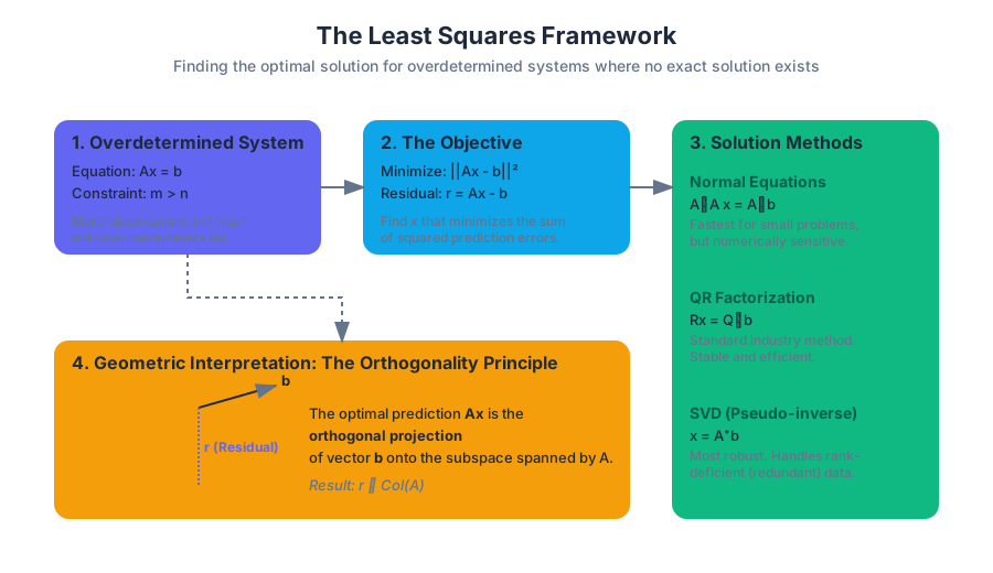
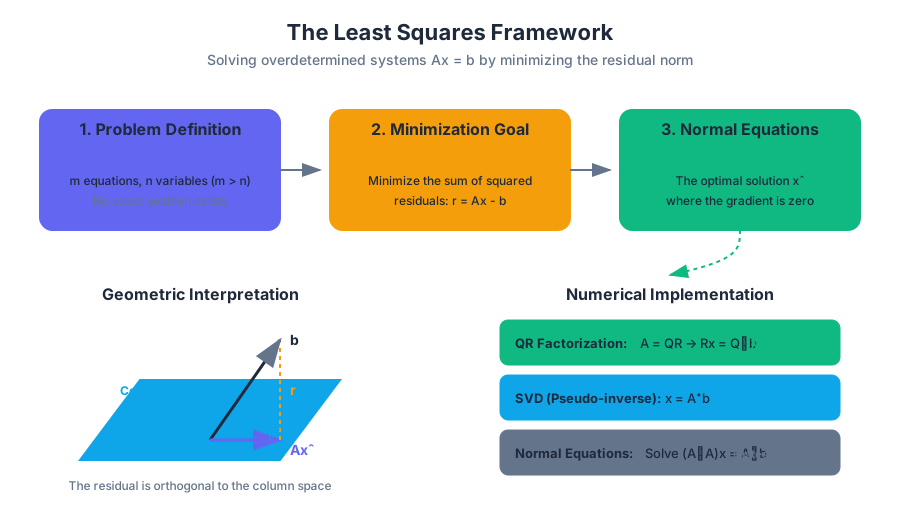
Regularization and Constrained Least Squares
Key concepts: Tikhonov regularization · Trade-off curves · KKT equations · Constrained least squares
Covers Tikhonov regularization for stability and solving least squares with equality constraints.
Regularization and Constrained Least Squares
In the pursuit of fitting models to data, the standard least squares approach—minimizing the sum of squared residuals—is often insufficient. While it provides the "best fit" in a purely algebraic sense, it frequently fails in the face of noisy data, collinear features, or physical requirements that the solution must satisfy. To address these challenges, we turn to Regularization and Constrained Least Squares. These techniques allow us to incorporate prior knowledge, ensure numerical stability, and manage the fundamental trade-off between model complexity and accuracy.
Tikhonov Regularization
Standard least squares seeks to minimize $|Ax - b|^2$. However, when the matrix $A$ is ill-conditioned (i.e., its columns are nearly linearly dependent) or when the number of parameters exceeds the number of observations, the resulting solution $x$ can have extremely large magnitudes. This phenomenon, often called "overfitting," results in a model that captures noise rather than the underlying signal.
Tikhonov regularization, also known as Ridge Regression or $L_2$ Regularization, addresses this by adding a penalty term to the objective function.
1. What it is
Tikhonov regularization modifies the least squares objective to include a weighted penalty on the norm of the solution vector $x$. The regularized objective function $J(x)$ is defined as:
Definition: Tikhonov Regularized Objective $$J(x) = |Ax - b|^2 + \lambda |x - x_{prior}|^2$$ Where $\lambda > 0$ is the regularization parameter and $x_{prior}$ is a suggested or "default" value for $x$ (often the zero vector).
In the most common case where $x_{prior} = 0$, the objective becomes: $$J(x) = |Ax - b|^2 + \lambda |x|^2$$
2. Why it matters
Regularization is the primary tool for solving ill-posed problems. It provides several critical benefits:
- Numerical Stability: It ensures that the matrix $(A^TA + \lambda I)$ is invertible, even if $A^TA$ is singular.
- Generalization: By penalizing large coefficients, it prevents the model from "chasing noise," leading to better performance on unseen data.
- Preference Incorporation: It allows the user to specify that the solution should be "small" or "smooth," which is a common physical or logical requirement.
3. How it works: The Augmented Matrix
One of the most elegant aspects of Tikhonov regularization is that it can be solved using the standard least squares machinery. We can reformulate the regularized problem as an augmented least squares problem.
To minimize $|Ax - b|^2 + \lambda |x|^2$, we define an augmented matrix $\tilde{A}$ and an augmented vector $\tilde{b}$: $$\tilde{A} = \begin{bmatrix} A \ \sqrt{\lambda}I \end{bmatrix}, \quad \tilde{b} = \begin{bmatrix} b \ 0 \end{bmatrix}$$
The problem then becomes minimizing $|\tilde{A}x - \tilde{b}|^2$. The normal equations for this augmented system are: $$(A^TA + \lambda I)x = A^Tb$$
| Feature | Standard Least Squares | Tikhonov Regularization |
|---|---|---|
| Objective | Minimize $|Ax - b|^2$ | Minimize $|Ax - b|^2 + \lambda |x|^2$ |
| Normal Equations | $A^TAx = A^Tb$ | $(A^TA + \lambda I)x = A^Tb$ |
| Invertibility | Requires $A$ to have full column rank | Guaranteed for any $\lambda > 0$ |
| Solution Norm | Can be very large | Controlled by $\lambda$ |
| Sensitivity to Noise | High | Low (Filtered) |
4. Concrete Example: Polynomial Interpolation
Imagine fitting a 10th-degree polynomial to 5 data points. A standard least squares fit will pass through every point perfectly but will oscillate wildly between them. By applying Tikhonov regularization with a small $\lambda$, we penalize the magnitude of the polynomial coefficients. This "flattens" the oscillations, resulting in a curve that captures the general trend of the data without over-fitting the specific noise in the 5 points.
5. Common Pitfalls
- Scaling Matters: Because the penalty $\lambda |x|^2$ treats all components of $x$ equally, it is crucial to scale the features (columns of $A$) so they have similar magnitudes. If one feature is measured in millimeters and another in kilometers, the regularization will disproportionately affect the one with the smaller numerical values.
- Bias-Variance Trade-off: Regularization introduces bias (the solution is no longer the "unbiased" minimum of the residuals) to reduce variance (sensitivity to the specific data sample). Choosing $\lambda$ too high will lead to "underfitting," where the model is too simple to capture the signal.
Trade-off Curves and the Pareto Frontier
The choice of the regularization parameter $\lambda$ is the central challenge in regularized least squares. It represents a fundamental trade-off between two competing goals: minimizing the residual norm (fit to data) and minimizing the solution norm (model complexity).
1. The Concept of Pareto Optimality
For any given $\lambda$, the resulting solution $x_\lambda$ is Pareto optimal. This means you cannot improve the fit (decrease $|Ax - b|$) without increasing the complexity (increasing $|x|$), and vice versa.
2. The L-Curve
When we plot the residual norm $|Ax_\lambda - b|$ against the solution norm $|x_\lambda|$ for a wide range of $\lambda$ values, we typically see an L-shaped curve.
- The Horizontal Part: Large $\lambda$. The solution norm is small, but the residual is very sensitive to changes in $\lambda$.
- The Vertical Part: Small $\lambda$. The residual is small, but the solution norm explodes as we try to fit the noise.
- The "Knee": The point of maximum curvature. This is often considered the "optimal" $\lambda$ as it balances both objectives effectively.
3. Parameter Sensitivity Table
| $\lambda$ Value | Residual $|Ax-b|$ | Solution Norm $|x|$ | Model Character |
|---|---|---|---|
| $\lambda \to 0$ | Minimum possible | Maximum (potentially $\infty$) | Overfit, unstable, high variance |
| Small $\lambda$ | Low | Moderate | Good balance (The "Knee") |
| Large $\lambda$ | High | Small | Underfit, biased, low variance |
| $\lambda \to \infty$ | $|b|$ | $0$ | Null model |
Constrained Least Squares
While regularization provides a "soft" penalty for violating a preference, Constrained Least Squares (CLS) enforces "hard" requirements that the solution must satisfy exactly. This is common in engineering, where physical laws (like conservation of mass or energy) must be obeyed.
1. What it is
The constrained least squares problem is defined as:
Definition: Constrained Least Squares Minimize $|Ax - b|^2$ Subject to $Cx = d$ Where $A \in \mathbb{R}^{m \times n}$, $b \in \mathbb{R}^m$, $C \in \mathbb{R}^{p \times n}$, and $d \in \mathbb{R}^p$.
We assume that the constraints are consistent (there exists at least one $x$ such that $Cx=d$) and that $C$ has full row rank (no redundant constraints).
2. Why it matters
CLS is essential when:
- Physical Constraints: A robotic arm must end at a specific coordinate ($Cx=d$) while moving in a way that minimizes energy expenditure ($|Ax-b|^2$).
- Prior Knowledge: In finance, a portfolio must have weights that sum to 1 ($\sum x_i = 1$).
- Nullspace Control: We want to find the best fit within a specific subspace of the parameter space.
3. How it works: The Method of Lagrange Multipliers
To solve this, we introduce a vector of Lagrange multipliers $z \in \mathbb{R}^p$ and define the Lagrangian function: $$L(x, z) = |Ax - b|^2 + z^T(Cx - d)$$
To find the minimum, we take the partial derivatives with respect to $x$ and $z$ and set them to zero.
- $\nabla_x L = 2A^T(Ax - b) + C^Tz = 0$
- $\nabla_z L = Cx - d = 0$
Rearranging these gives the system of linear equations that the optimal solution must satisfy.
The KKT Equations
The optimality conditions for the constrained least squares problem are known as the KKT (Karush-Kuhn-Tucker) equations. For linear equality constraints, these equations are both necessary and sufficient for a global minimum.
1. The KKT System
The KKT equations can be written as a single block-matrix equation: $$\begin{bmatrix} 2A^TA & C^T \ C & 0 \end{bmatrix} \begin{bmatrix} x \ z \end{bmatrix} = \begin{bmatrix} 2A^Tb \ d \end{bmatrix}$$
This matrix is often called the KKT Matrix. It is symmetric but indefinite, meaning it has both positive and negative eigenvalues. This makes it more challenging to solve numerically than the positive-definite systems found in standard least squares.
2. Solving the KKT System
There are three primary ways to solve this system:
- Direct Block Inversion: Solving the $(n+p) \times (n+p)$ system directly.
- Schur Complement: Solving for $z$ first, then $x$.
- $x = (A^TA)^{-1}(A^Tb - \frac{1}{2}C^Tz)$
- Substitute into $Cx=d$ to find $z$.
- Elimination Method: Using a basis for the nullspace of $C$ to transform the problem into an unconstrained one with fewer variables.
3. KKT Matrix Components
| Block | Dimension | Description |
|---|---|---|
| $2A^TA$ | $n \times n$ | The Hessian of the unconstrained objective |
| $C^T$ | $n \times p$ | The gradients of the constraints (Transposed) |
| $C$ | $p \times n$ | The constraint matrix |
| $0$ | $p \times p$ | Zero block (since constraints are linear) |
4. Variations: Weighted Constrained Least Squares
In some cases, we minimize a weighted norm $|Ax-b|_W^2$. The KKT system remains structurally the same, but the $A^TA$ block is replaced by $A^TWA$.
Comparison: Regularization vs. Constraints
It is helpful to view Tikhonov regularization and Constrained Least Squares as two sides of the same coin. In fact, they are mathematically linked via the concept of Duality.
The Equivalence Insight For every regularization parameter $\lambda$, there exists a constraint value $\epsilon$ such that minimizing $|Ax-b|^2$ subject to $|x|^2 \leq \epsilon$ yields the same solution as the Tikhonov problem.
| Feature | Tikhonov Regularization | Constrained Least Squares |
|---|---|---|
| Constraint Type | "Soft" (Penalty) | "Hard" (Equality) |
| Parameter | $\lambda$ (Weight of penalty) | $d$ (Target value) |
| Solution Method | Augmented Matrix / Normal Eqs | KKT System |
| Requirement | Minimizes a weighted sum | Satisfies $Cx=d$ exactly |
| Use Case | Preventing overfitting / Stability | Enforcing physical laws |
Worked Example: Minimum Norm Solution
A classic application of constrained least squares is finding the minimum norm solution to an underdetermined system of equations.
Problem: Suppose we have more variables than equations ($p < n$). We want to find the vector $x$ that satisfies $Cx = d$ while being as "small" as possible.
Formulation:
- Minimize $|x|^2$ (This is $|Ax-b|^2$ where $A=I$ and $b=0$)
- Subject to $Cx = d$
KKT Equations: $$\begin{bmatrix} 2I & C^T \ C & 0 \end{bmatrix} \begin{bmatrix} x \ z \end{bmatrix} = \begin{bmatrix} 0 \ d \end{bmatrix}$$
From the first row: $2x + C^Tz = 0 \implies x = -\frac{1}{2}C^Tz$. Substitute into the second row: $C(-\frac{1}{2}C^Tz) = d \implies -\frac{1}{2}CC^Tz = d$. Solving for $z$: $z = -2(CC^T)^{-1}d$. Substituting back for $x$: $$x = C^T(CC^T)^{-1}d$$
This is the famous pseudo-inverse solution for underdetermined systems. It represents the point in the solution space ${x \mid Cx=d}$ that is closest to the origin.
Extensions and Advanced Concepts
1. Generalized Tikhonov Regularization
Instead of penalizing $|x|^2$, we can penalize $|Dx|^2$ where $D$ is a differencing matrix. This is used in Tikhonov Regularization for Smoothing. If $D$ computes the first difference ($x_i - x_{i-1}$), the penalty encourages the solution to be "flat." If $D$ computes the second difference, it encourages "smoothness" (low curvature).
2. $L_1$ Regularization (Lasso)
While Tikhonov uses the $L_2$ norm, using the $L_1$ norm ($\sum |x_i|$) leads to sparse solutions where many components of $x$ are exactly zero. This is used for feature selection. Unlike $L_2$, $L_1$ regularization does not have a closed-form solution like the augmented matrix and requires iterative optimization.
3. Total Least Squares (TLS)
In standard LS, we assume errors only exist in the vector $b$. In Total Least Squares, we assume there are errors in both $A$ and $b$. This leads to a different regularization framework often solved via Singular Value Decomposition (SVD).
Common Pitfalls in Implementation
- Ignoring the Condition Number: Even with regularization, if $\lambda$ is extremely small, the matrix $(A^TA + \lambda I)$ can still be poorly conditioned. Always check the condition number of your system.
- Inconsistent Constraints: In CLS, if the constraints $Cx=d$ are contradictory (e.g., $x_1=1$ and $x_1=2$), the KKT system will have no solution. This often happens in large systems with redundant sensor data.
- Over-regularization: It is tempting to use a large $\lambda$ to get a very "clean" looking solution. However, this often washes away the actual signal you are trying to measure. Always validate against a hold-out test set.
- Numerical Precision in KKT: Because the KKT matrix is indefinite, standard Cholesky factorization cannot be used. One must use $LDL^T$ factorization or QR-based methods to ensure numerical stability.
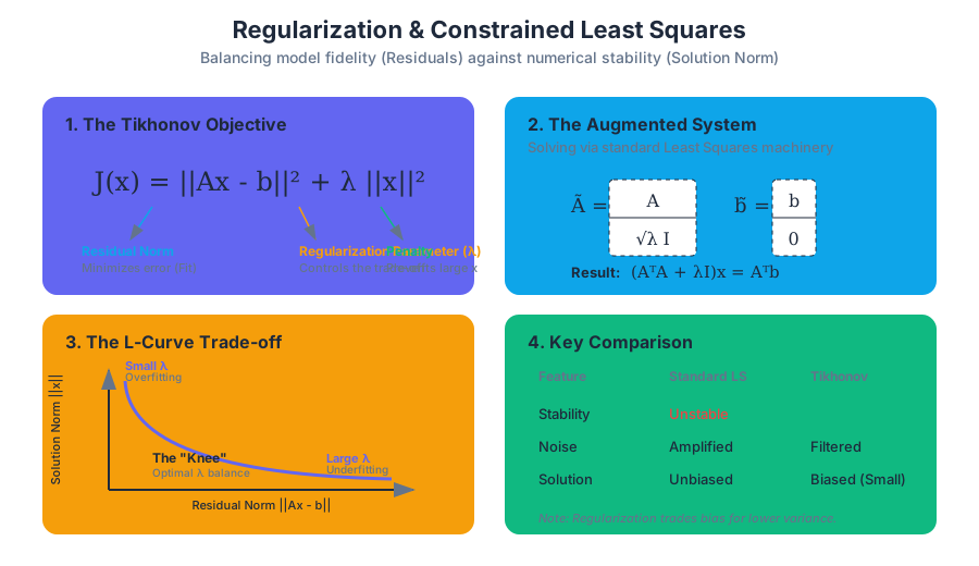
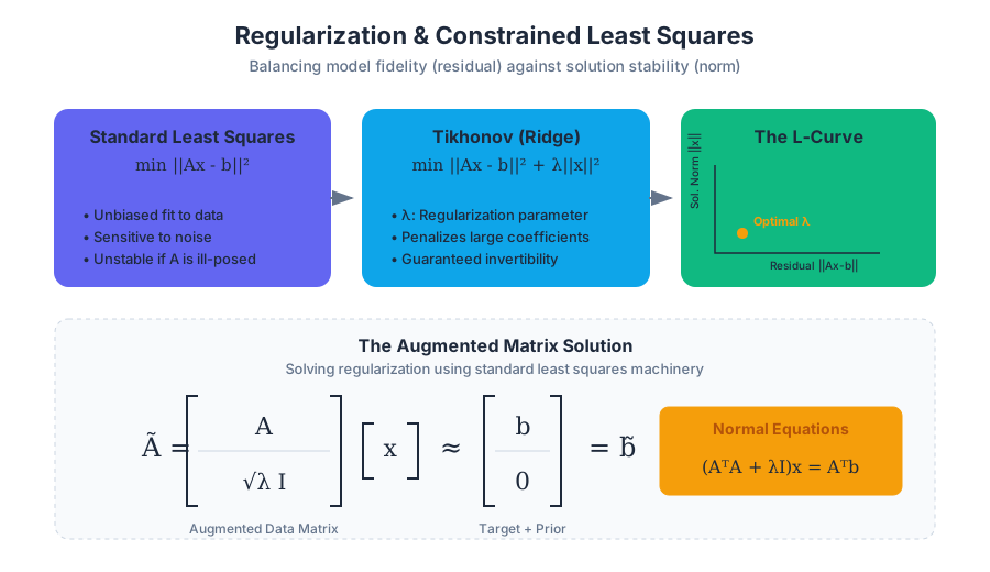
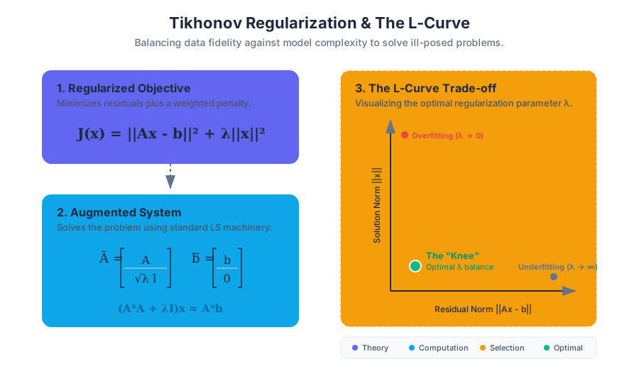
Nonlinear Least Squares
Key concepts: Gauss-Newton algorithm · Levenberg-Marquardt algorithm · Augmented Lagrangian · Penalty algorithm
Introduces iterative algorithms for solving least squares problems where the model is nonlinear.
Nonlinear Least Squares
In the landscape of mathematical optimization, Nonlinear Least Squares (NLS) represents the bridge between the simple, closed-form solutions of linear regression and the complex, iterative world of general non-convex optimization. While linear least squares can be solved in a single "shot" using the Normal Equations or QR factorization, NLS arises when the model function depends nonlinearly on the parameters. This is the standard regime for real-world problems ranging from satellite navigation (GPS) and computer vision (Structure from Motion) to pharmacokinetics and neural network training.
The Fundamental Problem
The goal of Nonlinear Least Squares is to find a parameter vector $x \in \mathbb{R}^n$ that minimizes the sum of the squares of the errors (residuals) between observed data and a nonlinear model.
Formally, we define the residual function $r: \mathbb{R}^n \to \mathbb{R}^m$ (where $m \geq n$): $$r(x) = \begin{bmatrix} r_1(x) \ r_2(x) \ \vdots \ r_m(x) \end{bmatrix}$$ The objective function to minimize is the squared $L_2$ norm of these residuals: $$f(x) = \frac{1}{2} |r(x)|^2_2 = \frac{1}{2} \sum_{i=1}^m r_i(x)^2$$
Unlike linear least squares, where $r(x) = Ax - b$, the nonlinear nature of $r(x)$ means $f(x)$ is generally non-convex. This implies the existence of multiple local minima, and our algorithms must iteratively "walk" down the error surface from an initial guess $x_0$.
| Feature | Linear Least Squares | Nonlinear Least Squares |
|---|---|---|
| Model Form | $f(x) = Ax - b$ | $f(x) = h(x) - y$ |
| Solution Method | Analytic (Normal Equations, QR) | Iterative (Gauss-Newton, LM) |
| Complexity | $O(mn^2)$ | $O(K \cdot mn^2)$ where $K$ is iterations |
| Global Optimality | Guaranteed (if $A$ is full rank) | Not guaranteed (depends on $x_0$) |
| Requirements | Linear independence | Differentiability of $r(x)$ |
Gauss-Newton Algorithm
The Gauss-Newton Algorithm is the foundational iterative method for solving NLS. It is a modification of Newton's method for optimization that avoids the computational burden of calculating the second derivatives (the Hessian matrix) of the residual functions.
1. What it is
Gauss-Newton is an iterative descent method that linearizes the residual function $r(x)$ around the current estimate $x_k$ using a first-order Taylor expansion and then solves the resulting linear least squares problem.
2. Why it matters
In pure Newton's method, the Hessian $H$ of $f(x)$ is required: $$H(x) = J(x)^T J(x) + \sum_{i=1}^m r_i(x) \nabla^2 r_i(x)$$ Calculating $\nabla^2 r_i(x)$ is often computationally expensive or analytically impossible. Gauss-Newton assumes the second-term (the sum of residuals times their second derivatives) is small enough to be ignored, particularly when the residuals $r_i(x)$ are near zero (a "good fit").
3. How it works
- Linearize: At the current point $x_k$, approximate $r(x)$ as: $$r(x_k + \Delta x) \approx r(x_k) + J(x_k) \Delta x$$ where $J(x_k)$ is the Jacobian matrix ($J_{ij} = \frac{\partial r_i}{\partial x_j}$).
- Formulate LLS: Substitute this into the objective: $$\min_{\Delta x} \frac{1}{2} |r(x_k) + J(x_k) \Delta x|^2_2$$
- Solve: This is now a standard linear least squares problem. The solution (the step $\Delta x$) is found via the normal equations: $$(J^T J) \Delta x = -J^T r$$
- Update: $x_{k+1} = x_k + \Delta x$.
4. Common Pitfalls
- Divergence: If the initial guess $x_0$ is too far from the solution, or if $J^T J$ is nearly singular, the algorithm can oscillate or diverge.
- Large Residuals: If the model is a poor fit (residuals are large), the approximation $H \approx J^T J$ breaks down, leading to poor convergence.
Levenberg-Marquardt Algorithm (LM)
The Levenberg-Marquardt Algorithm, often called the "Damped Least Squares" method, is the industry standard for NLS. It provides a robust middle ground between the Gauss-Newton algorithm and the method of Gradient Descent.
1. What it is
LM introduces a damping parameter $\lambda$ to the Gauss-Newton update equation. It behaves like Gradient Descent when far from the optimum and like Gauss-Newton when near the optimum.
2. Why it matters
Gauss-Newton often fails when the Jacobian is rank-deficient or when the quadratic approximation is poor. LM fixes this by ensuring the matrix being inverted is always positive definite and by controlling the step size.
3. How it works
The LM update equation is: $$(J^T J + \lambda I) \Delta x = -J^T r$$ Where:
- If $\lambda$ is large, the term $\lambda I$ dominates. The step becomes $\Delta x \approx -\frac{1}{\lambda} J^T r$, which is a small step in the direction of the steepest descent.
- If $\lambda$ is small (approaching 0), the equation reverts to the Gauss-Newton update.
The Logic of $\lambda$ Adjustment:
The LM Logic: After calculating a step $\Delta x$, evaluate the new error $f(x_k + \Delta x)$.
- If the error decreased: Accept the step and decrease $\lambda$ (move closer to Gauss-Newton speed).
- If the error increased: Reject the step and increase $\lambda$ (move closer to Gradient Descent stability).
4. Comparison of Parameters
| Parameter | Effect of Increase | Effect of Decrease |
|---|---|---|
| Damping ($\lambda$) | More stable, smaller steps, Gradient Descent behavior | Faster convergence, larger steps, Gauss-Newton behavior |
| Jacobian ($J$) | Higher sensitivity to parameter changes | Lower sensitivity, potential for "flat" regions |
| Residual ($r$) | Indicates poor model fit or high noise | Indicates convergence or good model fit |
Constrained Nonlinear Least Squares
In many engineering contexts, parameters cannot take any value. They are subject to constraints (e.g., a physical length cannot be negative, or a probability must sum to one). We handle these using Penalty Algorithms and the Augmented Lagrangian.
Penalty Algorithms
A Penalty Method converts a constrained problem into an unconstrained one by adding a term to the objective function that "punishes" the violation of constraints.
Given the constraint $g(x) = 0$, we minimize: $$F(x, \rho) = \frac{1}{2} |r(x)|^2_2 + \frac{\rho}{2} |g(x)|^2_2$$ As the penalty parameter $\rho \to \infty$, the solution to the unconstrained problem converges to the solution of the constrained problem.
- Pros: Extremely simple to implement; works with standard NLS solvers.
- Cons: As $\rho$ becomes very large, the problem becomes ill-conditioned, making it nearly impossible for solvers like Gauss-Newton to find the minimum.
Augmented Lagrangian Method (ALM)
The Augmented Lagrangian is a more sophisticated approach that combines the Penalty method with Lagrange Multipliers. It overcomes the ill-conditioning of the simple penalty method.
The Augmented Lagrangian function is: $$\mathcal{L}_A(x, \lambda, \rho) = \frac{1}{2} |r(x)|^2_2 + \lambda^T g(x) + \frac{\rho}{2} |g(x)|^2_2$$ Where $\lambda$ is an estimate of the Lagrange multipliers.
The ALM Pipeline:
- Minimize $x$: Fix $\lambda_k$ and $\rho_k$, solve for $x$ using LM or GN.
- Update $\lambda$: $\lambda_{k+1} = \lambda_k + \rho_k g(x_{k+1})$.
- Update $\rho$: Increase $\rho$ if the constraint violation $g(x)$ isn't decreasing fast enough.
Key Insight: Unlike the penalty method, the Augmented Lagrangian does not require $\rho \to \infty$ to reach the exact solution. The inclusion of the $\lambda^T g(x)$ term "shifts" the objective so the minimum of the unconstrained function coincides with the constrained optimum even for finite $\rho$.
Implementation: Gauss-Newton in Python
The following code demonstrates a manual implementation of the Gauss-Newton algorithm to fit a nonlinear exponential decay model $y = a \cdot e^{bx}$ to noisy data.
import numpy as np

def model(x, params):
    """Nonlinear model: y = a * exp(b * x)"""
    a, b = params
    return a * np.exp(b * x)

def jacobian(x, params):
    """Jacobian matrix of the model with respect to [a, b]"""
    a, b = params
    # dr/da = exp(b*x)
    # dr/db = a * x * exp(b*x)
    da = np.exp(b * x)
    db = a * x * np.exp(b * x)
    return np.column_stack([da, db])

def gauss_newton(x_data, y_data, p0, iterations=10):
    p = np.array(p0, dtype=float)

    print(f"{'Iter':<5} | {'a':<10} | {'b':<10} | {'Cost':<10}")
    print("-" * 40)

    for i in range(iterations):
        # Calculate residuals
        r = y_data - model(x_data, p)
        cost = 0.5 * np.sum(r**2)

        # Calculate Jacobian
        J = jacobian(x_data, p)

        # Solve Normal Equations: (J^T J) * dp = J^T * r
        # Note: We use r = y - h(x), so dp = (J^T J)^-1 J^T r
        dp, _, _, _ = np.linalg.lstsq(J.T @ J, J.T @ r, rcond=None)

        # Update parameters
        p += dp

        print(f"{i:<5} | {p[0]:<10.4f} | {p[1]:<10.4f} | {cost:<10.4e}")

        if np.linalg.norm(dp) < 1e-6:
            break

    return p

# Generate synthetic data
x_true = np.linspace(0, 1, 20)
y_true = 2.5 * np.exp(-1.5 * x_true) + np.random.normal(0, 0.05, 20)

# Initial guess [a=1.0, b=-1.0]
final_params = gauss_newton(x_true, y_true, [1.0, -1.0])
Complexity and Performance Analysis
The computational bottleneck of NLS algorithms is typically the construction and inversion of the matrix $J^T J$.
| Operation | Complexity (Big O) | Notes |
|---|---|---|
| Jacobian Computation | $O(m \cdot n \cdot C)$ | $C$ is the cost of one partial derivative |
| Matrix Product ($J^T J$) | $O(m \cdot n^2)$ | Dominant term when $m \gg n$ |
| Matrix Inversion/Solve | $O(n^3)$ | Solved via Cholesky or QR factorization |
| Total per Iteration | $O(mn^2 + n^3)$ | Efficient for small $n$, even if $m$ is large |
Choosing the Right Algorithm
- Use Gauss-Newton if: You have a very good initial guess and the residuals at the solution are expected to be nearly zero (zero-residual problems).
- Use Levenberg-Marquardt if: You need a "workhorse" that is robust to poor initial guesses and handles ill-conditioned Jacobians. This is the default choice for most engineering applications.
- Use Penalty Methods if: You have simple constraints and a solver that can handle high-condition numbers.
- Use Augmented Lagrangian if: You need high precision for constrained problems and want to avoid the numerical instability of pure penalty methods.
Advanced Variations
1. Dogleg Method (Powell's Dogleg)
An alternative to LM, the Dogleg method is a Trust Region approach. It explicitly defines a region around $x_k$ where the linear model is trusted. It chooses a path that combines the Gauss-Newton step and the Steepest Descent step, staying strictly within the trust radius.
2. Robust Least Squares (M-Estimators)
In the presence of outliers, the squared error $|r(x)|^2$ is problematic because it gives too much weight to large residuals. Robust NLS replaces the square with a loss function $\rho(r_i)$, such as the Huber loss or the Cauchy loss, which "downweights" outliers.
3. Iteratively Reweighted Least Squares (IRLS)
IRLS is a technique to solve M-estimation problems by solving a sequence of weighted NLS problems. In each step, weights are calculated based on the residuals of the previous step: $$w_i = \frac{\psi(r_i)}{r_i}$$ where $\psi$ is the derivative of the robust loss function.
Summary of Key Connections
The evolution of these methods reflects a constant trade-off between convergence speed and robustness.
- Linear Least Squares is the "base case" where the surface is a perfect parabola.
- Gauss-Newton assumes the surface is "locally" a parabola and jumps to the bottom of that local approximation.
- Levenberg-Marquardt realizes the local parabola might be "flat" or "wrong" and adds a safety buffer (damping) to ensure we always move downhill.
- Augmented Lagrangian takes these unconstrained "downhill" walkers and gives them a way to respect walls and boundaries (constraints) without tripping over the numerical "stiffness" of those walls.
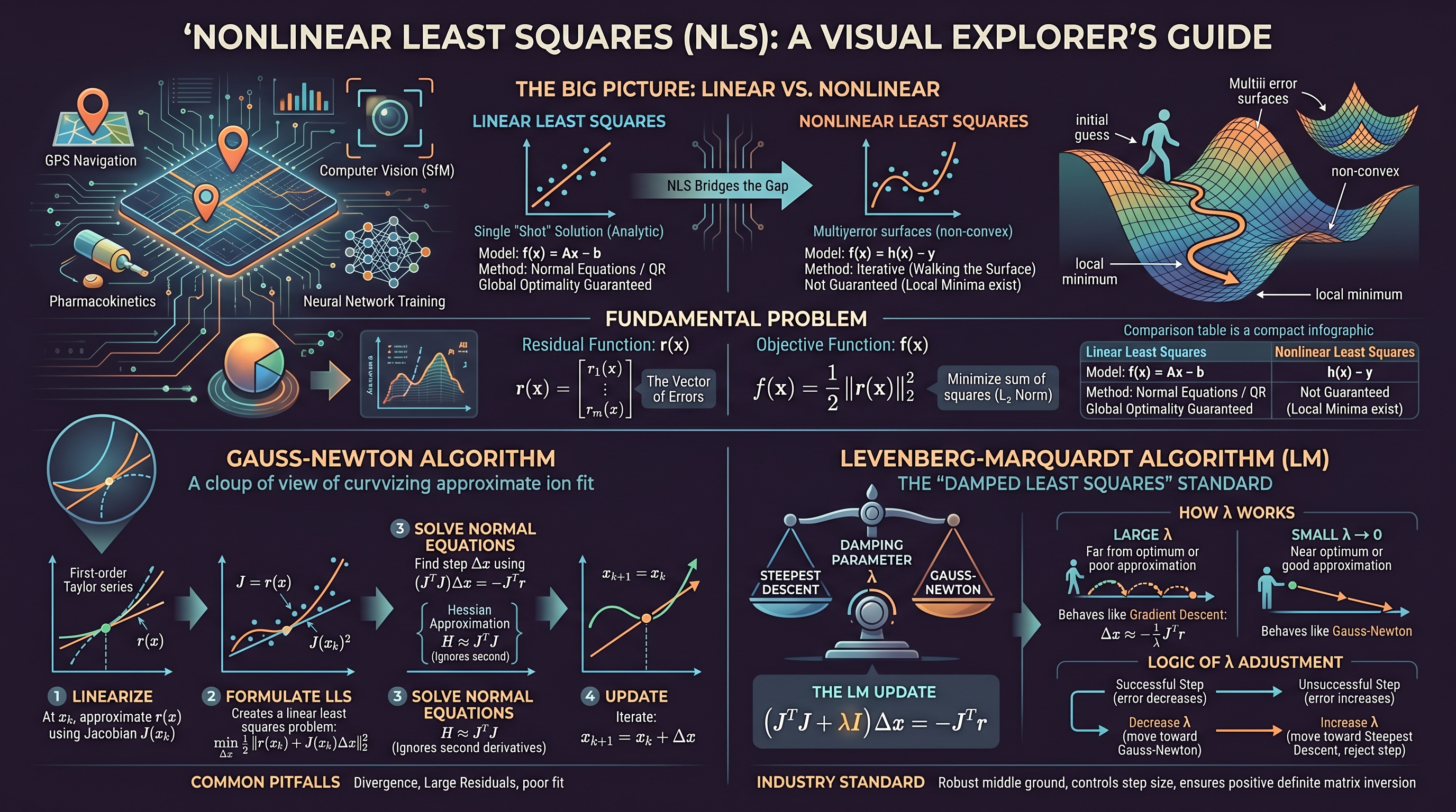
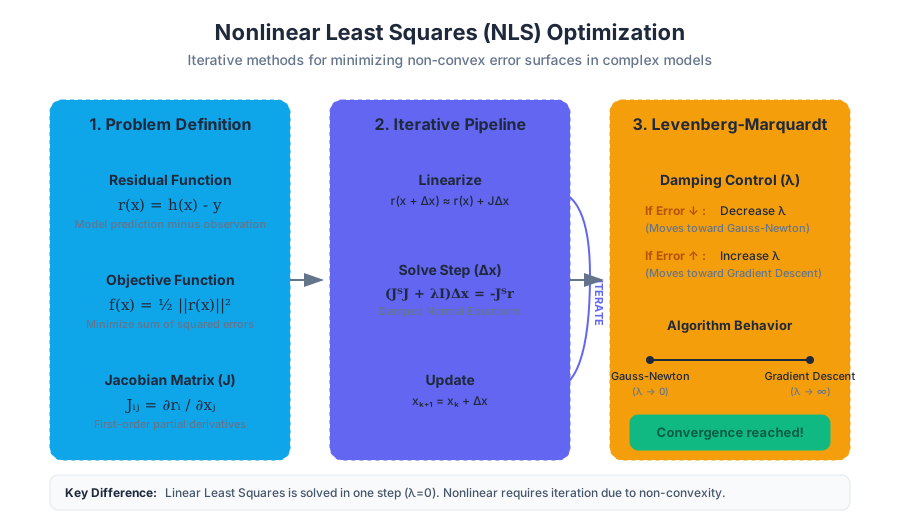
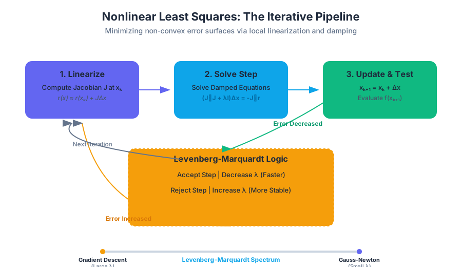
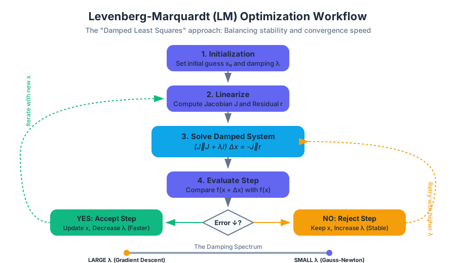
Source Materials
Study Applied Linear Algebra and Least Squares with AI — Free on Lykke
Sign up for free to generate personalized flashcards, quizzes, and study guides from this course. Chat with an AI tutor that knows the material.
Get Started FreeView this course wiki on Lykke · Browse all public course wikis