AP/College Calculus BC
Institution: MIT
42 study materials · 11 sections
This course provides a comprehensive curriculum for AP®/College Calculus BC, covering twelve units of study from foundational limits to advanced infinite series. Students will master differentiation, integration, differential equations, and the calculus of parametric and polar functions. The curriculum is designed to prepare learners for college-level proficiency and the AP Calculus BC exam through structured lessons, practice problems, and detailed exam strategies.
Course Sections
Limits and Continuity
Key concepts: Squeeze Theorem · Intermediate Value Theorem · Discontinuity Classification · Infinite Limits
Foundational concepts of calculus including graphical and algebraic limit estimation and continuity definitions.
Limits and Continuity
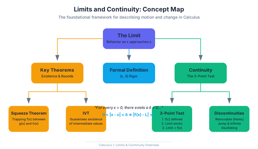
The study of calculus begins not with the derivative or the integral, but with the limit. In the classical Euclidean view, geometry and algebra deal with static objects—points, lines, and equations where variables take on specific, fixed values. Calculus, however, is the mathematics of motion and change. To bridge the gap between the static and the dynamic, we require a rigorous way to describe how a function behaves as it approaches a value, even if it never actually reaches it.
This section explores the formal mechanics of limits, the rigorous definition of continuity, and the foundational theorems—Squeeze and Intermediate Value—that allow us to make certain claims about functions that are otherwise difficult to compute.
The Formal Definition of a Limit
Before we can apply limits to engineering or physics, we must define them with mathematical precision. While the intuitive definition is "the value $L$ that $f(x)$ gets closer to as $x$ gets closer to $c$," this is insufficient for proof-based mathematics.
The formal definition, known as the $(\epsilon, \delta)$-definition of a limit, was popularized by Karl Weierstrass. It removes the "motion" metaphors and replaces them with static inequalities.
Definition: Let $f$ be a function defined on an open interval containing $c$ (except possibly at $c$). We say that: $$\lim_{x \to c} f(x) = L$$ if for every $\epsilon > 0$, there exists a $\delta > 0$ such that if $0 < |x - c| < \delta$, then $|f(x) - L| < \epsilon$.
In plain English: If you pick a tiny distance $\epsilon$ away from the limit $L$, I can find a tiny distance $\delta$ away from $c$ such that every $x$-value in that range maps to a $y$-value within your $\epsilon$-window.
Limit Laws and Algebraic Manipulation
In practice, we rarely use the $(\epsilon, \delta)$ definition for every calculation. Instead, we rely on Limit Laws.
| Law | Formula | Condition |
|---|---|---|
| Sum Law | $\lim (f(x) + g(x)) = \lim f(x) + \lim g(x)$ | Limits must exist |
| Product Law | $\lim (f(x) \cdot g(x)) = \lim f(x) \cdot \lim g(x)$ | Limits must exist |
| Quotient Law | $\lim \frac{f(x)}{g(x)} = \frac{\lim f(x)}{\lim g(x)}$ | $\lim g(x) \neq 0$ |
| Power Law | $\lim [f(x)]^n = [\lim f(x)]^n$ | $n$ is a positive integer |
| Root Law | $\lim \sqrt[n]{f(x)} = \sqrt[n]{\lim f(x)}$ | Valid for $n$ even if $L > 0$ |
The Squeeze Theorem
The Squeeze Theorem (also known as the Sandwich Theorem or the Pinching Theorem) is a technical tool used to find the limit of a function that is "trapped" between two other functions whose limits are known and equal.
The Logic of the Squeeze
Suppose we have three functions such that $g(x) \leq f(x) \leq h(x)$ for all $x$ in an interval around $c$. If the "outer" functions $g(x)$ and $h(x)$ both converge to the same limit $L$ as $x \to c$, then the "inner" function $f(x)$ has no choice but to also converge to $L$.
Theorem: If $g(x) \leq f(x) \leq h(x)$ when $x$ is near $c$ (except possibly at $c$), and $\lim_{x \to c} g(x) = \lim_{x \to c} h(x) = L$, then $\lim_{x \to c} f(x) = L$.
Worked Example: $\lim_{x \to 0} x^2 \sin(\frac{1}{x})$
The function $\sin(\frac{1}{x})$ oscillates infinitely fast as $x$ approaches 0, making the limit difficult to evaluate directly. However, we know the range of the sine function is bounded: $$-1 \leq \sin\left(\frac{1}{x}\right) \leq 1$$ Multiplying the entire inequality by $x^2$ (which is always non-negative): $$-x^2 \leq x^2 \sin\left(\frac{1}{x}\right) \leq x^2$$ As $x \to 0$, both $-x^2 \to 0$ and $x^2 \to 0$. Therefore, by the Squeeze Theorem: $$\lim_{x \to 0} x^2 \sin\left(\frac{1}{x}\right) = 0$$
Continuity: The Three-Point Requirement
In introductory algebra, continuity is often described as "being able to draw the graph without lifting your pencil." In calculus, we require a more rigorous three-part test.
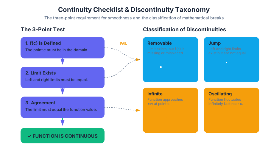
Definition: A function $f(x)$ is continuous at a point $x = c$ if and only if:
- $f(c)$ is defined ($c$ is in the domain).
- $\lim_{x \to c} f(x)$ exists.
- $\lim_{x \to c} f(x) = f(c)$.
If any of these three conditions fail, the function is discontinuous at $c$. Continuity over an interval $[a, b]$ means the function is continuous at every point in $(a, b)$ and possesses one-sided continuity at the endpoints.
Discontinuity Classification
Not all discontinuities are created equal. Engineers and mathematicians categorize them based on how they behave and whether they can be "fixed."
| Type | Description | Graphical Representation | Removable? |
|---|---|---|---|
| Removable | The limit exists, but $f(c)$ is either undefined or different from the limit. | A "hole" in the graph. | Yes (by redefining $f(c)$) |
| Jump | The left-hand limit and right-hand limit both exist but are not equal. | The graph "steps" up or down. | No |
| Infinite | The function approaches $\pm \infty$ as $x$ approaches $c$. | A vertical asymptote. | No |
| Oscillating | The function oscillates infinitely between values as it approaches $c$. | High-frequency "noise" (e.g., $\sin(1/x)$). | No |
The Intermediate Value Theorem (IVT)
The Intermediate Value Theorem is an "existence theorem." It doesn't tell you where a specific value occurs, but it guarantees that the value must exist within a certain interval.
Theorem: If $f$ is continuous on a closed interval $[a, b]$, and $k$ is any number between $f(a)$ and $f(b)$, then there exists at least one number $c$ in $[a, b]$ such that $f(c) = k$.
Practical Application: Root Finding
The IVT is the mathematical basis for the Bisection Method used in computer science to find roots of equations. If a continuous function is negative at $x=a$ and positive at $x=b$, there must be at least one root (where $f(x)=0$) between $a$ and $b$.
# Implementation of the Bisection Method (IVT in action)
def find_root(f, a, b, tol=1e-7):
    """
    Finds a root of function f in the interval [a, b] using the
    Intermediate Value Theorem logic.
    """
    if f(a) * f(b) >= 0:
        raise ValueError("IVT condition not met: f(a) and f(b) must have opposite signs.")

    while (b - a) / 2.0 > tol:
        midpoint = (a + b) / 2.0
        if f(midpoint) == 0:
            return midpoint # Found exact root
        elif f(a) * f(midpoint) < 0:
            b = midpoint # Root is in left half
        else:
            a = midpoint # Root is in right half

    return (a + b) / 2.0

# Example: Finding root of x^3 - x - 2 = 0 between 1 and 2
root = find_root(lambda x: x**3 - x - 2, 1, 2)
print(f"Root found at: {root:.6f}")
Infinite Limits and Asymptotes
When we discuss limits, we often encounter cases where the value of the function grows without bound.
Limits at Infinity ($x \to \infty$)
This describes the end behavior of a function. For rational functions $f(x) = \frac{P(x)}{Q(x)}$, the limit at infinity is determined by the degrees of the polynomials.
- Degree of Numerator < Degree of Denominator: The horizontal asymptote is $y = 0$.
- Degree of Numerator = Degree of Denominator: The horizontal asymptote is the ratio of the leading coefficients.
- Degree of Numerator > Degree of Denominator: There is no horizontal asymptote (the limit is $\pm \infty$).
Infinite Limits ($\lim f(x) = \infty$)
This occurs when the function approaches a vertical asymptote. This usually happens when the denominator of a simplified rational function equals zero.
\text{Example of Vertical Asymptote Behavior:} \\
f(x) = \frac{1}{x-2} \\
\lim_{x \to 2^+} \frac{1}{x-2} = \infty \\
\lim_{x \to 2^-} \frac{1}{x-2} = -\infty
Implementation and Computational Analysis
In modern engineering, limits are often handled symbolically by Computer Algebra Systems (CAS) or numerically when dealing with discrete data.
Symbolic Evaluation with SymPy
For complex limits involving transcendental functions or indeterminate forms, symbolic solvers are preferred over numerical estimation to avoid floating-point errors.
from sympy import Symbol, limit, sin, oo

x = Symbol('x')

# 1. Standard limit
expr1 = (x**2 - 1) / (x - 1)
result1 = limit(expr1, x, 1) # Returns 2

# 2. Limit at infinity
expr2 = (3*x**2 + 5) / (2*x**2 - x)
result2 = limit(expr2, x, oo) # Returns 3/2

# 3. Indeterminate form with Squeeze Theorem context
expr3 = x * sin(1/x)
result3 = limit(expr3, x, 0) # Returns 0

print(f"Limit 1: {result1}, Limit 2: {result2}, Limit 3: {result3}")
Numerical Limit Estimation (Shell/CLI)
Sometimes we need to observe the behavior of a function by sampling points increasingly close to the target value.
# A simple bash loop to observe 1/x behavior as x approaches 0 from the right
for i in {1..6}; do
  val=$(echo "scale=10; 1 / (10^-$i)" | bc)
  printf "x = 10^-%d | f(x) = %s\n" $i $val
done

# Output:
# x = 10^-1 | f(x) = 10
# x = 10^-2 | f(x) = 100
# x = 10^-3 | f(x) = 1000
# ...
Common Pitfalls and Misconceptions
- Confusing "Approaching" with "Being": A limit describes what happens near $c$. The value of $f(c)$ is irrelevant to the existence of the limit.
- Ignoring One-Sided Limits: A limit exists if and only if the left-hand limit equals the right-hand limit. If $\lim_{x \to c^-} f(x) \neq \lim_{x \to c^+} f(x)$, the limit does not exist (DNE).
- The "Infinity is a Number" Fallacy: When we say $\lim f(x) = \infty$, we are describing a behavior (unbounded growth), not stating that the limit is a specific value. In many contexts, an infinite limit is still considered to "not exist" in the finite sense.
- IVT Requirements: The Intermediate Value Theorem only applies if the function is continuous. Applying IVT to a step function or a function with a vertical asymptote will lead to false conclusions.
Summary of Limit Evaluation Strategies
When faced with a limit problem, follow this hierarchy of strategies:
| Step | Strategy | Action |
|---|---|---|
| 1 | Direct Substitution | Plug in $x=c$. If you get a real number, you're done (if $f$ is continuous). |
| 2 | Factoring/Simplification | If you get $0/0$, look for common factors to cancel (Removable Discontinuity). |
| 3 | Rationalization | If square roots are present, multiply by the conjugate. |
| 4 | Special Trig Limits | Use known limits like $\lim_{x \to 0} \frac{\sin x}{x} = 1$. |
| 5 | Squeeze Theorem | Use if the function is bounded by two simpler functions. |
| 6 | L'Hôpital's Rule | (Advanced) Use derivatives for indeterminate forms like $0/0$ or $\infty/\infty$. |
Differentiation: Fundamentals
Key concepts: Power Rule · Product Rule · Quotient Rule · Transcendental Functions
Introduction to the derivative as a limit and basic differentiation rules.
Differentiation: Fundamentals
Overview
Differentiation is the mathematical study of change. While algebra allows us to calculate the average rate of change over a discrete interval, calculus provides the machinery to determine the instantaneous rate of change at a single point. Geometrically, this corresponds to finding the slope of the tangent line to a curve. In the context of physics, if a function represents position over time, its derivative represents velocity; the derivative of velocity, in turn, represents acceleration.
This section moves beyond the intuitive "slope" concept into the rigorous formalisms required for engineering, physics, and advanced data science. We will transition from the computationally expensive Limit Definition to the optimized Differentiation Rules that form the backbone of modern computational mathematics.
The Formal Definition of the Derivative
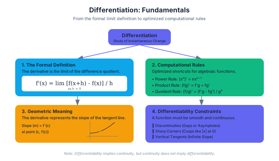
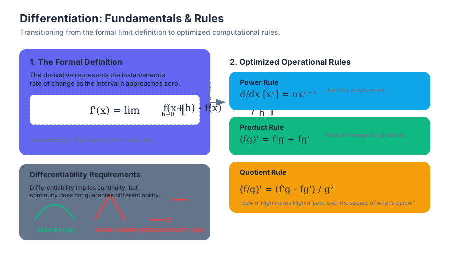
The derivative of a function $f(x)$ at a point $x$, denoted as $f'(x)$ or $\frac{dy}{dx}$, is defined as the limit of the difference quotient as the interval $h$ approaches zero.
Definition: The Derivative For a function $f(x)$, the derivative $f'(x)$ is defined as: $$f'(x) = \lim_{h \to 0} \frac{f(x+h) - f(x)}{h}$$ provided the limit exists. If the limit exists at a point $c$, we say $f$ is differentiable at $c$.
Why the Limit?
In pre-calculus, the slope $m$ is defined as $\frac{\Delta y}{\Delta x}$. However, at a single point, $\Delta x = 0$, leading to the indeterminate form $\frac{0}{0}$. The limit allows us to "zoom in" infinitely close to the point without ever actually dividing by zero, capturing the behavior of the function as it approaches that infinitesimal state.
Differentiability vs. Continuity
A common misconception is that all continuous functions are differentiable. While differentiability implies continuity, the reverse is not true. A function can be continuous but fail to have a derivative at points where the graph has:
- Cusps or Corners: Where the slope changes abruptly (e.g., $f(x) = |x|$ at $x=0$).
- Vertical Tangents: Where the slope approaches infinity (e.g., $f(x) = \sqrt[3]{x}$ at $x=0$).
- Discontinuities: Any break, hole, or asymptote.
| Property | Differentiable Function | Continuous (but not Differentiable) |
|---|---|---|
| Visual Cue | Smooth, unbroken curves | Sharp turns, "kinks," or vertical spikes |
| Limit Existence | $\lim_{h \to 0} \frac{f(x+h)-f(x)}{h}$ exists | Limit of difference quotient diverges |
| Tangent Line | Unique, non-vertical tangent exists | No unique tangent (multiple or vertical) |
| Example | $f(x) = x^2$ | $f(x) = |
The Power Rule
The Power Rule is the primary workhorse for differentiating polynomial functions. It replaces the tedious limit process with a direct algebraic transformation.
Mechanics and Derivation
For any real number $n$, the derivative of $x^n$ is: $$\frac{d}{dx}[x^n] = nx^{n-1}$$
This rule is derived using the Binomial Theorem to expand $(x+h)^n$ in the limit definition. When expanded, all terms except the one containing $nx^{n-1}$ are either cancelled out or remain multiplied by $h$, which vanishes as $h \to 0$.
Application in Engineering
In structural engineering, the Power Rule is used to derive shear force from bending moment equations. If the moment $M(x)$ is a cubic polynomial, the shear force $V(x) = M'(x)$ will be a quadratic polynomial.
# Example 1: Numerical Differentiation (Low-Level Implementation)
# Implementing the symmetric difference quotient for high precision

import numpy as np

def central_difference(f, x, h=1e-5):
    """
    Computes the derivative of f at x using the central difference formula.
    This provides O(h^2) accuracy, better than the forward difference O(h).
    """
    return (f(x + h) - f(x - h)) / (2 * h)

# Define a polynomial function: f(x) = 3x^3 + 2x^2 + 5
f = lambda x: 3*x**3 + 2*x**2 + 5

# Point of interest
x_val = 2.0

# Calculate numerical derivative
derivative = central_difference(f, x_val)

print(f"Numerical derivative at x={x_val}: {derivative:.5f}")
# Analytical check: f'(x) = 9x^2 + 4x -> f'(2) = 9(4) + 4(2) = 36 + 8 = 44
The Product Rule
When two functions are multiplied, the derivative is not simply the product of their derivatives. This is a frequent error for beginners. Instead, we must account for the rate of change of each function while the other remains "momentarily constant."
The Formula
If $h(x) = f(x)g(x)$, then: $$h'(x) = f'(x)g(x) + f(x)g'(x)$$
Derivation Logic
Consider a rectangle with sides $u$ and $v$. The area is $A = uv$. If both sides grow, the change in area $dA$ is composed of the growth of $u$ times $v$, plus the growth of $v$ times $u$, plus the tiny corner where both grow ($du \cdot dv$). In the limit, that tiny corner becomes negligible.
\text{Proof Sketch of Product Rule:}
\begin{aligned}
\frac{d}{dx}[f(x)g(x)] &= \lim_{h \to 0} \frac{f(x+h)g(x+h) - f(x)g(x)}{h} \\
&\text{Add and subtract } f(x+h)g(x) \text{ in the numerator:} \\
&= \lim_{h \to 0} \frac{f(x+h)g(x+h) - f(x+h)g(x) + f(x+h)g(x) - f(x)g(x)}{h} \\
&= \lim_{h \to 0} \left[ f(x+h) \frac{g(x+h)-g(x)}{h} + g(x) \frac{f(x+h)-f(x)}{h} \right] \\
&= f(x)g'(x) + g(x)f'(x)
\end{aligned}
The Quotient Rule
The Quotient Rule is used for functions expressed as ratios. While it can be derived by applying the Product Rule to $f(x) \cdot [g(x)]^{-1}$, the dedicated formula is more efficient for manual calculation.
The Formula
If $h(x) = \frac{f(x)}{g(x)}$, then: $$h'(x) = \frac{f'(x)g(x) - f(x)g'(x)}{[g(x)]^2}$$
Mnemonic: "Low d-High minus High d-Low, over the square of what's below." Where "Low" is the denominator $g(x)$ and "High" is the numerator $f(x)$.
Comparison of Operational Rules
| Rule | Function Form | Derivative Formula | Common Pitfall |
|---|---|---|---|
| Sum/Difference | $f(x) \pm g(x)$ | $f'(x) \pm g'(x)$ | Forgetting to distribute the derivative |
| Product | $f(x)g(x)$ | $f'g + fg'$ | Simply multiplying $f' \cdot g'$ |
| Quotient | $f(x)/g(x)$ | $\frac{f'g - fg'}{g^2}$ | Reversing the numerator order ($fg' - f'g$) |
| Constant Multiple | $cf(x)$ | $cf'(x)$ | Differentiating the constant to zero |
Transcendental Functions
Transcendental functions (trigonometric, exponential, and logarithmic) do not satisfy polynomial equations. Their derivatives are foundational to signal processing, population modeling, and finance.
Trigonometric Derivatives
The derivatives of $\sin(x)$ and $\cos(x)$ are cyclic.
- $\frac{d}{dx}[\sin(x)] = \cos(x)$
- $\frac{d}{dx}[\cos(x)] = -\sin(x)$
These relationships are derived from the angle addition formulas and the fundamental limits $\lim_{\theta \to 0} \frac{\sin \theta}{\theta} = 1$ and $\lim_{\theta \to 0} \frac{\cos \theta - 1}{\theta} = 0$.
Exponential and Logarithmic Derivatives
The natural exponential function $e^x$ is unique in calculus: it is its own derivative.
- $\frac{d}{dx}[e^x] = e^x$
- $\frac{d}{dx}[\ln(x)] = \frac{1}{x}$
The fact that $\frac{d}{dx}[e^x] = e^x$ is actually the defining property of the number $e$. It represents a system where the rate of growth is exactly equal to its current size—the definition of pure exponential growth.
# Example 3: Symbolic Differentiation with SymPy
# Useful for verifying complex analytical derivations in research

import sympy as sp

# Define symbolic variables
x = sp.symbols('x')

# Define a complex transcendental function: f(x) = (e^x * sin(x)) / ln(x)
f_sym = (sp.exp(x) * sp.sin(x)) / sp.log(x)

# Compute the derivative symbolically
f_prime = sp.diff(f_sym, x)

# Simplify the result for readability
f_prime_simplified = sp.simplify(f_prime)

print("Function: ", f_sym)
print("Derivative: ", f_prime_simplified)
Higher-Order Derivatives
A derivative is itself a function, meaning it can be differentiated again.
- First Derivative ($f'$): Velocity, slope, marginal cost.
- Second Derivative ($f''$): Acceleration, concavity, curvature.
- Third Derivative ($f'''$): "Jerk" (the rate of change of acceleration).
Table: Physical Interpretations
| Order | Notation | Physics (Motion) | Geometry | Finance |
|---|---|---|---|---|
| 0 | $s(t)$ | Position | Height of curve | Total Capital |
| 1 | $v(t) = s'(t)$ | Velocity | Slope | Marginal Profit |
| 2 | $a(t) = s''(t)$ | Acceleration | Concavity | Inflation Rate |
| 3 | $j(t) = s'''(t)$ | Jerk | Rate of Curvature | Change in Inflation |
Common Pitfalls and Edge Cases
1. The Constant Rule Confusion
A common mistake is differentiating $e^\pi$ or $2^{10}$ as if they were variables.
- Incorrect: $\frac{d}{dx}[e^\pi] = e^\pi$
- Correct: $\frac{d}{dx}[e^\pi] = 0$ (because $e^\pi$ is a constant).
2. Power Rule with Negative Exponents
When differentiating $f(x) = \frac{1}{x^2}$, rewrite it as $x^{-2}$ first.
- $f'(x) = -2x^{-3} = -\frac{2}{x^3}$.
- Pitfall: Forgetting that subtracting 1 from a negative number makes it "more negative" (e.g., $-2 - 1 = -3$, not $-1$).
3. Logarithmic Domain Restrictions
The derivative of $\ln(x)$ is $\frac{1}{x}$, but this is only defined for $x > 0$. In many engineering contexts, we use $\frac{d}{dx}[\ln|x|] = \frac{1}{x}$, which extends the domain to all $x \neq 0$.
Worked Example: Combining the Rules
Problem: Find the derivative of $f(x) = \frac{x^2 e^x}{\sin(x)}$.
Step 1: Identify the structure. This is a quotient where the numerator is a product. Let $u(x) = x^2 e^x$ and $v(x) = \sin(x)$.
Step 2: Differentiate the numerator ($u$) using the Product Rule. $$u'(x) = \frac{d}{dx}[x^2] \cdot e^x + x^2 \cdot \frac{d}{dx}[e^x]$$ $$u'(x) = 2xe^x + x^2e^x = e^x(2x + x^2)$$
Step 3: Differentiate the denominator ($v$). $$v'(x) = \cos(x)$$
Step 4: Apply the Quotient Rule. $$f'(x) = \frac{u'v - uv'}{v^2}$$ $$f'(x) = \frac{[e^x(2x + x^2)] \cdot \sin(x) - [x^2 e^x] \cdot \cos(x)}{\sin^2(x)}$$
Step 5: Simplify. $$f'(x) = \frac{e^x [ (2x + x^2)\sin(x) - x^2\cos(x) ]}{\sin^2(x)}$$
Advanced Differentiation Techniques
Key concepts: Chain Rule · Implicit Differentiation · Inverse Functions · Higher-Order Derivatives
Techniques for differentiating complex functions, including composite and implicit equations.
Advanced Differentiation Techniques
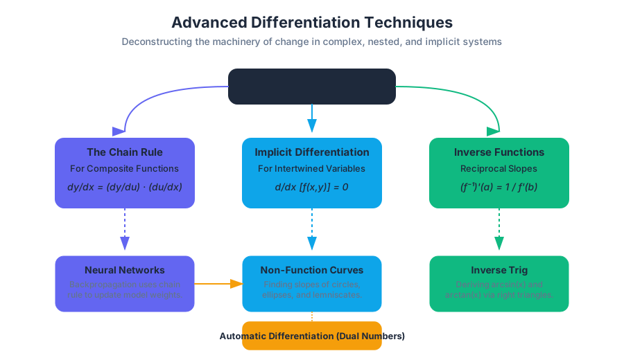
The transition from basic differentiation—applying the power, product, and quotient rules—to advanced techniques marks a pivotal shift in a mathematician's journey. We move from differentiating simple, explicit functions to deconstructing the "machinery of change" in complex systems. This section explores the tools required to handle nested dependencies, non-explicit relations, and the deep layers of change represented by higher-order derivatives.
The Chain Rule: The Engine of Composition
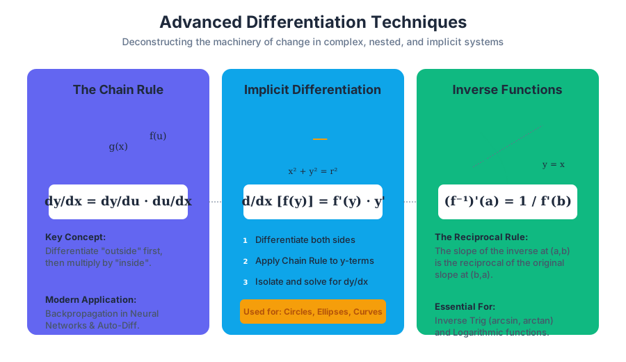
The Chain Rule is arguably the most important rule in all of calculus. It allows us to differentiate composite functions, which are functions where the output of one function becomes the input of another. In the modern era, the Chain Rule is the mathematical backbone of "backpropagation" in neural networks, allowing us to calculate how a change in a single weight affects the total error of a complex model.
Definition and Mechanics
If a variable $y$ depends on $u$, and $u$ in turn depends on $x$, then $y$ depends on $x$ through the intermediate variable $u$. Mathematically, if $y = f(g(x))$, the derivative of $y$ with respect to $x$ is:
$$\frac{dy}{dx} = \frac{dy}{du} \cdot \frac{du}{dx}$$
In Lagrange's notation, this is expressed as: $$(f \circ g)'(x) = f'(g(x)) \cdot g'(x)$$
The "Inside-Outside" Insight: To apply the Chain Rule effectively, always differentiate the "outside" function first (keeping the "inside" function untouched), then multiply by the derivative of the "inside" function.
Notation Comparison
| Notation Type | Expression | Best Use Case |
|---|---|---|
| Leibniz | $\frac{dy}{dx} = \frac{dy}{du} \cdot \frac{du}{dx}$ | Physics, dimensional analysis, and related rates. |
| Lagrange | $f'(g(x)) \cdot g'(x)$ | Theoretical proofs and functional analysis. |
| Operator | $D_x[f(g(x))]$ | Computational logic and symbolic manipulation. |
Implementation in Computational Logic
In modern software engineering, specifically in Machine Learning frameworks like PyTorch or JAX, the Chain Rule is implemented via Automatic Differentiation. Below is a low-level conceptualization of how a "Dual Number" system tracks derivatives using the Chain Rule.
import math

class DualNumber:
    """
    A class representing a value and its derivative (dual part).
    Used to implement automatic differentiation via the Chain Rule.
    """
    def __init__(self, value, derivative=0.0):
        self.v = value
        self.d = derivative

    def __add__(self, other):
        return DualNumber(self.v + other.v, self.d + other.d)

    def __mul__(self, other):
        # Product Rule: (uv)' = u'v + uv'
        return DualNumber(self.v * other.v, self.d * other.v + self.v * other.d)

    def sin(self):
        # Chain Rule: d/dx sin(u) = cos(u) * u'
        return DualNumber(math.sin(self.v), math.cos(self.v) * self.d)

    def __repr__(self):
        return f"Value: {self.v}, Derivative: {self.d}"

# Example: Differentiating sin(x^2) at x=2
# Let f(x) = sin(x^2). f'(x) = cos(x^2) * 2x
x = DualNumber(2.0, 1.0) # x = 2, dx/dx = 1
x_squared = x * x        # u = x^2, du/dx = 2x = 4
result = x_squared.sin() # sin(u), d/dx = cos(u) * du/dx = cos(4) * 4
print(result)
Implicit Differentiation: Handling Hidden Relations
Most introductory calculus problems involve explicit functions, where $y$ is isolated on one side (e.g., $y = x^2 + 1$). However, many mathematical and physical relationships are implicit—the variables are intertwined in a way that is difficult or impossible to solve for $y$ (e.g., $x^2 + y^2 = 25$ or $e^y + \sin(y) = x$).
The Methodology
Implicit differentiation treats $y$ as an implicit function of $x$. When we differentiate a term containing $y$ with respect to $x$, we must apply the Chain Rule, resulting in a $\frac{dy}{dx}$ term.
- Differentiate both sides of the equation with respect to $x$.
- Apply the Chain Rule to every term involving $y$ (multiply by $y'$).
- Collect all terms containing $\frac{dy}{dx}$ on one side.
- Factor out $\frac{dy}{dx}$ and solve.
Comparison: Explicit vs. Implicit
| Feature | Explicit ($y = f(x)$) | Implicit ($F(x, y) = 0$) |
|---|---|---|
| Structure | $y$ is isolated. | $y$ is embedded. |
| Derivation | Direct application of rules. | Requires Chain Rule for $y$ terms. |
| Geometry | Usually represents a single function. | Can represent circles, ellipses, or self-intersecting curves. |
| Difficulty | Generally lower. | Higher; requires algebraic isolation of $y'$. |
Mathematical Derivation of a Circle
Consider the unit circle $x^2 + y^2 = 1$. To find the slope of the tangent line at any point $(x, y)$:
\begin{aligned}
\frac{d}{dx}[x^2 + y^2] &= \frac{d}{dx}[1] \\
2x + 2y \cdot \frac{dy}{dx} &= 0 \\
2y \cdot \frac{dy}{dx} &= -2x \\
\frac{dy}{dx} &= -\frac{x}{y}
\end{aligned}
Derivatives of Inverse Functions
The relationship between a function $f$ and its inverse $f^{-1}$ is a reflection across the line $y=x$. This geometric symmetry implies a specific relationship between their derivatives.
The Inverse Function Theorem
If $f$ is a differentiable function that is one-to-one on an interval, and $f'(f^{-1}(a)) \neq 0$, then the derivative of the inverse function at $a$ is:
$$(f^{-1})'(a) = \frac{1}{f'(f^{-1}(a))}$$
Key Insight: The slope of the inverse function at point $(a, b)$ is the reciprocal of the slope of the original function at point $(b, a)$.
Inverse Trigonometric Functions
Inverse trigonometric functions (like $\arcsin(x)$ or $\arctan(x)$) are essential in integration and physics. Their derivatives are derived using implicit differentiation and right-triangle trigonometry.
Example: Deriving $\frac{d}{dx} \arcsin(x)$
- Let $y = \arcsin(x)$, which implies $\sin(y) = x$.
- Differentiate implicitly: $\cos(y) \cdot \frac{dy}{dx} = 1$.
- Solve for $\frac{dy}{dx} = \frac{1}{\cos(y)}$.
- Use the identity $\cos(y) = \sqrt{1 - \sin^2(y)}$. Since $\sin(y) = x$, then $\cos(y) = \sqrt{1 - x^2}$.
- Result: $\frac{d}{dx} \arcsin(x) = \frac{1}{\sqrt{1 - x^2}}$.
Common Inverse Trig Derivatives
| Function | Derivative | Domain Restriction |
|---|---|---|
| $\arcsin(u)$ | $\frac{u'}{\sqrt{1-u^2}}$ | $\vert u\vert < 1$ |
| $\arccos(u)$ | $-\frac{u'}{\sqrt{1-u^2}}$ | $\vert u\vert < 1$ |
| $\arctan(u)$ | $\frac{u'}{1+u^2}$ | All real $u$ |
| $\text{arcsec}(u)$ | $\frac{u'}{\vert u\vert \sqrt{u^2-1}}$ | $\vert u\vert > 1$ |
Higher-Order Derivatives
A derivative is itself a function, meaning it can be differentiated again. These subsequent derivatives provide deeper insights into the behavior of the original function.
Definitions and Notation
- First Derivative ($f'$ or $\frac{dy}{dx}$): The rate of change (velocity).
- Second Derivative ($f''$ or $\frac{d^2y}{dx^2}$): The rate of change of the rate of change (acceleration/concavity).
- Third Derivative ($f'''$ or $\frac{d^3y}{dx^3}$): Often called "jerk" in physics.
- $n$-th Derivative ($f^{(n)}$): Generalization for any order.
Physical Interpretations
| Order | Name | Physical Meaning |
|---|---|---|
| $s(t)$ | Position | Displacement from origin. |
| $v(t) = s'(t)$ | Velocity | Speed and direction. |
| $a(t) = v'(t) = s''(t)$ | Acceleration | Change in velocity. |
| $j(t) = a'(t) = s'''(t)$ | Jerk | Suddenness of acceleration change. |
Numerical Computation of Higher-Order Derivatives
In systems programming or numerical analysis, we often approximate higher-order derivatives using finite difference methods. This is common in simulations where an analytical derivative is unavailable.
#include <stdio.h>
#include <math.h>

// Function to differentiate: f(x) = x^3
double f(double x) {
    return pow(x, 3);
}

/**
 * Computes the second derivative using the Central Difference Formula:
 * f''(x) ≈ [f(x+h) - 2f(x) + f(x-h)] / h^2
 */
double second_derivative(double (*func)(double), double x, double h) {
    return (func(x + h) - 2 * func(x) + func(x - h)) / (h * h);
}

int main() {
    double x = 2.0;
    double h = 0.001;

    // For f(x) = x^3, f'(x) = 3x^2, f''(x) = 6x.
    // At x=2, f''(2) should be 12.
    double result = second_derivative(f, x, h);

    printf("Analytical f''(2.0) = 12.0\n");
    printf("Numerical f''(2.0)  = %f\n", result);

    return 0;
}
Common Pitfalls and Edge Cases
- Forgetting the Chain Rule in Implicit Differentiation: A common error is differentiating $y^2$ as $2y$ instead of $2y \cdot y'$. Remember that $y$ is a function of $x$.
- Power Rule vs. Chain Rule: Students often misapply the power rule to composite functions, e.g., $\frac{d}{dx} (x^2+1)^3 = 3(x^2+1)^2$ (forgetting to multiply by $2x$).
- Inverse Trig Signs: Confusing the signs of $\arcsin(x)$ and $\arccos(x)$ derivatives. Note that "co-" functions usually have negative derivatives.
- Notation Confusion: $\frac{d^2y}{dx^2}$ is not $(\frac{dy}{dx})^2$. The former is the second derivative; the latter is the square of the first derivative.
Using Symbolic Tools
For complex implicit functions, manual differentiation is prone to error. Engineers often use symbolic math engines to verify results.
# Example using SymPy (Python's symbolic library) via CLI
python3 -c "import sympy as sp; x, y = sp.symbols('x y'); \
           expr = x**2 + y**2 - 25; \
           print('Implicit Derivative dy/dx:', sp.idiff(expr, y, x))"

# Output: Implicit Derivative dy/dx: -x/y
Generalizations: The Multivariable Context
While this section focuses on single-variable calculus, these techniques generalize to multivariable calculus. The Chain Rule becomes a sum of partial derivatives, and implicit differentiation leads to the Implicit Function Theorem, which provides conditions under which an implicit equation locally defines a function. Higher-order derivatives expand into the Hessian Matrix, which is used to find local extrema in high-dimensional spaces.
Contextual Applications of Differentiation
Key concepts: Straight-line Motion · Related Rates · Local Linearity · L'Hôpital's Rule
Applying derivatives to real-world scenarios like motion and related rates.
Contextual Applications of Differentiation
In the abstract realm of calculus, the derivative is defined as the limit of a difference quotient—a purely mathematical construct representing the slope of a tangent line. However, the true power of the derivative is realized when we step out of the Cartesian plane and into the physical world. Contextual Applications of Differentiation bridge the gap between theoretical calculus and empirical reality, providing the mathematical framework to describe motion, optimize systems, and approximate complex behaviors.
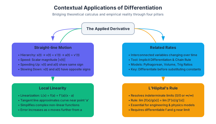
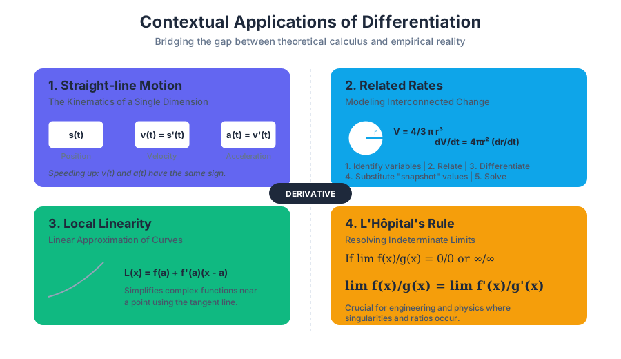
This section explores four pillars of applied differentiation: Straight-line Motion, where we track the kinematics of particles; Related Rates, where we model interconnected variables changing over time; Local Linearity, which allows us to simplify complex curves into manageable lines; and L'Hôpital's Rule, a rigorous tool for resolving indeterminate limits encountered in engineering and physics.
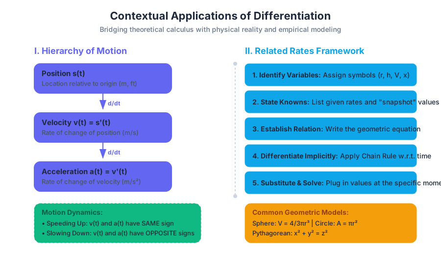
Straight-line Motion: The Kinematics of a Single Dimension
Straight-line motion (or rectilinear motion) is the study of an object moving along a fixed path, typically represented by a coordinate axis. In this context, the derivative is not just a slope; it is a physical rate of change.
The Hierarchy of Motion
We define the state of a particle using three primary functions of time $t$:
- Position $s(t)$: The location of the particle relative to an origin.
- Velocity $v(t) = s'(t)$: The rate of change of position. It indicates both speed and direction.
- Acceleration $a(t) = v'(t) = s''(t)$: The rate of change of velocity.
Definition: Speed vs. Velocity While velocity $v(t)$ is a vector quantity (it can be negative, indicating motion in the "left" or "down" direction), speed is a scalar quantity defined as the absolute value of velocity: $|v(t)|$.
Interpreting Motion Dynamics
To fully understand a particle's behavior, we must analyze the signs of these derivatives.
| Condition | Physical Interpretation |
|---|---|
| $v(t) > 0$ | Particle is moving in the positive direction (Right/Up). |
| $v(t) < 0$ | Particle is moving in the negative direction (Left/Down). |
| $v(t) = 0$ | Particle is momentarily at rest (potential turnaround point). |
| $v(t)$ and $a(t)$ have the same sign | The particle is speeding up. |
| $v(t)$ and $a(t)$ have opposite signs | The particle is slowing down (decelerating). |
Worked Example: Analyzing a Moving Particle
Consider a particle moving along the $x$-axis with position function $s(t) = t^3 - 6t^2 + 9t$ for $t \ge 0$.
- Find Velocity: $v(t) = 3t^2 - 12t + 9 = 3(t-1)(t-3)$.
- Find Acceleration: $a(t) = 6t - 12 = 6(t-2)$.
- Determine Rest Points: The particle is at rest when $v(t) = 0$, which occurs at $t=1$ and $t=3$.
- Intervals of Motion:
- $0 \le t < 1$: $v(t) > 0$ (Moving Right)
- $1 < t < 3$: $v(t) < 0$ (Moving Left)
- $t > 3$: $v(t) > 0$ (Moving Right)
import numpy as np

def analyze_motion(t_vals):
    """
    Calculates position, velocity, and acceleration for a given
    time array using the function s(t) = t^3 - 6t^2 + 9t.
    """
    # Position: s(t) = t^3 - 6t^2 + 9t
    s = t_vals**3 - 6*t_vals**2 + 9*t_vals

    # Velocity: v(t) = 3t^2 - 12t + 9
    v = 3*t_vals**2 - 12*t_vals + 9

    # Acceleration: a(t) = 6t - 12
    a = 6*t_vals - 12

    # Speed: |v(t)|
    speed = np.abs(v)

    return s, v, a, speed

# Example: Analyzing at t = 1.5 seconds
t = np.array([1.5])
pos, vel, acc, spd = analyze_motion(t)

print(f"At t=1.5: Position={pos[0]}, Velocity={vel[0]}, Acceleration={acc[0]}")
# Velocity is negative (-2.25), Acceleration is negative (-3).
# Since signs match, the particle is speeding up in the negative direction.
Related Rates: Modeling Interconnected Change
In many real-world systems, several variables change simultaneously, and their rates of change are linked by a geometric or physical constraint. Related Rates problems use the Chain Rule to find one rate of change in terms of others.
The Procedural Framework
Solving a related rates problem requires a disciplined approach to avoid "premature substitution"—the most common error where students plug in constant values before differentiating.
- Identify Variables: Assign symbols to all changing quantities (e.g., $r$ for radius, $h$ for height, $V$ for volume).
- State the Knowns: Write down the given rates (e.g., $dr/dt = 2$) and the specific "snapshot" moment (e.g., when $r=5$).
- Establish the Relation: Write an equation relating the variables (e.g., $V = \frac{1}{3}\pi r^2 h$).
- Differentiate Implicitly: Differentiate both sides with respect to time $t$.
- Substitute and Solve: Plug in the known values at the specific moment and solve for the unknown rate.
Common Geometric Models
| Shape / Scenario | Primary Equation | Differentiated Form (Example) |
|---|---|---|
| Sphere (Volume) | $V = \frac{4}{3}\pi r^3$ | $\frac{dV}{dt} = 4\pi r^2 \frac{dr}{dt}$ |
| Right Triangle (Pythagorean) | $x^2 + y^2 = z^2$ | $2x\frac{dx}{dt} + 2y\frac{dy}{dt} = 2z\frac{dz}{dt}$ |
| Conical Tank (Volume) | $V = \frac{1}{3}\pi r^2 h$ | Requires substitution of $r$ in terms of $h$ first. |
| Circle (Area) | $A = \pi r^2$ | $\frac{dA}{dt} = 2\pi r \frac{dr}{dt}$ |
Worked Example: The Sliding Ladder
A 10-foot ladder leans against a wall. The bottom of the ladder is pulled away from the wall at a rate of 2 ft/s. How fast is the top of the ladder sliding down the wall when the bottom is 6 feet from the wall?
% Mathematical Derivation for the Sliding Ladder
% Let x = distance from wall to base, y = height of ladder top.
% Constraint: x^2 + y^2 = 10^2 (Pythagorean Theorem)

1. Given: dx/dt = 2, x = 6.
2. Find: dy/dt when x = 6.
3. Find y when x = 6:
   6^2 + y^2 = 100 => 36 + y^2 = 100 => y = 8.
4. Differentiate constraint w.r.t. t:
   d/dt [x^2 + y^2] = d/dt [100]
   2x(dx/dt) + 2y(dy/dt) = 0
5. Substitute:
   2(6)(2) + 2(8)(dy/dt) = 0
   24 + 16(dy/dt) = 0
   dy/dt = -24/16 = -1.5 ft/s.
% The top is sliding down at 1.5 ft/s.
Local Linearity and Linear Approximation
The principle of Local Linearity suggests that if we zoom in far enough on a differentiable curve, the curve looks like a straight line. This "line" is the tangent line at that point. We use this tangent line to approximate the value of the function near the point of tangency.
The Linearization Formula
The linearization $L(x)$ of a function $f$ at a point $a$ is simply the equation of the tangent line:
$$L(x) = f(a) + f'(a)(x - a)$$
Where:
- $f(a)$ is the "starting" value.
- $f'(a)$ is the slope (rate of change).
- $(x - a)$ is the distance from the known point.
Error and Concavity
The accuracy of a linear approximation depends on the concavity of the original function:
- If $f''(x) > 0$ (Concave Up), the tangent line lies below the curve, resulting in an underestimate.
- If $f''(x) < 0$ (Concave Down), the tangent line lies above the curve, resulting in an overestimate.
Practical Usage: Estimating Roots
To estimate $\sqrt{26}$ without a calculator, we use the function $f(x) = \sqrt{x}$ and the known point $a = 25$.
- $f(25) = \sqrt{25} = 5$.
- $f'(x) = \frac{1}{2\sqrt{x}} \implies f'(25) = \frac{1}{10} = 0.1$.
- $L(x) = 5 + 0.1(x - 25)$.
- $L(26) = 5 + 0.1(26 - 25) = 5.1$.
The actual value of $\sqrt{26} \approx 5.099$. Our approximation is remarkably close.
# Using a CLI tool like 'units' or a simple python one-liner for quick linear approx
# Example: f(x) = ln(x), approximate ln(1.1) near a=1
python3 -c "f_a=0; f_prime_a=1; x=1.1; a=1; print(f_a + f_prime_a*(x-a))"
# Output: 0.1
# Actual ln(1.1) is ~0.0953.
L'Hôpital's Rule: Resolving Indeterminacy
In the study of limits, we often encounter forms like $0/0$ or $\infty/\infty$. These are indeterminate forms—they do not have a defined value and could represent any real number or even infinity. L'Hôpital's Rule provides a method to evaluate these limits using derivatives.
The Theorem
If $\lim_{x \to c} f(x) = 0$ and $\lim_{x \to c} g(x) = 0$ (or both are $\pm \infty$), and if $g'(x) \neq 0$ near $c$, then: $$\lim_{x \to c} \frac{f(x)}{g(x)} = \lim_{x \to c} \frac{f'(x)}{g'(x)}$$ provided the limit on the right exists or is $\pm \infty$.
Indeterminate vs. Determinate Forms
It is crucial to distinguish between forms that require L'Hôpital's Rule and those that are already solved.
| Form | Status | Action |
|---|---|---|
| $0/0$ | Indeterminate | Apply L'Hôpital |
| $\infty/\infty$ | Indeterminate | Apply L'Hôpital |
| $0 \cdot \infty$ | Indeterminate | Rewrite as $(f) / (1/g)$ then apply |
| $\infty - \infty$ | Indeterminate | Find common denominator / Rationalize |
| $0/ \infty$ | Determinate | Result is $0$ |
| $\infty / 0$ | Determinate | Result is $\pm \infty$ (Undefined) |
| $1^\infty, 0^0, \infty^0$ | Indeterminate | Use natural logs ($\ln$) to convert to $0 \cdot \infty$ |
Pitfalls and Misconceptions
- The Quotient Rule Trap: L'Hôpital's Rule is not the quotient rule. You differentiate the numerator and denominator separately.
- Premature Application: Do not apply the rule if the limit is not indeterminate. For example, $\lim_{x \to 0} \frac{x+5}{x+1} = 5$. Applying L'Hôpital would incorrectly give $\lim_{x \to 0} \frac{1}{1} = 1$.
- Infinite Loops: Sometimes applying the rule repeatedly leads back to the original form (common with $e^x$ and trig functions). In these cases, algebraic manipulation or the Squeeze Theorem may be required.
Worked Example: Transcendental Limits
Evaluate $\lim_{x \to 0} \frac{e^x - 1 - x}{x^2}$.
- Check Form: $\frac{e^0 - 1 - 0}{0^2} = \frac{0}{0}$. (Indeterminate)
- First Application: Differentiate top and bottom. $$\lim_{x \to 0} \frac{e^x - 1}{2x}$$
- Check Form Again: $\frac{e^0 - 1}{2(0)} = \frac{0}{0}$. (Still Indeterminate)
- Second Application: Differentiate again. $$\lim_{x \to 0} \frac{e^x}{2} = \frac{e^0}{2} = \frac{1}{2}$$
-- Conceptual representation: L'Hôpital as a recursive function
-- This is pseudocode to illustrate the logic flow in a system
WITH RECURSIVE LimitResolver AS (
    SELECT
        numerator_expr AS num,
        denominator_expr AS den,
        0 AS depth
    UNION ALL
    SELECT
        DERIVATIVE(num),
        DERIVATIVE(den),
        depth + 1
    FROM LimitResolver
    WHERE EVAL(num/den) = 'INDETERMINATE' AND depth < 5
)
SELECT EVAL(num/den) FROM LimitResolver WHERE EVAL(num/den) != 'INDETERMINATE';
Summary of Contextual Applications
The transition from "calculating a derivative" to "applying a derivative" represents the shift from being a student of mathematics to being a practitioner of science. Whether we are predicting the point where a particle reverses direction, calculating the rate at which a reservoir empties, or using a tangent line to estimate a complex square root, we are utilizing the derivative as a tool for understanding change.
The concepts of Straight-line Motion and Related Rates emphasize the derivative as a temporal rate ($d/dt$), while Local Linearity and L'Hôpital's Rule leverage the derivative's ability to describe the local geometry of functions. Together, these tools form the backbone of differential modeling in the modern world.
Analytical Applications of Differentiation
Key concepts: Mean Value Theorem · Extreme Value Theorem · First/Second Derivative Tests · Optimization
Using derivatives to analyze function behavior, including extrema and concavity.
Analytical Applications of Differentiation
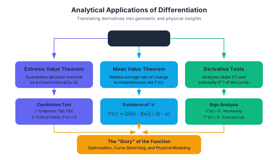
In the preceding study of calculus, the focus was primarily on the mechanics of the derivative: the "how" of differentiation. We mastered the Power Rule, the Chain Rule, and the nuances of transcendental functions. However, the true power of calculus lies in its analytical applications. By examining the derivative of a function, we gain a profound understanding of the function’s geometry, its limits, and its optimal states.
This section serves as the bridge between pure calculation and applied mathematics. We will explore how derivatives allow us to reconstruct the "story" of a function—identifying where it peaks, where it plunges, and how it bends. These tools are the foundation of modern engineering, economic modeling, and physical simulations.
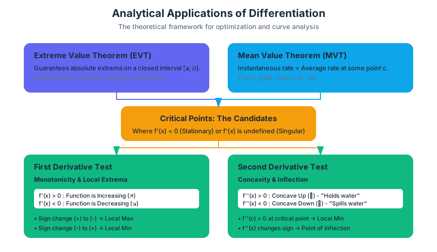
The Extreme Value Theorem (EVT) and Critical Points
Before we can optimize a system, we must guarantee that an optimum actually exists. The Extreme Value Theorem (EVT) provides this theoretical bedrock.
What it is
The EVT states that if a function $f$ is continuous on a closed interval $[a, b]$, then $f$ must attain both an absolute maximum and an absolute minimum on that interval.
The Extreme Value Theorem: Let $f$ be continuous on the closed interval $[a, b]$. There exist numbers $c$ and $d$ in $[a, b]$ such that $f(c) \leq f(x) \leq f(d)$ for all $x$ in $[a, b]$.
Why it matters
In real-world constraints (e.g., a finite budget, a specific range of temperatures, a fixed amount of material), we need to know that a "best" and "worst" case exist. Without the requirement of a closed interval and continuity, a function could head toward infinity or approach a value it never actually reaches, leaving the optimization problem unsolvable.
How it works: The Candidates Test
To find these absolute extrema, we use the Candidates Test. We look at two types of points:
- Critical Points: Values of $x$ where $f'(x) = 0$ or $f'(x)$ is undefined.
- Endpoints: The boundaries $a$ and $b$ of the interval.
| Point Type | Condition | Significance |
|---|---|---|
| Stationary Point | $f'(x) = 0$ | The tangent line is horizontal; potential peak or valley. |
| Singular Point | $f'(x)$ is undefined | A cusp, corner, or vertical tangent; potential extremum. |
| Boundary Point | $x = a$ or $x = b$ | The limits of the domain; often where the absolute max/min resides. |
Low-Level Implementation (Python/SciPy)
In computational science, we often use numerical solvers to find these points when the algebra becomes intractable.
import numpy as np
from scipy.optimize import minimize_scalar

def objective_function(x):
    """The function we want to analyze: f(x) = x**4 - 4x**2 + 3"""
    return x**4 - 4*x**2 + 3

# Defining the closed interval [a, b]
interval = (-2, 2)

# Finding the absolute minimum using a bounded solver
res_min = minimize_scalar(objective_function, bounds=interval, method='bounded')

# Finding the absolute maximum (by minimizing the negative of the function)
res_max = minimize_scalar(lambda x: -objective_function(x), bounds=interval, method='bounded')

print(f"Absolute Minimum at x = {res_min.x:.4f}, f(x) = {res_min.fun:.4f}")
print(f"Absolute Maximum at x = {res_max.x:.4f}, f(x) = {-res_max.fun:.4f}")
The Mean Value Theorem (MVT)
If the EVT guarantees the existence of a destination, the Mean Value Theorem (MVT) describes the relationship between the journey and the average speed.
What it is
The MVT states that for a sufficiently smooth curve, there is at least one point where the instantaneous rate of change (the derivative) equals the average rate of change over an interval.
Mean Value Theorem: If $f$ is continuous on $[a, b]$ and differentiable on $(a, b)$, then there exists at least one point $c$ in $(a, b)$ such that: $$f'(c) = \frac{f(b) - f(a)}{b - a}$$
Mathematical Derivation
The MVT is a generalization of Rolle's Theorem, which covers the specific case where $f(a) = f(b)$.
1. Define a helper function g(x) that represents the vertical distance
   between f(x) and the secant line connecting (a, f(a)) and (b, f(b)).

   g(x) = f(x) - [f(a) + ((f(b) - f(a))/(b - a)) * (x - a)]

2. Note that g(a) = 0 and g(b) = 0.
3. Since f is continuous and differentiable, g is also continuous and differentiable.
4. By Rolle's Theorem, there must be some c in (a, b) such that g'(c) = 0.
5. Differentiate g(x):
   g'(x) = f'(x) - (f(b) - f(a))/(b - a)
6. Set g'(c) = 0:
   0 = f'(c) - (f(b) - f(a))/(b - a)
   f'(c) = (f(b) - f(a))/(b - a)
Concrete Example: Speed Traps
Imagine a car enters a toll road at 12:00 PM and exits 100 miles later at 1:20 PM (1.33 hours). The average speed is $100 / 1.33 \approx 75$ mph. Even if the driver never looks at the speedometer, the MVT proves that at some specific moment $c$ during that trip, the car's instantaneous speed was exactly 75 mph. If the speed limit is 65 mph, the driver was speeding.
The First and Second Derivative Tests
To sketch a function accurately without plotting thousands of points, we analyze the "sign" of its derivatives. This tells us about the function's monotonicity and concavity.
The First Derivative Test: Direction
The first derivative $f'(x)$ tells us if a function is increasing ($f'(x) > 0$) or decreasing ($f'(x) < 0$).
| Sign of $f'(x)$ to the left | Sign of $f'(x)$ to the right | Conclusion at Critical Point $c$ |
|---|---|---|
| Positive (+) | Negative (-) | Relative Maximum |
| Negative (-) | Positive (+) | Relative Minimum |
| Positive (+) | Positive (+) | Neither (Inflection or Shelf) |
| Negative (-) | Negative (-) | Neither (Inflection or Shelf) |
The Second Derivative Test: Concavity
The second derivative $f''(x)$ measures the rate of change of the slope. This is known as concavity.
- If $f''(x) > 0$, the function is concave up (holds water).
- If $f''(x) < 0$, the function is concave down (sheds water).
- An Inflection Point occurs where $f''(x)$ changes sign.
High-Level Usage (C++ Gradient Logic)
In high-performance systems like physics engines, we often use the sign of the derivative to determine the "force" or "direction" of an object's movement toward an equilibrium point.
#include <iostream>
#include <cmath>

// Represents a 1D potential energy function: U(x) = 0.5 * k * x^2
double potential_energy(double x, double k) {
    return 0.5 * k * std::pow(x, 2);
}

// The first derivative (Force): F = -dU/dx = -k * x
double calculate_force(double x, double k) {
    return -k * x;
}

// The second derivative (Stiffness): d^2U/dx^2 = k
double calculate_stiffness(double k) {
    return k;
}

int main() {
    double x = 5.0; // Current position
    double k = 10.0; // Spring constant

    double force = calculate_force(x, k);
    double stiffness = calculate_stiffness(k);

    if (stiffness > 0) {
        std::cout << "System is in a stable equilibrium (Concave Up/Minima)." << std::endl;
    } else if (stiffness < 0) {
        std::cout << "System is in an unstable equilibrium (Concave Down/Maxima)." << std::endl;
    }

    return 0;
}
Applied Optimization
Optimization is the process of finding the "best" solution given a set of constraints. It is the culmination of all the analytical tools discussed above.
The Optimization Workflow
- Identify the Objective Function: What are we trying to maximize or minimize? (e.g., Volume $V$, Cost $C$, Area $A$).
- Identify Constraints: What limits our variables? (e.g., "The surface area must be 500 $cm^2$").
- Substitute: Use the constraint to express the objective function in terms of a single variable.
- Find Critical Points: Differentiate and set to zero.
- Verify: Use the First or Second Derivative Test to ensure the point is the desired extremum.
Worked Example: The Efficient Cylinder
A company wants to design a cylindrical can that holds 1 liter ($1000 cm^3$) of liquid while minimizing the amount of aluminum used (surface area).
Step 1: Objective Function (Surface Area) $$A = 2\pi r^2 + 2\pi rh$$
Step 2: Constraint (Volume) $$V = \pi r^2h = 1000 \implies h = \frac{1000}{\pi r^2}$$
Step 3: Substitute $$A(r) = 2\pi r^2 + 2\pi r \left(\frac{1000}{\pi r^2}\right) = 2\pi r^2 + \frac{2000}{r}$$
Step 4: Differentiate and Solve $$A'(r) = 4\pi r - \frac{2000}{r^2}$$ Set $A'(r) = 0$: $$4\pi r = \frac{2000}{r^2} \implies r^3 = \frac{500}{\pi} \implies r \approx 5.42 \text{ cm}$$
Step 5: Verify $$A''(r) = 4\pi + \frac{4000}{r^3}$$ Since $r > 0$, $A''(r)$ is always positive. The function is concave up, confirming that $r \approx 5.42$ is a minimum.
| Optimization Parameter | Value/Formula |
|---|---|
| Variable | Radius ($r$) |
| Constraint | $V = 1000$ |
| Optimal Radius | $\sqrt[3]{500/\pi} \approx 5.42$ |
| Optimal Height | $2r \approx 10.84$ |
| Ratio ($h/r$) | 2:1 (The most efficient cylinder) |
Common Pitfalls in Analytical Differentiation
Even experienced practitioners fall into specific traps when applying these theorems.
- The "Endpoint" Oversight: When using the EVT, students often find the critical points but forget to check the boundaries $f(a)$ and $f(b)$. In many linear or restricted functions, the maximum occurs at the very edge of the domain.
- The $f''(x) = 0$ Misconception: If the second derivative is zero, the Second Derivative Test is inconclusive. It does not automatically mean there is an inflection point. Consider $f(x) = x^4$; at $x=0$, $f''(0)=0$, but the function has a minimum there, not an inflection point.
- Differentiability Requirements: The MVT requires the function to be differentiable on the open interval. A function with a cusp (like $f(x) = |x|$) on the interval $[-1, 1]$ does not satisfy the MVT, and there is no point where $f'(c) = 0$.
- Implicit vs. Explicit Constraints: In optimization, failing to define the domain based on physical reality (e.g., $r$ must be $> 0$) can lead to mathematically valid but physically impossible solutions.
Summary of Analytical Methods
| Method | Primary Goal | Required Conditions |
|---|---|---|
| EVT / Candidates Test | Finding Absolute Extrema | Continuity on $[a, b]$ |
| Mean Value Theorem | Linking Avg/Inst. Rates | Differentiability on $(a, b)$ |
| First Derivative Test | Finding Local Extrema/Monotonicity | $f$ is continuous at $c$ |
| Second Derivative Test | Finding Local Extrema/Concavity | $f'(c)=0$ and $f''$ exists |
| Optimization | Real-world problem solving | Defined Objective + Constraints |
Integration and Accumulation of Change
Key concepts: Riemann Sums · Fundamental Theorem of Calculus · U-Substitution · Integration by Parts
Introduction to the definite integral, Riemann sums, and the Fundamental Theorem of Calculus.
Integration and Accumulation of Change
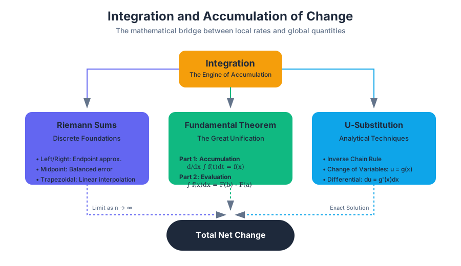
Integration is the mathematical engine of accumulation. While differentiation allows us to zoom in on a single point to find a local rate of change, integration allows us to zoom out, summing those infinitesimal changes to reconstruct the whole. It is the bridge between the local and the global—the process of finding a total quantity when only the rate of its growth is known.
In the context of the AP® Calculus BC curriculum and broader mathematical analysis, this section moves beyond simple "area under a curve" to explore the rigorous foundations of the Definite Integral, the mechanics of the Fundamental Theorem of Calculus, and the sophisticated techniques required to solve complex analytical problems.
Riemann Sums: The Discrete Foundation
Before we can define the integral as a continuous operator, we must understand it as the limit of a discrete sum. A Riemann Sum is an approximation of the area under a curve on a closed interval $[a, b]$ by dividing the area into several geometric shapes (usually rectangles or trapezoids).
The Formal Definition
For a function $f(x)$ defined on $[a, b]$, we partition the interval into $n$ subintervals of width $\Delta x = \frac{b-a}{n}$. The Riemann Sum is defined as:
$$S_n = \sum_{i=1}^{n} f(x_i^*) \Delta x$$
where $x_i^*$ is a sample point in the $i$-th subinterval. As $n \to \infty$, if the function is continuous, this sum converges to the Definite Integral.
Types of Riemann Sums
The choice of the sample point $x_i^*$ determines the type of sum and the nature of the approximation error.
| Method | Sample Point ($x_i^*$) | Characteristic | Error Behavior |
|---|---|---|---|
| Left Riemann Sum | Left endpoint of subinterval | Underestimates increasing functions | $O(\Delta x)$ |
| Right Riemann Sum | Right endpoint of subinterval | Overestimates increasing functions | $O(\Delta x)$ |
| Midpoint Rule | Center of subinterval | Highly accurate; balances error | $O(\Delta x^2)$ |
| Trapezoidal Rule | Average of endpoints | Uses trapezoids instead of rectangles | $O(\Delta x^2)$ |
The Trapezoidal Rule Derivation
The Trapezoidal Rule is often more efficient than endpoint sums because it accounts for the slope of the function. The area of a single trapezoid is $\frac{1}{2}(f(x_{i-1}) + f(x_i))\Delta x$. Summing these across the interval yields the composite Trapezoidal Rule:
$$T_n = \frac{\Delta x}{2} \left[ f(x_0) + 2f(x_1) + 2f(x_2) + \dots + 2f(x_{n-1}) + f(x_n) \right]$$
Implementation: Numerical Integration
In engineering contexts, we rarely integrate symbolic functions; we integrate discrete data points. Below is a robust Python implementation of the Trapezoidal and Simpson's rules for numerical integration.
import numpy as np

def numerical_integrate(f, a, b, n, method='trapezoidal'):
    """
    Performs numerical integration on a function f from a to b.

    Parameters:
    f: callable function
    a, b: bounds of integration
    n: number of subintervals
    method: 'trapezoidal' or 'midpoint'
    """
    if n <= 0:
        raise ValueError("Number of intervals n must be positive.")

    x = np.linspace(a, b, n + 1)
    dx = (b - a) / n

    if method == 'trapezoidal':
        # T = (dx/2) * (f(x0) + 2f(x1) + ... + f(xn))
        y = f(x)
        return (dx / 2) * (y[0] + 2 * np.sum(y[1:-1]) + y[-1])

    elif method == 'midpoint':
        # M = dx * sum(f(midpoints))
        midpoints = x[:-1] + dx / 2
        return dx * np.sum(f(midpoints))

    else:
        raise NotImplementedError(f"Method {method} not supported.")

# Example: Integrate x^2 from 0 to 1 (Expected: 1/3)
func = lambda x: x**2
result = numerical_integrate(func, 0, 1, 1000, method='trapezoidal')
print(f"Result: {result:.6f}")
The Fundamental Theorem of Calculus (FTC)
The Fundamental Theorem of Calculus is the "Great Unification" of mathematics. It establishes that differentiation and integration are inverse processes, effectively linking the geometry of area to the algebra of rates.
FTC Part 1: The Accumulation Function
The first part of the theorem describes the derivative of an accumulation function. If $f$ is continuous on $[a, b]$, then the function $g(x)$ defined by:
$$g(x) = \int_{a}^{x} f(t) , dt$$
is continuous on $[a, b]$, differentiable on $(a, b)$, and its derivative is:
$$g'(x) = f(x)$$
Insight: This tells us that the rate at which area accumulates under $f(t)$ at the point $x$ is exactly the value of the function $f(x)$.
FTC Part 2: Evaluation of Definite Integrals
The second part provides the practical tool for calculating integrals without limits of sums. If $F$ is any antiderivative of $f$ (meaning $F' = f$), then:
$$\int_{a}^{b} f(x) , dx = F(b) - F(a)$$
Comparison of FTC Applications
| Feature | FTC Part 1 (Accumulation) | FTC Part 2 (Evaluation) |
|---|---|---|
| Primary Goal | To find the derivative of an integral | To find the numeric value of an integral |
| Input | A function defined as an integral | A definite integral with fixed bounds |
| Output | A function ($f(x)$) | A scalar value ($C$) |
| Key Use Case | Solving differential equations | Finding area, volume, or net change |
Integration Techniques: U-Substitution
U-Substitution is the integration equivalent of the Chain Rule. It is used to simplify an integral by changing the variable of integration to a new variable $u$, which represents a "nested" function within the integrand.
The Mechanics
If we have an integral of the form $\int f(g(x))g'(x) , dx$, we let $u = g(x)$. Then, the differential $du = g'(x) , dx$. The integral transforms into:
$$\int f(u) , du$$
Worked Example: Definite Integral with U-Sub
Evaluate $\int_{0}^{\sqrt{\pi}} x \sin(x^2) , dx$.
- Identify $u$: Let $u = x^2$.
- Find $du$: $du = 2x , dx \implies \frac{1}{2}du = x , dx$.
- Change Bounds:
- Lower: If $x = 0$, $u = 0^2 = 0$.
- Upper: If $x = \sqrt{\pi}$, $u = (\sqrt{\pi})^2 = \pi$.
- Substitute and Integrate: $$\frac{1}{2} \int_{0}^{\pi} \sin(u) , du = \frac{1}{2} [-\cos(u)]_{0}^{\pi}$$ $$\frac{1}{2} [-\cos(\pi) - (-\cos(0))] = \frac{1}{2} [1 + 1] = 1$$
\begin{aligned}
\text{Step 1: } & u = g(x) \\
\text{Step 2: } & \frac{du}{dx} = g'(x) \implies du = g'(x)dx \\
\text{Step 3: } & \int f(g(x))g'(x)dx = \int f(u)du \\
\text{Step 4: } & \text{Integrate } F(u) + C \\
\text{Step 5: } & \text{Back-substitute } F(g(x)) + C
\end{aligned}
Integration by Parts (IBP)
Where U-substitution reverses the Chain Rule, Integration by Parts reverses the Product Rule. It is the primary tool for integrating the product of two functions, especially when one function simplifies upon differentiation and the other is easily integrable.
The Derivation
Starting with the Product Rule: $$\frac{d}{dx}[uv] = u\frac{dv}{dx} + v\frac{du}{dx}$$ Integrating both sides and rearranging gives the IBP formula:
$$\int u , dv = uv - \int v , du$$
Choosing $u$: The LIATE Rule
The success of IBP depends entirely on the choice of $u$. We use the LIATE mnemonic to prioritize which function should be assigned to $u$:
| Priority | Category | Examples |
|---|---|---|
| L | Logarithmic Functions | $\ln(x), \log_2(x)$ |
| I | Inverse Trigonometric | $\arctan(x), \arcsin(x)$ |
| A | Algebraic Functions | $x^2, 3x, \sqrt{x}$ |
| T | Trigonometric Functions | $\sin(x), \cos(x)$ |
| E | Exponential Functions | $e^x, 2^x$ |
Tabular Integration (The DI Method)
For integrals requiring multiple rounds of IBP (like $\int x^3 e^x , dx$), the "DI Method" is a high-speed alternative to the standard formula. You create two columns: D (to be differentiated) and I (to be integrated).
- List $u$ and its successive derivatives in the D column until you reach 0.
- List $dv$ and its successive integrals in the I column.
- Assign alternating signs (+, -, +, -) to the rows.
- Multiply diagonally.
Real-World Context: Signal Processing
In electrical engineering, integration by parts is used to compute the Fourier Transform, which decomposes signals into their constituent frequencies.
#include <iostream>
#include <cmath>
#include <vector>

// High-level representation of a Fourier-like accumulation
// using a simple numerical integration approach.
double compute_integral_step(double (*func)(double), double t, double freq) {
    // In actual signal processing, we integrate f(t) * exp(-i * omega * t)
    // This snippet demonstrates the kernel of such a calculation.
    return func(t) * std::cos(2.0 * M_PI * freq * t);
}

int main() {
    auto signal = [](double t) { return std::exp(-t); }; // Example signal
    double frequency = 1.0;
    double lower_bound = 0.0;
    double upper_bound = 5.0;
    int steps = 1000;
    double dt = (upper_bound - lower_bound) / steps;

    double total_accumulation = 0.0;
    for(int i = 0; i < steps; ++i) {
        double t = lower_bound + i * dt;
        total_accumulation += compute_integral_step(signal, t, frequency) * dt;
    }

    std::cout << "Accumulated Signal Component: " << total_accumulation << std::endl;
    return 0;
}
Advanced Accumulation: Improper Integrals
In many physics and statistics applications, we encounter integrals where the interval of integration is infinite or the integrand has a vertical asymptote. These are Improper Integrals.
Type 1: Infinite Intervals
$$\int_{a}^{\infty} f(x) , dx = \lim_{t \to \infty} \int_{a}^{t} f(x) , dx$$ If the limit exists as a finite number, the integral converges. If not, it diverges.
Type 2: Discontinuous Integrands
If $f(x)$ has an infinite discontinuity at $b$: $$\int_{a}^{b} f(x) , dx = \lim_{t \to b^-} \int_{a}^{t} f(x) , dx$$
The p-Series Test for Integrals
A critical shortcut for convergence: $$\int_{1}^{\infty} \frac{1}{x^p} , dx \text{ converges if } p > 1, \text{ and diverges if } p \leq 1.$$
Common Pitfalls and Misconceptions
- Forgetting the Constant of Integration ($+C$): When performing indefinite integration, the result is a family of functions. Omitting $+C$ is a failure to acknowledge the vertical shift.
- Ignoring Discontinuities: Applying FTC Part 2 to a function with a vertical asymptote in the middle of the interval (e.g., $\int_{-1}^{1} \frac{1}{x^2} , dx$) will yield a nonsense result. You must split the integral and use limits.
- Incorrect U-Substitution Bounds: A common error is substituting $u$ but keeping the $x$-limits. Always transform the bounds or back-substitute before evaluating.
- Misidentifying $u$ in IBP: Choosing an exponential for $u$ and a polynomial for $dv$ usually makes the integral more complicated rather than less. Stick to LIATE.
Differential Equations
Key concepts: Slope Fields · Euler's Method · Separation of Variables · Logistic Growth
Solving and modeling equations that involve derivatives.
Differential Equations
Differential equations (DEs) represent the pinnacle of the calculus sequence, serving as the bridge between abstract mathematical theory and the physical reality of a changing world. While standard calculus focuses on finding the rate of change of a known function, differential equations invert this relationship: we are given the rate of change (the derivative) and must reconstruct the original function.
In the words of the physicist Richard Feynman, "The laws of nature are expressed as differential equations." From the cooling of a cup of coffee to the vibrations of a bridge or the spread of a viral pathogen, differential equations provide the rigorous framework necessary to model, predict, and control dynamic systems.
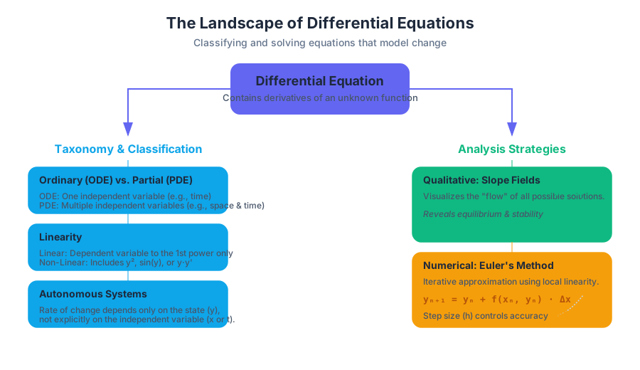
The Fundamental Landscape of Differential Equations
A differential equation is any equation that contains one or more derivatives of an unknown function. The order of the equation is determined by the highest derivative present. In introductory contexts, we focus primarily on First-Order Ordinary Differential Equations (ODEs), which take the general form:
$$\frac{dy}{dx} = f(x, y)$$
Where $y$ is an unknown function of $x$. Solving such an equation means finding a function $y = \phi(x)$ that satisfies the relationship for all $x$ in a given interval.
Classification and Terminology
To navigate this field, one must understand the taxonomy of DEs:
| Term | Definition | Example |
|---|---|---|
| Ordinary (ODE) | Contains derivatives with respect to only one independent variable. | $\frac{dy}{dx} + 5y = e^x$ |
| Partial (PDE) | Contains derivatives with respect to multiple independent variables. | $\frac{\partial^2 u}{\partial t^2} = c^2 \frac{\partial^2 u}{\partial x^2}$ |
| Linear | The dependent variable and its derivatives appear only to the first power. | $y'' + 3y' + 2y = 0$ |
| Non-Linear | The dependent variable or its derivatives are multiplied together or involve non-linear functions. | $\frac{dy}{dx} = y^2 + \sin(y)$ |
| Autonomous | The rate of change depends only on the dependent variable, not the independent one. | $\frac{dy}{dt} = ky(1 - \frac{y}{K})$ |
Slope Fields: Visualizing the Derivative
When an analytical solution to a differential equation is difficult or impossible to find, we turn to qualitative analysis. Slope Fields (or direction fields) are the primary tool for this.
What it is
A slope field is a graphical representation of the slopes of all possible solution curves for a first-order DE. At every point $(x, y)$ in the plane, we draw a small line segment with a slope equal to $f(x, y)$.
Why it matters
Slope fields allow us to visualize the "flow" of a system. Even without solving the equation, we can determine the long-term behavior (asymptotic behavior) of a solution and identify equilibrium points where $dy/dx = 0$.
Construction and Interpretation
To construct a slope field for $\frac{dy}{dx} = x - y$:
- Select a grid of points (e.g., integers from -3 to 3).
- Calculate the value of $x - y$ at each point.
- Draw a short segment with that calculated slope at that point.
Theorem: Existence and Uniqueness If $f(x, y)$ and $\frac{\partial f}{\partial y}$ are continuous in a region containing $(x_0, y_0)$, then there exists a unique solution curve passing through that point. This ensures that solution curves in a slope field never cross.
Euler's Method: Numerical Approximation
Not every differential equation can be solved with pen and paper. In engineering and computational science, we often use Euler's Method, the most fundamental numerical technique for approximating the solution to an Initial Value Problem (IVP).
Mechanics of the Algorithm
Euler's Method relies on the concept of local linearity. If we know a starting point $(x_0, y_0)$ and the slope at that point $f(x_0, y_0)$, we can move a small distance $\Delta x$ (the step size) along the tangent line to find an approximate next point $(x_1, y_1)$.
The iterative formulas are:
- $x_{n+1} = x_n + \Delta x$
- $y_{n+1} = y_n + f(x_n, y_n) \cdot \Delta x$
Worked Example
Approximate $y(1.2)$ for $\frac{dy}{dx} = x + y$ with initial condition $y(1) = 0$ and step size $\Delta x = 0.1$.
- Step 1: $x_0 = 1, y_0 = 0$. Slope $m = 1+0 = 1$. $y_1 = 0 + (1)(0.1) = 0.1$. New point: $(1.1, 0.1)$.
- Step 2: $x_1 = 1.1, y_1 = 0.1$. Slope $m = 1.1 + 0.1 = 1.2$. $y_2 = 0.1 + (1.2)(0.1) = 0.22$. New point: $(1.2, 0.22)$.
The approximation for $y(1.2)$ is $0.22$.
Implementation in Python
The following implementation demonstrates Euler's method applied to a non-linear system, comparing the numerical result against an analytical baseline.
import numpy as np

def euler_method(f, x0, y0, h, steps):
    """
    Computes the numerical approximation of an ODE using Euler's Method.

    Args:
        f: The derivative function dy/dx = f(x, y)
        x0, y0: Initial conditions
        h: Step size
        steps: Number of iterations
    """
    x_values = np.zeros(steps + 1)
    y_values = np.zeros(steps + 1)

    x_values[0], y_values[0] = x0, y0

    for i in range(steps):
        # The core Euler update logic
        slope = f(x_values[i], y_values[i])
        y_values[i+1] = y_values[i] + slope * h
        x_values[i+1] = x_values[i] + h

    return x_values, y_values

# Example: dy/dx = y (Exponential growth)
# Analytical solution: y = e^x
f_prime = lambda x, y: y
x_pts, y_pts = euler_method(f_prime, 0, 1, 0.1, 10)

print(f"Approximation at x=1.0: {y_pts[-1]:.4f}")
print(f"Exact value (e^1): {np.exp(1):.4f}")
Error Analysis
Euler's method is a first-order method, meaning the local truncation error is $O(h^2)$ and the global truncation error is $O(h)$.
| Factor | Effect on Accuracy | Trade-off |
|---|---|---|
| Step Size ($h$) | Smaller $h$ reduces truncation error. | Increases computational cost and round-off error. |
| Curvature ($y''$) | High curvature increases error (linear approximation fails). | Requires adaptive step-size methods (like Runge-Kutta). |
| Interval Length | Errors accumulate over longer intervals. | May require more sophisticated "multi-step" methods. |
Separation of Variables: Analytical Precision
Separation of Variables is the primary algebraic technique for solving first-order DEs. It is applicable when the derivative can be factored into a product of a function of $x$ and a function of $y$.
The Derivation
Given $\frac{dy}{dx} = g(x)h(y)$, we assume $h(y) \neq 0$ and rewrite the equation:
\begin{aligned}
\frac{1}{h(y)} dy &= g(x) dx \\
\int \frac{1}{h(y)} dy &= \int g(x) dx \\
H(y) &= G(x) + C
\end{aligned}
This yields an implicit solution. If possible, we solve for $y$ to get the explicit solution.
Worked Example: The Particular Solution
Solve $\frac{dy}{dx} = \frac{2x}{y}$ with the initial condition $y(0) = -3$.
- Separate: $y , dy = 2x , dx$
- Integrate: $\int y , dy = \int 2x , dx \implies \frac{1}{2}y^2 = x^2 + C$
- Apply Initial Condition: $\frac{1}{2}(-3)^2 = (0)^2 + C \implies C = 4.5$
- Solve for y: $\frac{1}{2}y^2 = x^2 + 4.5 \implies y^2 = 2x^2 + 9 \implies y = \pm\sqrt{2x^2 + 9}$
- Select Branch: Since $y(0) = -3$, we must choose the negative root: $y = -\sqrt{2x^2 + 9}$.
Common Pitfalls
- The Constant of Integration ($C$): Forgetting $C$ is the most common error. $C$ must be introduced the moment the integral is performed, not added at the end.
- Absolute Values: When integrating $1/y$, the result is $\ln|y|$. Removing the natural log requires $e^{\ln|y|} = e^{f(x)+C}$, which becomes $|y| = e^C e^{f(x)}$. This is often simplified to $y = Ae^{f(x)}$, where $A = \pm e^C$.
- Singular Solutions: Dividing by $h(y)$ assumes $h(y) \neq 0$. Values of $y$ that make $h(y) = 0$ are constant solutions that might be missed by the separation process.
Growth Models: Exponential vs. Logistic
Differential equations are the standard for modeling population dynamics. We generally distinguish between "unconstrained" and "constrained" growth.
Exponential Growth
The simplest model assumes the rate of growth is proportional to the current population: $$\frac{dP}{dt} = kP$$ Using separation of variables, this yields the familiar $P(t) = P_0 e^{kt}$. While accurate for short periods, it fails for long-term modeling because it ignores resource limits.
Logistic Growth
The Logistic Model introduces a Carrying Capacity ($K$), the maximum population the environment can sustain. The rate of growth is proportional to both the current population and the remaining "room" for growth.
$$\frac{dP}{dt} = kP \left( 1 - \frac{P}{K} \right)$$
Solving the Logistic Equation
This equation is solved using separation of variables and partial fraction decomposition:
\begin{aligned}
\int \frac{dP}{P(1 - P/K)} &= \int k \, dt \\
\int \left( \frac{1}{P} + \frac{1/K}{1 - P/K} \right) dP &= kt + C \\
\ln|P| - \ln|1 - P/K| &= kt + C \\
\ln \left| \frac{P}{1 - P/K} \right| &= kt + C
\end{aligned}
Solving for $P$ gives the general solution: $$P(t) = \frac{K}{1 + Ae^{-kt}}$$ where $A = \frac{K - P_0}{P_0}$.
Key Features of Logistic Growth
| Feature | Mathematical Condition | Physical Meaning |
|---|---|---|
| Max Growth Rate | $P = K/2$ | The population grows fastest when it is half-full. |
| Inflection Point | $\frac{d^2P}{dt^2} = 0$ | The point where growth shifts from accelerating to decelerating. |
| Asymptote | $\lim_{t \to \infty} P(t) = K$ | The population stabilizes at the carrying capacity. |
| Equilibrium | $P=0$ or $P=K$ | Points where the population does not change. |
Advanced Tooling: Symbolic Computation
In professional practice, we often use symbolic engines to verify solutions or handle complex integration. Below is a demonstration of solving a differential equation using SymPy, a Python library for symbolic mathematics.
from sympy import symbols, Function, Eq, dsolve, exp

# Define symbols
t = symbols('t')
P = Function('P')
k, K = symbols('k K', real=True, positive=True)

# Define the Logistic Differential Equation
# dP/dt = k * P * (1 - P/K)
logistic_eq = Eq(P(t).diff(t), k * P(t) * (1 - P(t)/K))

# Solve the equation symbolically
solution = dsolve(logistic_eq, P(t))

print("General Solution for Logistic Growth:")
print(solution)
For engineers working in the field, a quick CLI check using a tool like gnuplot can visualize a slope field instantly:
# Gnuplot command to visualize a slope field for dy/dx = sin(x)*cos(y)
gnuplot -e "set terminal png; set output 'slopefield.png'; \
            set xrange [-3:3]; set yrange [-3:3]; \
            plot '++' u 1:2:(0.1):(0.1*(sin($1)*cos($2))) \
            with vectors head filled lt 2 title 'dy/dx = sin(x)cos(y)'"
Summary of Methods
| Method | Best Used When... | Pros | Cons |
|---|---|---|---|
| Slope Fields | Qualitative behavior is needed. | No integration required; handles non-linearities. | No exact numerical values. |
| Euler's Method | No analytical solution exists. | Easy to program; works on almost any DE. | Accumulates error; requires small steps. |
| Separation of Variables | Equation is of the form $f(y)dy = g(x)dx$. | Provides exact, analytical functions. | Only works for a small subset of DEs. |
| Growth Models | Modeling biological or social systems. | Highly predictive for real-world data. | Requires estimating parameters like $k$ and $K$. |
Applications of Integration
Key concepts: Average Value · Net Change · Area Between Curves · Volume by Cross Sections
Using integrals to find average values, areas between curves, and volumes.
Applications of Integration: From Accumulation to Geometry
The definite integral is often introduced as the "area under a curve," but this geometric interpretation is merely the surface of a much deeper mathematical well. In the context of advanced calculus and engineering, integration is the fundamental tool for accumulation. It allows us to reconstruct global quantities from local, infinitesimal rates of change. Whether we are determining the average temperature of a cooling engine, the total displacement of a particle under varying acceleration, or the precise volume of a complex mechanical part, we rely on the same underlying principle: the limit of a Riemann sum.
Average Value of a Function
In discrete mathematics, the average of a set of numbers is the sum divided by the count. However, for a continuous function $f(x)$ on an interval $[a, b]$, there are infinitely many points. We cannot sum them individually. Instead, we use the integral to "smooth out" the function into a rectangle with the same area.
1. Definition and Mathematical Notation
The Average Value of a continuous function $f$ over the interval $[a, b]$ is defined as:
Definition: $f_{avg} = \frac{1}{b-a} \int_{a}^{b} f(x) , dx$
This concept is inextricably linked to the Mean Value Theorem for Integrals, which guarantees that for a continuous function, there exists at least one point $c$ in $[a, b]$ such that $f(c) = f_{avg}$.
2. Why It Matters
In thermodynamics, we use average values to find the mean kinetic energy of particles. In electrical engineering, the Root Mean Square (RMS) voltage—a variation of the average value—is used to define the effective voltage of an alternating current (AC).
3. Comparison: Discrete vs. Continuous Average
| Feature | Discrete Average (Arithmetic Mean) | Continuous Average (Integral Mean) |
|---|---|---|
| Input Type | Finite set of points ${x_1, x_2, ... x_n}$ | Continuous function $f(x)$ on $[a, b]$ |
| Summation Method | $\sum_{i=1}^{n} x_i$ | $\int_{a}^{b} f(x) , dx$ |
| Normalization | Divide by $n$ (count) | Divide by $b-a$ (interval length) |
| Physical Analogy | Average height of students in a class | Average height of a mountain range |
4. Implementation Example: Numerical Integration
In practice, especially with sensor data, we often compute the average value using numerical methods like the Trapezoidal Rule.
import numpy as np

def calculate_average_value(func, a, b, n=1000):
    """
    Computes the average value of a function over [a, b]
    using the Composite Trapezoidal Rule.
    """
    x = np.linspace(a, b, n)
    y = func(x)

    # Definite integral via trapezoidal integration
    integral = np.trapz(y, x)

    # Average value formula: (1 / (b - a)) * integral
    avg_val = (1 / (b - a)) * integral
    return avg_val

# Example: Average value of sin(x) from 0 to Pi
# Analytical result: (1/Pi) * [-cos(x)]_0^Pi = 2/Pi ≈ 0.6366
f = lambda x: np.sin(x)
print(f"Calculated Average: {calculate_average_value(f, 0, np.pi)}")
Net Change and Accumulation
The Net Change Theorem is a direct application of the Fundamental Theorem of Calculus. It states that the integral of a rate of change is the net change in the original quantity.
1. The Mechanics of Accumulation
If $F'(x)$ represents the rate at which a quantity is changing, then: $$\int_{a}^{b} F'(x) , dx = F(b) - F(a)$$
This is vital in physics when distinguishing between displacement and total distance traveled.
- Displacement: $\int_{t_1}^{t_2} v(t) , dt$ (The net change in position).
- Total Distance: $\int_{t_1}^{t_2} |v(t)| , dt$ (The accumulation of all movement, regardless of direction).
2. Derivation of the Accumulation Function
We can define an accumulation function $S(x)$ that represents the quantity gathered from a starting point $a$ to a variable point $x$:
S(x) = \int_{a}^{x} f(t) \, dt
Where:
- $f(t)$ is the rate of change (e.g., liters per second).
- $S(x)$ is the total amount accumulated (e.g., total liters).
3. Common Pitfalls: Signs and Direction
A common error is neglecting the sign of the function. In a net change problem involving a tank being filled and drained simultaneously, the rate function $R(t) = Inflow(t) - Outflow(t)$ can be negative. The integral will correctly reflect the "net" volume, but if you are asked for the "total volume processed," you must integrate the absolute value.
Area Between Curves
Calculating the area between two curves $f(x)$ and $g(x)$ is the process of integrating the vertical (or horizontal) distance between them over a specific interval.
1. Vertical Slices ($dx$) vs. Horizontal Slices ($dy$)
The choice of orientation depends on the geometry of the functions.
Theorem: If $f(x) \geq g(x)$ for all $x$ in $[a, b]$, the area $A$ is: $A = \int_{a}^{b} [f(x) - g(x)] , dx$
If the functions are defined as $x = f(y)$ and $x = g(y)$, we integrate with respect to $y$: $A = \int_{c}^{d} [right_function(y) - left_function(y)] , dy$
2. Decision Matrix for Integration Orientation
| Scenario | Use $dx$ (Vertical Slices) | Use $dy$ (Horizontal Slices) |
|---|---|---|
| Function Form | $y = f(x)$ | $x = g(y)$ |
| Boundaries | Upper and Lower boundaries are clear | Right and Left boundaries are clear |
| Complexity | Easier if functions pass the Vertical Line Test | Easier if functions pass the Horizontal Line Test |
| Intersection | Find $x$-coordinates of intersection | Find $y$-coordinates of intersection |
3. Worked Example: Finding Intersection Points
To find the area between $y = x^2$ and $y = 2x - x^2$, we must first determine the limits of integration by setting the equations equal: $x^2 = 2x - x^2 \implies 2x^2 - 2x = 0 \implies 2x(x - 1) = 0$. The limits are $x=0$ and $x=1$.
Volume by Cross Sections
This is the most generalized method for finding the volume of a 3D solid. If we know the area of a "slice" of the solid as a function of its position, we can sum those slices to find the total volume.
1. The Slicing Formula
For a solid extending from $x=a$ to $x=b$, where the cross-sectional area perpendicular to the $x$-axis is $A(x)$:
Volume Formula: $V = \int_{a}^{b} A(x) , dx$
2. Common Cross-Sectional Geometries
The difficulty usually lies in expressing $A(x)$ in terms of the side length $s$, which is typically the distance between two curves $f(x)$ and $g(x)$.
| Shape of Cross Section | Area Formula $A(x)$ |
|---|---|
| Square | $s^2$ |
| Semicircle | $\frac{1}{2} \pi (\frac{s}{2})^2 = \frac{\pi s^2}{8}$ |
| Equilateral Triangle | $\frac{\sqrt{3}}{4} s^2$ |
| Isosceles Right Triangle (Leg on base) | $\frac{1}{2} s^2$ |
| Isosceles Right Triangle (Hypotenuse on base) | $\frac{1}{4} s^2$ |
3. Low-Level Implementation (Rust)
In high-performance engineering simulations (like FEA), we might implement these volumes using optimized iterators.
/// Calculates the volume of a solid with square cross-sections
/// where the side length is defined by the distance between f(x) and g(x).
fn calculate_volume_squares<F>(f: F, g: F, a: f64, b: f64, steps: usize) -> f64
where
    F: Fn(f64) -> f64,
{
    let dx = (b - a) / steps as f64;
    let mut total_volume = 0.0;

    for i in 0..steps {
        let x = a + i as f64 * dx;
        let side = (f(x) - g(x)).abs();
        let area = side.powi(2); // Square cross-section: A = s^2
        total_volume += area * dx;
    }

    total_volume
}

fn main() {
    let f = |x: f64| x.sqrt();
    let g = |x: f64| x * x;
    let vol = calculate_volume_squares(f, g, 0.0, 1.0, 10000);
    println!("Estimated Volume: {:.6}", vol);
}
Solids of Revolution: Disk and Washer Methods
A "Solid of Revolution" is a special case of the cross-section method where the cross-sections are always circles or annuli (washers). These are generated by rotating a 2D region around an axis.
1. The Disk Method
Used when the region being rotated is flush against the axis of revolution. The cross-section is a solid disk with radius $R(x)$. $$V = \pi \int_{a}^{b} [R(x)]^2 , dx$$
2. The Washer Method
Used when there is a "gap" between the region and the axis of revolution. The cross-section is a washer (a disk with a hole). $$V = \pi \int_{a}^{b} ([R_{outer}(x)]^2 - [R_{inner}(x)]^2) , dx$$
Crucial Insight: Always identify the radius as the distance from the Axis of Revolution to the function. If rotating around $y=k$, the radius is $|f(x) - k|$.
3. Comparison of Methods
| Method | Cross-Section Shape | Integral Formula | Best For... |
|---|---|---|---|
| Disk | Solid Circle | $\pi \int R^2$ | Single curve against the axis |
| Washer | Ring / Annulus | $\pi \int (R^2 - r^2)$ | Area between two curves |
| Shell | Cylindrical Wall | $2\pi \int r \cdot h$ | Rotation around axis parallel to $y$ (when using $dx$) |
Advanced Application: Arc Length
Integration can also be used to find the length of a smooth curve $y = f(x)$ from $x=a$ to $x=b$. This is derived using the Pythagorean theorem on infinitesimal segments $ds$.
1. Derivation
$ds^2 = dx^2 + dy^2$ $ds = \sqrt{1 + (\frac{dy}{dx})^2} , dx$
Summing these segments gives the Arc Length Formula: $$L = \int_{a}^{b} \sqrt{1 + [f'(x)]^2} , dx$$
2. Real-World Usage: Cable Tension and Length
Engineers use this to determine the exact length of suspension bridge cables, which follow a catenary or parabolic shape depending on load distribution.
# Example: Using a CLI tool like 'units' or a simple python one-liner
# to calculate arc length of y=x^1.5 from 0 to 4
python3 -c "import scipy.integrate as integrate; \
            import math; \
            f_prime = lambda x: 1.5 * x**0.5; \
            integrand = lambda x: math.sqrt(1 + f_prime(x)**2); \
            print(integrate.quad(integrand, 0, 4)[0])"
Common Pitfalls and Expert Tips
- The "Square the Difference" Trap: In the Washer Method, students often write $\pi \int (R - r)^2 , dx$. This is incorrect. The correct form is the difference of the squares: $\pi \int (R^2 - r^2) , dx$. Geometry dictates that we subtract the area of the inner circle from the area of the outer circle.
- Axis of Rotation: If you rotate around a line other than the x or y axis (e.g., $x = -2$), your radius calculation must account for that shift. The radius is $x - (-2) = x + 2$.
- Variable of Integration: If the boundaries are given in terms of $y$, or the shapes are stacked horizontally, you must convert your functions to $x = f(y)$ and integrate $dy$. Mixing $dx$ limits with $dy$ functions is a frequent source of error in multi-step problems.
- Absolute Value in Net Change: When calculating total distance, finding the roots of the velocity function $v(t) = 0$ is a mandatory first step to split the integral where the particle changes direction.
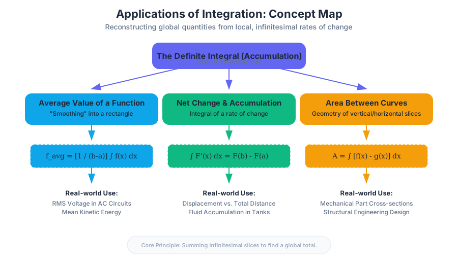
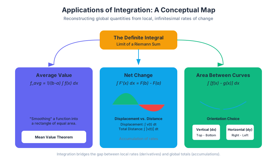
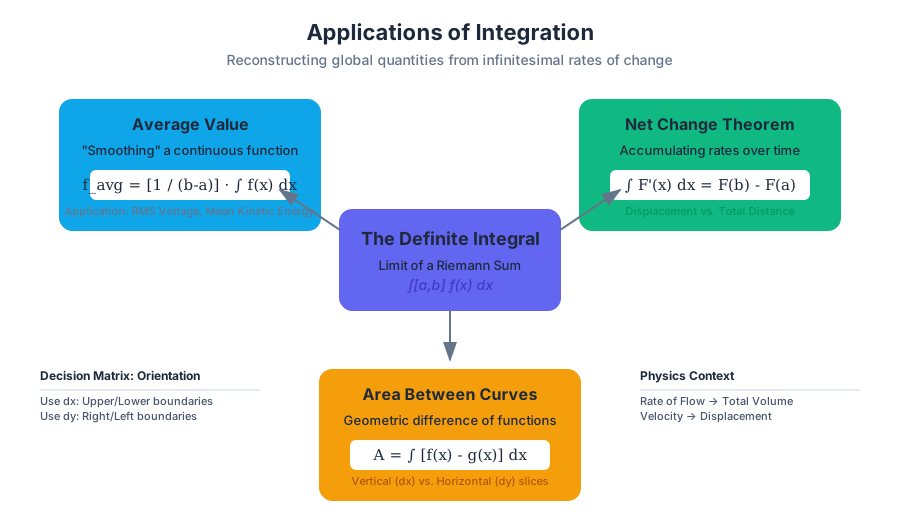
Parametric, Polar, and Vector Functions
Key concepts: Parametric Derivatives · Arc Length · Vector-Valued Functions · Polar Area
Extending calculus to non-Cartesian coordinate systems and planar motion.
Parametric, Polar, and Vector Functions
The transition from single-variable Cartesian calculus to parametric, vector-valued, and polar functions represents a fundamental shift in mathematical modeling. While standard functions of the form $y = f(x)$ are sufficient for describing simple relationships where every input has exactly one output, they fail to capture the complexity of paths that double back on themselves, circular motion, or objects moving through space over time. By decoupling the coordinates and introducing independent parameters or angular perspectives, we gain the ability to describe the physical world—from the trajectory of a SpaceX Falcon 9 to the electromagnetic patterns of a dipole antenna—with surgical precision.
Parametric Equations: Decoupling the Path
A parametric equation defines a group of quantities as explicit functions of one or more independent variables called parameters. In two-dimensional calculus, we typically define $x$ and $y$ as functions of time $t$: $$x = f(t), \quad y = g(t)$$ This allows us to describe curves that are not functions in the Cartesian sense, such as circles, ellipses, and the intricate loops of a cycloid.
Parametric Derivatives
To find the slope of the tangent line to a parametric curve at a specific point, we use the version of the Chain Rule adapted for parameters. Since $y$ is a function of $t$ and $t$ is implicitly a function of $x$, we have: $$\frac{dy}{dx} = \frac{dy/dt}{dx/dt}, \quad \text{provided } \frac{dx}{dt} \neq 0$$
The second derivative is more nuanced and is a frequent source of error for students. It represents the rate of change of the slope with respect to $x$: $$\frac{d^2y}{dx^2} = \frac{\frac{d}{dt}\left(\frac{dy}{dx}\right)}{\frac{dx}{dt}}$$
Key Insight: The second derivative is not simply $y''(t) / x''(t)$. You must differentiate the first derivative with respect to $t$ and then divide by the original "horizontal speed" $dx/dt$.
Arc Length in Parametric Form
The arc length $L$ of a smooth curve defined parametrically from $t=a$ to $t=b$ is derived from the Pythagorean theorem applied to infinitesimal displacements $dx$ and $dy$: $$L = \int_{a}^{b} \sqrt{\left(\frac{dx}{dt}\right)^2 + \left(\frac{dy}{dt}\right)^2} , dt$$
| Feature | Cartesian $y=f(x)$ | Parametric $x(t), y(t)$ |
|---|---|---|
| Slope ($dy/dx$) | $f'(x)$ | $\frac{y'(t)}{x'(t)}$ |
| Arc Length | $\int \sqrt{1 + [f'(x)]^2} dx$ | $\int \sqrt{[x'(t)]^2 + [y'(t)]^2} dt$ |
| Directionality | Left-to-right only | Defined by increasing $t$ |
| Self-Intersection | Impossible | Possible (e.g., figure-eight) |
import numpy as np
from scipy.integrate import quad

def calculate_parametric_arc_length(x_func, y_func, t_start, t_end):
    """
    Calculates the arc length of a parametric curve using numerical integration.

    Args:
        x_func: Function representing dx/dt
        y_func: Function representing dy/dt
        t_start: Lower bound of parameter t
        t_end: Upper bound of parameter t
    """
    # The integrand: sqrt((dx/dt)^2 + (dy/dt)^2)
    integrand = lambda t: np.sqrt(x_func(t)**2 + y_func(t)**2)

    length, error = quad(integrand, t_start, t_end)
    return length

# Example: Arc length of a circle with radius 1 (t from 0 to 2*pi)
# x = cos(t) -> dx/dt = -sin(t)
# y = sin(t) -> dy/dt = cos(t)
circle_len = calculate_parametric_arc_length(lambda t: -np.sin(t), lambda t: np.cos(t), 0, 2*np.pi)
print(f"Circumference: {circle_len:.5f}") # Should be 6.28319
Vector-Valued Functions and Planar Motion
A Vector-Valued Function (VVF) maps a scalar parameter (usually time $t$) to a vector. In 2D, this is denoted as $\mathbf{r}(t) = \langle x(t), y(t) \rangle$ or $\mathbf{r}(t) = x(t)\mathbf{i} + y(t)\mathbf{j}$. VVFs are the standard language for physics and engineering because they elegantly encapsulate both magnitude and direction.
Kinematics: Position, Velocity, and Acceleration
The calculus of vectors is performed component-wise. If $\mathbf{r}(t)$ is the position vector:
- Velocity: $\mathbf{v}(t) = \mathbf{r}'(t) = \langle x'(t), y'(t) \rangle$
- Acceleration: $\mathbf{a}(t) = \mathbf{v}'(t) = \mathbf{r}''(t) = \langle x''(t), y''(t) \rangle$
- Speed: The magnitude of the velocity vector, $|\mathbf{v}(t)| = \sqrt{(x'(t))^2 + (y'(t))^2}$.
- Total Distance: The integral of speed over time: $\int_{a}^{b} |\mathbf{v}(t)| , dt$.
Displacement vs. Distance Traveled
It is vital to distinguish between the vector change in position and the total path length.
- Displacement: $\int_{a}^{b} \mathbf{v}(t) , dt = \mathbf{r}(b) - \mathbf{r}(a)$ (a vector).
- Total Distance: $\int_{a}^{b} |\mathbf{v}(t)| , dt$ (a scalar).
\begin{aligned}
&\text{Derivation of Second Derivative in Parametric Form:} \\
&\text{Let } y' = \frac{dy}{dx} = \frac{g'(t)}{f'(t)} \\
&\frac{d^2y}{dx^2} = \frac{d}{dx} \left( y' \right) \\
&\text{By the Chain Rule: } \frac{d}{dx}(y') = \frac{d/dt(y')}{dx/dt} \\
&\text{Therefore: } \frac{d^2y}{dx^2} = \frac{\frac{d}{dt} \left[ \frac{g'(t)}{f'(t)} \right]}{f'(t)}
\end{aligned}
Polar Coordinates: The Angular Perspective
While Cartesian coordinates use a grid of rectangles, Polar Coordinates describe points based on their distance from the origin ($r$) and their angle from the positive x-axis ($\theta$). This system is indispensable for problems involving central forces or rotational symmetry.
Conversion Identities
To bridge the gap between systems, we use:
- $x = r \cos \theta$
- $y = r \sin \theta$
- $r^2 = x^2 + y^2$
- $\tan \theta = \frac{y}{x}$
Derivatives in Polar Form
When we have a curve $r = f(\theta)$, we often want to find the slope $dy/dx$ in the Cartesian plane. We treat $\theta$ as a parameter and apply the parametric derivative formula: $$\frac{dy}{dx} = \frac{dy/d\theta}{dx/d\theta} = \frac{\frac{d}{d\theta}(r \sin \theta)}{\frac{d}{d\theta}(r \cos \theta)} = \frac{\frac{dr}{d\theta}\sin \theta + r\cos \theta}{\frac{dr}{d\theta}\cos \theta - r\sin \theta}$$
Area Bounded by Polar Curves
The area in polar coordinates is calculated by summing the areas of infinitesimal sectors (triangular "slices"). The area of a sector with radius $r$ and central angle $d\theta$ is $\frac{1}{2}r^2 d\theta$. $$A = \int_{\alpha}^{\beta} \frac{1}{2} [r(\theta)]^2 , d\theta$$
| Curve Type | Equation Form | Visual Characteristic |
|---|---|---|
| Cardioid | $r = a(1 \pm \cos \theta)$ | Heart-shaped, passes through origin |
| Limacon | $r = a \pm b \cos \theta$ | Can have an inner loop if $a < b$ |
| Rose Curve | $r = a \cos(n\theta)$ | $n$ petals if $n$ is odd, $2n$ petals if $n$ is even |
| Circle | $r = a \cos \theta$ | Centered on the x-axis (if cos) or y-axis (if sin) |
// Example: Drawing a Polar Rose in a p5.js-like environment
function drawRose(n, d, amplitude) {
  beginShape();
  // k = n/d is the 'petal density'
  let k = n / d;
  for (let a = 0; a < TWO_PI * d; a += 0.02) {
    let r = amplitude * cos(k * a);
    let x = r * cos(a);
    let y = r * sin(a);
    vertex(x, y);
  }
  endShape(CLOSE);
}

// Usage: drawRose(5, 1, 100) creates a 5-petal rose
// Usage: drawRose(4, 1, 100) creates an 8-petal rose
Advanced Applications and Pitfalls
Area Between Two Polar Curves
When finding the area between two curves $r_{outer}$ and $r_{inner}$, the formula is: $$A = \int_{\alpha}^{\beta} \frac{1}{2} \left( [r_{outer}(\theta)]^2 - [r_{inner}(\theta)]^2 \right) , d\theta$$
Common Pitfall: Students often try to integrate $(r_{outer} - r_{inner})^2$. This is incorrect. You must square the individual radii first, then subtract, reflecting the subtraction of two distinct sector areas.
The "Origin" Problem in Polar Area
When calculating the area of a loop (like in a Limacon), you must find the values of $\theta$ where the curve hits the origin ($r=0$). These values become your limits of integration. Failure to find these precisely often leads to including "ghost" area or missing the inner loop entirely.
Intersection of Polar Curves
Finding the intersection of two polar curves is more complex than Cartesian curves because a single point in space has infinitely many polar representations: $(r, \theta)$, $(-r, \theta + \pi)$, etc.
- Set $r_1(\theta) = r_2(\theta)$ and solve for $\theta$.
- Check if the origin ($r=0$) is a point of intersection for both, even if at different $\theta$ values.
- Graph the functions to identify intersections that occur due to the periodicity of $\theta$.
Summary of Formulae
| Concept | Parametric ($t$) | Polar ($\theta$) |
|---|---|---|
| Coordinate Conversion | N/A | $x=r\cos\theta, y=r\sin\theta$ |
| First Derivative | $\frac{y'(t)}{x'(t)}$ | $\frac{r'\sin\theta + r\cos\theta}{r'\cos\theta - r\sin\theta}$ |
| Arc Length | $\int \sqrt{(x')^2 + (y')^2} dt$ | $\int \sqrt{r^2 + (r')^2} d\theta$ |
| Area | $\int y , dx = \int g(t) f'(t) dt$ | $\int \frac{1}{2} r^2 d\theta$ |
| Horizontal Tangent | $y'(t) = 0$ | $\frac{dy}{d\theta} = 0$ |
| Vertical Tangent | $x'(t) = 0$ | $\frac{dx}{d\theta} = 0$ |
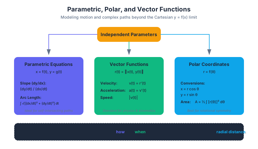
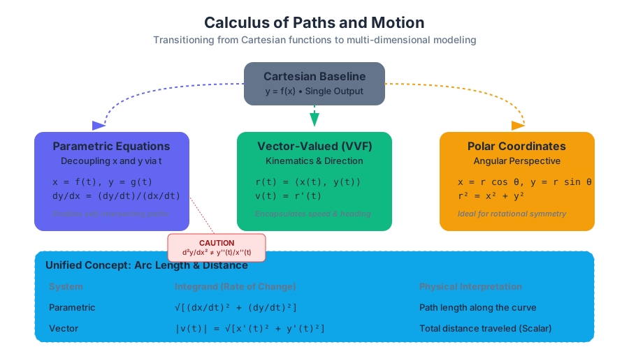
Infinite Sequences and Series
Key concepts: Convergence Tests · Taylor/Maclaurin Series · Power Series · Lagrange Error Bound
Determining convergence and representing functions as power series.
Infinite Sequences and Series
The study of infinite sequences and series represents one of the most profound leaps in mathematical thought. It is the transition from the finite—things we can count and add by hand—to the infinite, where intuition often fails and rigorous logic must take over. In the context of calculus, series allow us to represent transcendental functions (like $e^x$, $\sin(x)$, and $\ln(x)$) as "infinite polynomials." This transformation is not merely a theoretical curiosity; it is the engine that powers modern computing, signal processing, and physics.
Foundations: Sequences vs. Series
Before we can sum an infinite number of terms, we must understand the individual terms themselves. A sequence ${a_n}$ is an ordered list of numbers defined by a function whose domain is the set of positive integers. A series $\sum a_n$ is the sum of the terms of a sequence.
The most critical question we ask of any infinite series is: Does it converge?
Definition: Convergence A series $\sum_{n=1}^{\infty} a_n$ converges to a sum $S$ if the sequence of its partial sums ${S_k}$, where $S_k = \sum_{n=1}^{k} a_n$, approaches a finite limit $S$ as $k \to \infty$. If the limit of partial sums does not exist or is infinite, the series diverges.
The Divergence Test (nth Term Test)
The first "sanity check" for any series is the Divergence Test. If the individual terms $a_n$ do not approach zero as $n$ goes to infinity, the sum cannot possibly settle at a finite value.
- If $\lim_{n \to \infty} a_n \neq 0$, then $\sum a_n$ diverges.
- If $\lim_{n \to \infty} a_n = 0$, the test is inconclusive. (Recall the Harmonic Series $\sum \frac{1}{n}$, which diverges even though its terms go to zero).
Convergence Tests: The Analytical Toolbox
Determining convergence is rarely as simple as looking at the limit of the nth term. We require a suite of tests, each suited to different "shapes" of functions.
Summary of Convergence Tests
| Test Name | Series Form | Condition for Convergence | Condition for Divergence |
|---|---|---|---|
| Geometric Series | $\sum ar^n$ | $\vert r\vert < 1$ | $\vert r\vert \geq 1$ |
| p-Series | $\sum \frac{1}{n^p}$ | $p > 1$ | $p \leq 1$ |
| Integral Test | $\sum f(n)$ | $\int_{1}^{\infty} f(x) dx$ converges | $\int_{1}^{\infty} f(x) dx$ diverges |
| Ratio Test | $\sum a_n$ | $\lim_{n \to \infty} \vert \frac{a_{n+1}}{a_n}\vert < 1$ | $\lim_{n \to \infty} \vert \frac{a_{n+1}}{a_n}\vert > 1$ |
| Comparison Test | $\sum a_n$ | $a_n \leq b_n$ and $\sum b_n$ converges | $a_n \geq b_n$ and $\sum b_n$ diverges |
| Alt. Series Test | $\sum (-1)^n b_n$ | $b_{n+1} \leq b_n$ AND $\lim_{n \to \infty} b_n = 0$ | If limit $\neq 0$, diverges by nth term |
The Ratio Test: The Powerhouse of Power Series
The Ratio Test is perhaps the most vital tool for the calculus student. It measures the "growth rate" of the series terms. If the ratio of a term to its predecessor is less than 1 in the limit, the series behaves like a decaying geometric series and converges.
import numpy as np

def check_ratio_convergence(sequence_func, n_terms=1000):
    """
    Numerically estimates the limit of the ratio |a_{n+1} / a_n|.
    This is a low-level heuristic to visualize the Ratio Test.
    """
    ratios = []
    for n in range(1, n_terms):
        try:
            current_term = abs(sequence_func(n))
            next_term = abs(sequence_func(n + 1))

            if current_term == 0:
                continue

            ratio = next_term / current_term
            ratios.append(ratio)
        except OverflowError:
            return float('inf')

    # Return the last ratio as an approximation of the limit
    return ratios[-1]

# Example: a_n = 3^n / n!
# We expect this to converge because factorials grow faster than exponentials.
example_seq = lambda n: (3**n) / np.math.factorial(n)
limit_approx = check_ratio_convergence(example_seq)

print(f"Approximated Ratio Limit: {limit_approx:.4f}")
print("Status:", "Convergent" if limit_approx < 1 else "Divergent or Inconclusive")
Absolute vs. Conditional Convergence
A series $\sum a_n$ is absolutely convergent if the series of absolute values $\sum |a_n|$ converges. If $\sum a_n$ converges but $\sum |a_n|$ diverges (like the alternating harmonic series $\sum \frac{(-1)^n}{n}$), the series is conditionally convergent. This distinction is crucial because absolutely convergent series can be rearranged in any order without changing the sum—a property not shared by conditionally convergent series.
Power Series and the Interval of Convergence
A Power Series is a series of the form: $$\sum_{n=0}^{\infty} c_n (x - a)^n = c_0 + c_1(x-a) + c_2(x-a)^2 + \dots$$ where $a$ is the center and $c_n$ are coefficients. Unlike constant series, a power series may converge for some values of $x$ and diverge for others.
Radius ($R$) and Interval ($I$) of Convergence
Every power series has a Radius of Convergence $R$.
- If $R=0$, the series converges only at $x=a$.
- If $R=\infty$, the series converges for all real $x$.
- If $0 < R < \infty$, the series converges if $|x-a| < R$ and diverges if $|x-a| > R$.
Crucial Step: To find the Interval of Convergence, you must use the Ratio Test to find $R$, then manually check the endpoints ($x = a-R$ and $x = a+R$) using other convergence tests, as the Ratio Test is inconclusive when the limit equals 1.
| Scenario | Convergence Behavior |
|---|---|
| Inside the Radius | Absolute Convergence |
| Outside the Radius | Divergence |
| At the Endpoints | Varies (Can be Absolute, Conditional, or Divergent) |
Taylor and Maclaurin Series
If we assume a function $f(x)$ can be represented as a power series, we can derive the coefficients by repeatedly differentiating the series and evaluating it at the center.
The Derivation
Suppose $f(x) = \sum_{n=0}^{\infty} c_n (x-a)^n$.
- $f(a) = c_0$
- $f'(x) = c_1 + 2c_2(x-a) + 3c_3(x-a)^2 \dots \implies f'(a) = c_1$
- $f''(x) = 2c_2 + 6c_3(x-a) \dots \implies f''(a) = 2c_2 \implies c_2 = \frac{f''(a)}{2!}$
- Generalizing this, we find the Taylor Coefficient: $c_n = \frac{f^{(n)}(a)}{n!}$
% Mathematical Derivation of the Taylor Series Formula
f(x) = \sum_{n=0}^{\infty} \frac{f^{(n)}(a)}{n!} (x-a)^n

\text{When the center } a = 0, \text{ the series is called a Maclaurin Series:}
f(x) = f(0) + f'(0)x + \frac{f''(0)}{2!}x^2 + \frac{f'''(0)}{3!}x^3 + \dots
Common Maclaurin Series to Memorize
These series are the building blocks for more complex approximations.
| Function | Maclaurin Series | Interval of Convergence |
|---|---|---|
| $\frac{1}{1-x}$ | $\sum_{n=0}^{\infty} x^n = 1 + x + x^2 + \dots$ | $(-1, 1)$ |
| $e^x$ | $\sum_{n=0}^{\infty} \frac{x^n}{n!} = 1 + x + \frac{x^2}{2!} + \dots$ | $(-\infty, \infty)$ |
| $\sin(x)$ | $\sum_{n=0}^{\infty} \frac{(-1)^n x^{2n+1}}{(2n+1)!} = x - \frac{x^3}{3!} + \frac{x^5}{5!} \dots$ | $(-\infty, \infty)$ |
| $\cos(x)$ | $\sum_{n=0}^{\infty} \frac{(-1)^n x^{2n}}{(2n)!} = 1 - \frac{x^2}{2!} + \frac{x^4}{4!} \dots$ | $(-\infty, \infty)$ |
| $\ln(1+x)$ | $\sum_{n=1}^{\infty} \frac{(-1)^{n-1} x^n}{n} = x - \frac{x^2}{2} + \frac{x^3}{3} \dots$ | $(-1, 1]$ |
Error Analysis: How Wrong Are We?
In practice, we cannot sum an infinite number of terms. We use a Taylor Polynomial of degree $n$, denoted $P_n(x)$, to approximate the function. The difference between the actual function and the polynomial is the remainder (or error): $R_n(x) = f(x) - P_n(x)$.
1. Alternating Series Error Bound
If a series satisfies the Alternating Series Test, the error in using the $n$-th partial sum is less than or equal to the magnitude of the first unused term. $$|R_n| \leq |a_{n+1}|$$
2. Lagrange Error Bound
For non-alternating series (or a more general bound), we use the Lagrange Error Bound. It states that for a Taylor polynomial of degree $n$ centered at $a$: $$|R_n(x)| \leq \frac{M}{(n+1)!} |x-a|^{n+1}$$ where $M$ is the maximum value of the $(n+1)$-th derivative $|f^{(n+1)}(z)|$ for all $z$ between $x$ and $a$.
Worked Example: Approximating $\sin(0.1)$
Suppose we use the 3rd-degree Maclaurin polynomial for $\sin(x)$ to estimate $\sin(0.1)$. $P_3(x) = x - \frac{x^3}{3!}$ $P_3(0.1) = 0.1 - \frac{(0.1)^3}{6} = 0.1 - 0.0001666... = 0.0998333...$
To find the Lagrange Error Bound ($n=3$): We need the 4th derivative of $\sin(x)$, which is $\sin(x)$. The maximum value of $|\sin(z)|$ on the interval $[0, 0.1]$ is $\sin(0.1)$, but for simplicity, we often use the global maximum $M=1$. $|R_3(0.1)| \leq \frac{1}{(3+1)!} |0.1 - 0|^{4} = \frac{0.0001}{24} \approx 0.00000416$
This tells us our approximation $0.0998333$ is accurate to at least 5 decimal places.
# Real-world usage: Using a symbolic math library to compute
# Taylor expansions and verify error bounds.

# Install sympy if not present
pip install sympy

# Python script to generate Taylor Series
python3 -c "
from sympy import symbols, series, sin, pi
x = symbols('x')
# Generate 6th order Taylor expansion of sin(x) centered at 0
expr = sin(x)
t_series = expr.series(x, 0, 6)
print(f'Taylor Series of sin(x): {t_series}')

# Evaluate at x=0.1
val = t_series.removeO().subs(x, 0.1)
print(f'Approximate value at 0.1: {val.evalf()}')
"
Common Pitfalls and Misconceptions
- Confusing Sequences and Series: A sequence can converge to zero while its series diverges (e.g., the harmonic series). Always check if you are being asked about the list of numbers or the sum.
- Forgetting the Center: When using the Taylor formula, ensure all derivatives are evaluated at the center $a$, not at $x$.
- Endpoint Neglect: The Ratio Test only gives the open interval. You must test the endpoints separately to determine if the interval is $(, )$, $[, )$, $(, ]$, or $[, ]$.
- The "M" in Lagrange: Students often struggle to find $M$. Remember, $M$ is an upper bound. If you can't find the exact maximum of the $(n+1)$-th derivative, any value that is definitely larger than the maximum (like 1 for sine/cosine) will technically work, though it will give a looser bound.
Summary Table: Error Bounds Comparison
| Feature | Alternating Series Bound | Lagrange Error Bound |
|---|---|---|
| Applicability | Only alternating series with decreasing terms | Any function with $n+1$ derivatives |
| Ease of Use | Very Easy (just look at next term) | Moderate (requires $(n+1)$-th derivative) |
| Precision | Usually tighter for alternating series | General-purpose |
| Formula | $\vert a_{n+1}\vert $ | $\frac{max\vert f^{(n+1)}(z)\vert }{(n+1)!}\vert x-a\vert ^{n+1}$ |
Author Note: This article serves as a deep-dive into the mechanics of infinite series. For further exploration, one might look into Fourier Series, which use trigonometric functions instead of polynomials to represent periodic signals, or Complex Analysis, where the radius of convergence is visualized as a literal disk in the complex plane.
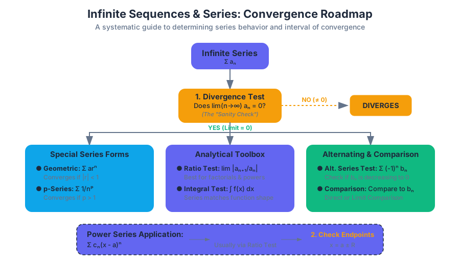
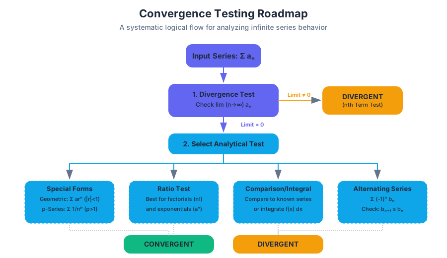
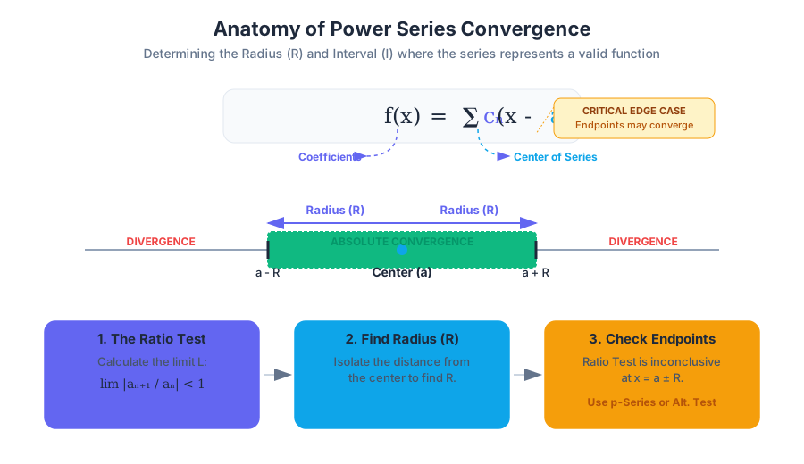
AP Exam Preparation (FRQs)
Key concepts: FRQ Strategies · Scoring Rubrics · Past Exam Analysis
Review of past Free Response Questions to master exam strategies.
AP Exam Preparation (FRQs)
The Free Response Question (FRQ) section of the AP Calculus BC exam represents the ultimate crucible for demonstrating mathematical mastery. Unlike the multiple-choice section, which tests recognition and rapid computation, the FRQs demand a synthesis of conceptual depth, procedural fluency, and—most importantly—mathematical communication. Comprising 50% of the total exam score, the six FRQs are designed to evaluate a student's ability to solve complex, multi-step problems and justify their reasoning using precise notation.
The Anatomy of the FRQ Section
The FRQ section is divided into two distinct parts, structured to test both the student's ability to leverage technology and their fundamental analytical skills.
| Part | Questions | Time | Calculator Usage | Focus |
|---|---|---|---|---|
| Part A | 1 & 2 | 30 Minutes | Required | Modeling, complex integration, data analysis, and intersection of curves. |
| Part B | 3, 4, 5, & 6 | 60 Minutes | Prohibited | Theoretical proofs, slope fields, Taylor series, and fundamental theorems. |
The "Golden Rule" of FRQs: A "bald answer" (an answer with no supporting work) will almost always receive 0 points, even if numerically correct. The AP graders (Readers) are looking for the "setup"—the definite integral, the derivative expression, or the initial equation—that leads to the result.
Scoring Rubrics and the "Art of Justification"
Each FRQ is worth 9 points, regardless of difficulty. These points are distributed based on a specific rubric developed by the College Board. Understanding the rubric is as important as understanding the calculus itself.
Point Distribution Heuristics
Points are typically awarded for:
- The Setup: Writing the correct integral or derivative expression (e.g., $\int_{0}^{5} v(t) dt$).
- The Intermediate Step: Showing the application of a theorem (e.g., identifying that $f'(x)$ changes from positive to negative).
- The Answer: The final numerical value, usually rounded to three decimal places.
- The Justification: A sentence explaining why a conclusion was reached, often citing a specific theorem (MVT, IVT, EVT, or the Second Derivative Test).
Common Justification Requirements
| Scenario | Required Justification Language | Key Theorem/Test |
|---|---|---|
| Relative Extrema | "$f'(x)$ changes from positive to negative at $x=c$." | First Derivative Test |
| Absolute Extrema | "Check candidates (critical points) and endpoints in a table of values." | Extreme Value Theorem (EVT) |
| Existence of a Value | "Since $f(x)$ is continuous and $k$ is between $f(a)$ and $f(b)$..." | Intermediate Value Theorem (IVT) |
| Existence of a Slope | "Since $f(x)$ is differentiable on $(a, b)$ and continuous on $[a, b]$..." | Mean Value Theorem (MVT) |
| Convergence of Series | "The terms are positive, decreasing, and $\lim_{n \to \infty} a_n = 0$." | Alternating Series Test |
Strategic Problem-Solving Archetypes
The AP Calculus BC exam tends to cycle through several "Type" problems. Mastering these archetypes allows students to recognize the required "playbook" as soon as they read the prompt.
1. Rate In / Rate Out (Accumulation)
These problems involve a function $R(t)$ representing the rate at which something enters a system and $E(t)$ representing the rate at which it leaves.
- The Total Amount: $A(t) = A(0) + \int_{0}^{t} (R(s) - E(s)) ds$.
- Optimization: To find the maximum amount, find where $A'(t) = R(t) - E(t) = 0$.
2. Particle Motion (Parametric and Vector-Valued)
In Calculus BC, motion is often two-dimensional.
- Position: $x(t), y(t)$ or $\vec{r}(t) = \langle x(t), y(t) \rangle$.
- Velocity: $\vec{v}(t) = \langle x'(t), y'(t) \rangle$.
- Speed: $|\vec{v}(t)| = \sqrt{(x'(t))^2 + (y'(t))^2}$.
- Total Distance Traveled: $\int_{a}^{b} \sqrt{(x'(t))^2 + (y'(t))^2} dt$.
3. Area and Volume
These problems require finding the area between curves or the volume of a solid of revolution/cross-section.
- Area: $\int_{a}^{b} (\text{top} - \text{bottom}) dx$ or $\int_{c}^{d} (\text{right} - \text{left}) dy$.
- Volume (Washers): $\pi \int_{a}^{b} (R_{outer}^2 - R_{inner}^2) dx$.
- Polar Area: $\frac{1}{2} \int_{\alpha}^{\beta} [r(\theta)]^2 d\theta$.
4. Taylor and Maclaurin Series
The "Question 6" of the BC exam is almost always a power series problem.
- General Form: $P_n(x) = \sum_{n=0}^{\infty} \frac{f^{(n)}(c)}{n!}(x-c)^n$.
- Error Bounds: Using the Alternating Series Error Bound or the Lagrange Error Bound: $E_n(x) \leq \frac{\max|f^{(n+1)}(z)|}{(n+1)!}|x-c|^{n+1}$.
Implementation: Numerical and Algorithmic Perspectives
To truly understand how these calculus concepts function, we can look at how they are implemented computationally. For instance, the Trapezoidal Rule, a frequent FRQ requirement for estimating integrals from a table, is a simple linear interpolation algorithm.
Low-Level Implementation: Trapezoidal Rule (C)
This code demonstrates how a "Reader" expects you to process a data table. If given a set of points $(x, y)$, the area is the sum of the areas of trapezoids formed between each pair of points.
#include <stdio.h>

/**
 * Calculates the definite integral using the Trapezoidal Rule
 * for non-uniform partitions, as often seen in AP FRQ tables.
 *
 * @param x Array of x-coordinates (time, position, etc.)
 * @param y Array of y-coordinates (velocity, rate, etc.)
 * @param n Number of data points
 * @return Estimated area under the curve
 */
double trapezoidal_rule(double x[], double y[], int n) {
    double total_area = 0.0;
    for (int i = 0; i < n - 1; i++) {
        double width = x[i+1] - x[i];
        double average_height = (y[i] + y[i+1]) / 2.0;
        total_area += width * average_height;
    }
    return total_area;
}

int main() {
    // Example from a typical FRQ table
    double time[] = {0.0, 2.0, 5.0, 7.0, 8.0};
    double velocity[] = {0.0, 10.0, 30.0, 25.0, 20.0};
    int n = 5;

    double distance = trapezoidal_rule(time, velocity, n);
    printf("Estimated Total Distance: %.3f units\n", distance);
    return 0;
}
Mathematical Representation: Euler's Method
Euler's Method is the BC-specific numerical approach for approximating solutions to differential equations. It is essentially a sequence of tangent line approximations.
\begin{aligned}
&\text{Given } \frac{dy}{dx} = f(x, y) \text{ and initial point } (x_0, y_0): \\
&x_{n+1} = x_n + \Delta x \\
&y_{n+1} = y_n + f(x_n, y_n) \cdot \Delta x \\
\\
&\text{Algorithm Step-by-Step:} \\
&\text{1. Identify } \Delta x \text{ (step size).} \\
&\text{2. Calculate slope } m = f(x_n, y_n). \\
&\text{3. Update } y \text{ using } \Delta y = m \cdot \Delta x. \\
&\text{4. Repeat for } k \text{ steps.}
\end{aligned}
Real-World Usage: Slope Field Visualization (Python)
In the non-calculator section, you are often asked to sketch a slope field. In a "senior engineer" context, you would use a vector field plot to analyze the stability of a differential equation.
import numpy as np
import matplotlib.pyplot as plt

def plot_slope_field(func, x_range, y_range, density=20):
    """
    Generates a slope field for dy/dx = func(x, y)
    Similar to FRQ 'Sketch the Slope Field' questions.
    """
    x = np.linspace(x_range[0], x_range[1], density)
    y = np.linspace(y_range[0], y_range[1], density)
    X, Y = np.meshgrid(x, y)

    # Calculate dy/dx at each point
    DY = func(X, Y)
    DX = np.ones(DY.shape) # dx is constant for slope visualization

    # Normalize vectors for uniform arrow length
    norm = np.sqrt(DX**2 + DY**2)
    DX /= norm
    DY /= norm

    plt.figure(figsize=(8, 6))
    plt.quiver(X, Y, DX, DY, color='blue', pivot='mid', alpha=0.6)
    plt.title(r"Slope Field for $\frac{dy}{dx}$")
    plt.xlabel("x")
    plt.ylabel("y")
    plt.grid(True)
    plt.show()

# Example: dy/dx = (x * y) / 2
plot_slope_field(lambda x, y: (x * y) / 2, (-3, 3), (-3, 3))
Past Exam Analysis (2008–2017)
Analyzing a decade of exams reveals consistent patterns in how the College Board tests BC-specific topics.
The "BC-Only" FRQ Topics
While AB and BC share about 60-70% of content, the BC exam consistently dedicates at least two full FRQs to:
- Series: Usually involving a Maclaurin series for a transcendental function, finding the interval of convergence, and using the error bound.
- Parametric/Polar/Vector: Often involving a particle moving in the $xy$-plane or the area inside a polar curve like a limaçon or rose curve.
| Year | Question Type | Focus | Difficulty Note |
|---|---|---|---|
| 2008 | Polar Curves | Area of $r = \theta + \sin(2\theta)$ | Required careful integration by parts. |
| 2011 | Taylor Series | $f(x) = \sin(x^2) + \cos(x)$ | Tested manipulation of known series. |
| 2015 | Differential Eq | $\frac{dy}{dx} = (y-1)^2 \cos(\pi x)$ | Separation of variables with a tricky trig integral. |
| 2017 | Parametric | $\langle x'(t), y'(t) \rangle$ | Focus on position at time $t$ using the Fundamental Theorem. |
Common Pitfalls and How to Avoid Them
Even the strongest students lose points on FRQs due to "unforced errors."
- Radian Mode: The AP exam always uses radians. A calculator in degree mode will produce incorrect answers for every trigonometric sub-part.
- Intermediate Rounding: Never round intermediate steps. Store values in your calculator variables ($A, B, C...$) and only round the final answer to three decimal places.
- The $+C$ Oblivion: In differential equation problems (Separation of Variables), forgetting the constant of integration $+C$ immediately caps your score at usually 2 or 3 out of 9 points. You cannot recover from this error.
- Units of Measure: If a question asks for "the rate of change of the temperature," and the temperature is in Celsius and time is in minutes, the units must be $^\circ C/\text{min}$. If the question asks for the "average temperature," the units are just $^\circ C$.
- Equality Abuse: Do not use the equals sign ($=$) to connect unrelated steps. Use arrows ($\to$) or start new lines. If you write $5+5 = 10 + 2 = 12$, you have written a mathematically false statement ($10=12$), and Readers may penalize "linked expressions."
Advanced Technique: The Fundamental Theorem of Calculus (FTC) in FRQs
The most common application of FTC in FRQs is the "Accumulation Function": $$g(x) = \int_{a}^{x} f(t) dt$$ Students are often given a graph of $f(t)$ and asked questions about $g(x)$.
- $g'(x) = f(x)$: The graph of $f$ is the derivative of $g$.
- $g''(x) = f'(x)$: The slope of the graph of $f$ is the second derivative of $g$.
- Critical Points of $g$: Occur where $f(x) = 0$.
- Inflection Points of $g$: Occur where $f(x)$ has a relative maximum or minimum.
Final Checklist for FRQ Success
Before the exam, ensure you can perform these "Big Four" calculator operations fluently:
- Graph a function in an arbitrary window.
- Find the zeros of a function (intersection with the x-axis).
- Calculate the derivative at a specific point (numerical derivative).
- Calculate the definite integral (numerical integration).
Expert Insight: When asked to find the "Average Value" of a function, use $\frac{1}{b-a} \int_{a}^{b} f(x) dx$. When asked for the "Average Rate of Change," use $\frac{f(b)-f(a)}{b-a}$. Confusing these two is one of the most frequent errors on the exam.
- Term: Lagrange Error Bound Definition: A formula used to find the maximum possible error when using a Taylor polynomial to approximate a function.
- Term: Euler's Method Definition: A numerical procedure for solving ordinary differential equations with a given initial value.
- Term: Interval of Convergence Definition: The set of all real numbers $x$ for which a power series converges.
- Term: Separation of Variables Definition: A method for solving differential equations where all terms involving $y$ are moved to one side and all terms involving $x$ to the other.
- Term: Riemann Sum Definition: A certain kind of approximation of an integral by a finite sum, using rectangles or trapezoids.
- Term: Speed (Vector) Definition: The magnitude of the velocity vector: $\sqrt{(x')^2 + (y')^2}$.
-
Scenario: You are given a table of velocity values $v(t)$ at various times $t$. The question asks for the "total distance" traveled from $t=0$ to $t=10$.
- Question: Which mathematical expression should you set up, and what numerical method is most likely required?
- Answer: $\int_{0}^{10} |v(t)| dt$; Trapezoidal or Riemann sum.
-
Scenario: A series $\sum a_n$ is given where $a_n = \frac{(-1)^n}{n}$.
- Question: Does the series converge absolutely, converge conditionally, or diverge? Justify.
- Answer: Converges conditionally. It converges by the Alternating Series Test, but the absolute value version $\sum \frac{1}{n}$ is the divergent harmonic series.
-
Scenario: You need to find the absolute maximum of $f(x)$ on the closed interval $[1, 5]$.
- Question: According to the Extreme Value Theorem, what specific points must you check?
- Answer: The endpoints ($x=1, x=5$) and any critical points where $f'(x)=0$ or is undefined within the interval $(1, 5)$.
-
Scenario: A polar curve is defined by $r = 3 - 2\cos\theta$.
- Question: What is the integral setup for the area of the region enclosed by this curve?
- Answer: $\frac{1}{2} \int_{0}^{2\pi} (3 - 2\cos\theta)^2 d\theta$.
AP Calculus BC FRQ Mastery Guide
1. The 15-Minute Rule You have an average of 15 minutes per question. If you are stuck on a justification, move to the next computational part. Parts (a), (b), and (c) are often independent.
2. Notation Rigor
- Never write $f(x) = \int f(x)$.
- Always include $dx$ or $dt$ in your integrals.
- Use "$\approx$" for approximations and "$=$" for exact setups.
- If you define a function in your work (e.g., "Let $R(t) = \dots$"), you can use the label $R(t)$ thereafter to save time.
3. Calculator Efficiency
- Store the functions given in the prompt into
Y1andY2immediately. - Use the
nDerivandfnInt(or equivalent) functions rather than trying to integrate complex functions by hand in Part A.
4. The "BC" Differentiators
- Integration by Parts: Remember $uv - \int v du$.
- Partial Fractions: Only required for linear non-repeating factors in the AP curriculum.
- Logistic Growth: Know the form $\frac{dP}{dt} = kP(1 - \frac{P}{L})$, where $L$ is the carrying capacity. The maximum growth rate occurs at $P = L/2$.
- Arc Length: $\int_{a}^{b} \sqrt{1 + [f'(x)]^2} dx$.
5. Final Review Strategy
- Review the 2012-2023 scoring guidelines specifically to see how "Justification Points" are awarded.
- Practice "Question 6" (Series) from at least five different years; it is the most predictable yet most failed question on the exam.
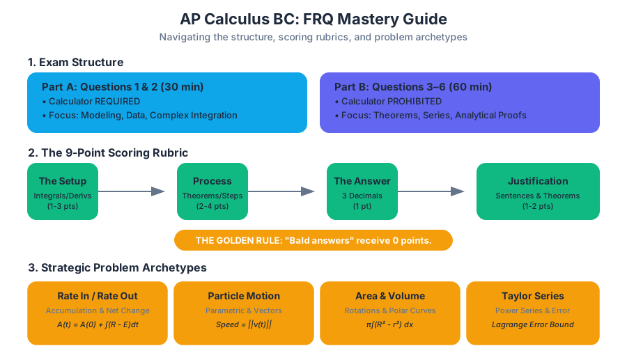
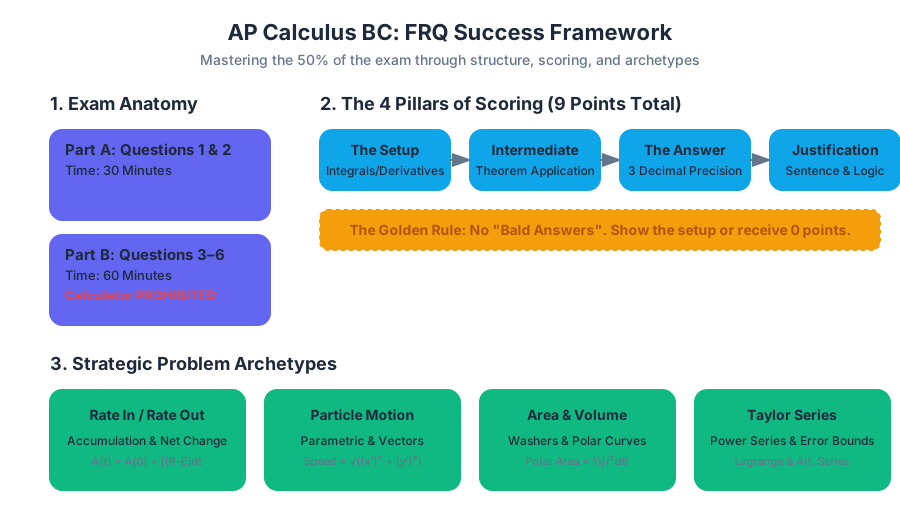
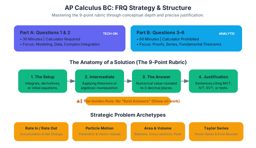
Source Materials
Study AP/College Calculus BC with AI — Free on Lykke
Sign up for free to generate personalized flashcards, quizzes, and study guides from this course. Chat with an AI tutor that knows the material.
Get Started FreeView this course wiki on Lykke · Browse all public course wikis